By applying Itô's lemma and setting g(s) = e−rs − rGs we arrive at the problem sup t∈[0,1] ∫ t. 0 (e−rt − g(s)). 2 ds → min . Example 6 Suppose r > 0 and.
On a class of optimization problems emerging when hedging with short term futures contracts Gunther Leobacher Abstract This paper generalizes earlier work by G. Larcher and the author about hedging with short-term futures contracts, a problem which was considered in connection with the debacle of the German company Metallgesellschaft. While the original problem corresponded to the simplest possible model for the price process, i.e. Brownian motion, we give here solutions to more general models, i.e. a mean reverting model (Ornstein-Uhlenbeck process) and geometric Brownian motion. Furthermore we allow for interest rates greater than 0.
1 Introduction This paper deals with the formulation, partial solution and application of a special class of optimization problems. The simplest such problem, solved in [7], is itself the answer to a question addressed by P. Glasserman in [6]. The question is: Which measurable function g : [0, 1] −→ R minimizes the value of Z t sup (t − g(s))2 ds ? t∈[0,1]
(1)
0
This problem arises when one wants to minimize the maximum “running spot risk” – to be defined later – when one is trying to hedge a long term forward delivery contract with short term futures and when the price process of the commodity in question follows a Brownian motion. In Section 3 we will investigate a more general version of the problem (1), namely: Let φ : [0, 1] −→ R be a decreasing or increasing function and w : [0, 1] −→ R be an a.e. positive, bounded measurable function. Which measurable function g : [0, 1] −→ R minimizes the value of Z t sup (φ(t) − g(s))2 w(s)ds ? (2) t∈[0,1]
0
We will show there that a solution to this general problem always exists and we will further prove properties of the solution which make it possible to find it in special cases. 1
In section 2 we give a brief summary of the origin of the problems (1) and (2) and present more special cases which are of interest in financial applications. The reader who is only interested in the optimization problems may directly jump to section 3. The actual solution of the problems does not make any use of stochastic calculus, or indeed of any financial mathematics.
2 The origin of the problems We consider the following problem discussed in Culp and Miller [3], Mellow and Parsons [8] and by Glasserman [6]: A firm commits to supplying a fixed quantity q of a commodity at a forward price an at dates n = 1, . . . , N . Of course, if the market price of the commodity at time n lies above an , this contract is unfavorable for the firm, since it then sells its product below the market value. On the other hand, if the price decreases, the firm gains due to the contract. To reduce the risk of losses due to the change of the market price the firm might enter into other contracts on the same commodity. A futures contract (long position) is a contract which gives its holder the right and the obligation to buy one piece of the underlying commodity at a certain date at a fixed price. Thus the holder of the future makes gains when there is an increase of the market price and losses in the case of a decrease. It is therefore near at hand to try to use these futures contracts in a hedging strategy. But how exactly should the firm do this? In order to specify and answer this question we formulate a continuous-time version of the contract. Suppose that the price process of the commodity is given by some stochastic differential equation, i.e. dSt = u(t, St )dt + v(t, St )dWt where W is a standard Brownian motion on [0, 1], and u and v are regular enough to guarantee the existence of a solution. We further assume that S0 is deterministic. The firm commits to supplying at each time t in the interval [0, T ] a commodity at the rate q and at the deterministic price at . Of course, there is no loss in assuming T = 1 and q = 1. The discounted, unhedged cumulative cash flow from this contract then is Z t Ct = e−rs (as − Ss ) ds . 0
A short calculation using d(e−rs Ss ) = −re−rs Ss ds + e−rs dSs and St = S0 + gives Z t Z � 1 t −rt e − e−rs dSs . Ct = e−rs (as − S0 )ds + r 0 0 For r = 0 a similar calculation gives Z t Z t Ct = (as − S0 )ds + (s − t) dSs . 0
0
2
Rt 0
dSs (3)
(4)
Alternatively one could let r → 0 in equation (3). Consider now at time t a short term future with maturity t + δ and futures price Ft,t+δ . The discounted (to time 0) payoff of such a contract is e−r(t+δ) (St+δ − Ft,t+δ ) . If we write Ft,t+δ = erδ St + bt,t+δ δ, then we get for the payoff e−r(t+δ) (St+δ − erδ St − bt,t+δ δ) = S˜t+δ − S˜t − e−r(t+δ) bt,t+δ δ , where S˜t = e−rt St is the discounted price-process. bt,t+δ δ is the basis of the future, i.e. the deviation from the “natural” price erδ St , which is the unique arbitrage-free futures price for futures on a commodity with no dividends or cost of carry. The discounted payoff from a hedging strategy holding Gnδ futures at time nδ is therefore k−1 k−1 X X Hkδ := Gnδ (S˜t+δ − S˜t ) − Gnδ e−r(t+δ) bt,t+δ δ n=0
n=0
Letting δ −→ 0 gives
Ht =
Z
0
t
Gs dS˜s −
Z
t
Gs e−rs bs ds , 0
where we assume that bt := limδ→0 bt,t+δ exists and is regular enough to guarantee existence of the integral. Since dS˜t = d(e−rt St ) = −re−rt St dt+e−rt dSt , this means that Z t Z t Ht = e−rs Gs v(s, Ss )dWs + e−rs Gs (u(s, Ss ) − rSs − bs )ds . 0
0
We will maintain the following assumption: Assumption 1 The cash flow H from a hedging strategy G satisfies Z t Ht − E[Ht ] = e−rs Gs v(s, Ss )dWs . 0
Obviously, this assumption is fulfilled if u(s, Ss ) − rSs − bs = 0 a.s. for all s or if Gs (u(s, Ss )−rSs −bs ) is deterministic for almost all s. While u(s, Ss )−rSs −bs = 0 seems to be a very strong requirement it is still reasonable since it is often implied by no-arbitrage arguments. We still allow for the slightly more general case since in the original problem we cannot always assume that the market is completely frictionless. We will see in the examples what particular condition we need to have Assumption 1 satisfied. Now what strategy G should we use? One policy is to demand that the variance of the discounted cumulative hedged cash flow vanishes at the terminal date: V [C1 + H1 ] = 0. 3
It is easy to see that in our examples such a strategy always exists. While such a strategy – called rolling stack – seems appealing it has a disadvantage though: the firm is exposed to a liquidity risk during the hedging period. It has been argued in [3, 6, 8] that it was exactly this exposure which contributed to a large extent to the Metallgesellschaft debacle. So following Glasserman [6] we want to minimize the maximum of the running spot risk instead, i.e. we want to find a strategy G for which sup V (Ct + Ht ) = sup E[(Ct + Ht − E[Ct + Ht ])2 ] → min .
t∈[0,1]
t∈[0,1]
4 2 The maximum running spot risk for the rolling stack strategy in Example 1 is 27 σ = 2 0.148σ . We will see in subsection 3.4 that for some strategy the maximum running spot risk is about 0.0389σ 2. Further discussions about the Metallgesellschaft debacle and related hedging strategies can be found in [1, 2, 4, 5, 10].
Example 1 Let, for example, the price process of our commodity be given by the stochastic differential equation dSt = µdt + σdWt , where µ and σ are constants, σ > 0. Let r = 0. If bs = µ then Assumption 1 holds and we get by equation (4) that Z t (s − t + Gs )dWs . Ct − E[Ct ] + Ht − E[Ht ] = σ 0
By the well-known Itˆo isometry we have Z t Z t 2 2 2 V [Ct + Ht ] = σ E[(s − t + Gs ) ]ds = σ E[(t − s − Gs )2 ]ds . 0
0
From Jensen’s inequality it follows that Z t Z t 2 E[(t − s − Gs ) ]ds ≥ (E[t − s − Gs ])2 ds 0
0
with equality iff Gs is deterministic for almost all s ∈ [0, 1]. So we may w.l.o.g. restrict our search to deterministic strategies. If we write g(s) := s + Gs we arrive at the first problem: find g such that Z t sup (t − g(s))2 ds → min. t∈[0,1]
0
If we relax the requirement bs = µ and only demand that bs be deterministic then we still can observe the following: if we only consider deterministic hedging strategies Gs , then Assumption 1 again holds and we arrive at the same optimization problem. However, in that case there might be a non-deterministic hedging strategy with lower running risk. Finding it seems to be a hopeless task at the present. 4
Example 2 Let r = 0 and let the price process of our commodity be given by the stochastic differential equation dSt = α(ct − St )dt + σdWt , where c is a measurable and bounded real valued function and α is non-negative. This is the model for a price process admitting mean reversion. If the parameter α is positive, then this means that the price of the commodity is permanently drawn towards c. Standard calculations give Z t � � 1 −α(t−s) Ct − E[Ct ] = σ e − 1 dWs 0 α
Using Assumption 1, the deviation of the cumulative hedged cash-flow from its expected value is now given by � Z t� 1 −α(t−s) Ct + Ht − E[Ct + Ht ] = σ (1 − e ) + Gs dWs . α 0 If we set
1 (1 − g(s)eαs ) := Gs α
then Ct + Ht − E[Ct + Ht ] =
σ α
Z
0
t
� e−αt − g(s) eαs dWs .
Therefore we get for the variance Z �2 σ 2 t −αt e − g(s) e2αs ds , 2 α 0
by the Itˆo isometry. If we again want to minimize the running spot risk we see that this problem is again of the general form (2). Here, Assumption 1 will be only fulfilled if bs = α(cs − Ss ). It is easy to see, like in Example 1, that a deterministic strategy is then indeed optimal. Example 3 Another possible way to model the price process is by dSt = σSt dWt . This means that the price process follows a geometric Brownian motion with zero drift. Assuming r = 0 and bs = 0 we have Z t Z t Z t Ct = as ds − tS0 − σ (t − s)Ss dWs and Ht = σ Gs Ss dWs , 0
0
0
such that, if we again assume G to be deterministic and set g(s) = Gs + s, Z t Z t 2 2 2 2 2 V [Ct + Ht ] = σ (t − g(s)) E[Ss ]ds = σ (t − g(s))2 eσ s ds. 0
0
5
So minimizing the supremum of the variances, i.e. the running spot risk, now corresponds to another special case of problem (2). We show that again there is no loss of generality in assuming that G is deterministic: if G is an arbitrary strategy, then E[(t − s − Gs )2 Ss2 ] = E[(t − s − Gs )2
Ss2 ]E[Ss2 ] E[Ss2 ]
= EQ [(t − s − Gs )2 ]E[Ss2 ] ≥ EQ [t − s − Gs ]2 E[Ss2 ] = (t − s − EQ [Gs ])2 E[Ss2 ] , where we have applied Jensen’s inequality with respect to the probability measure Q Ss2 with dQ dP = E[Ss2 ] . Equality holds iff Gs is deterministic Q-a.s.. Observe that, since Ss is positive for all s, Q and P are equivalent measures, such that Gs is also deterministic P-a.s.. As in Example 1 we can relax the requirement bs = 0 to the requirement that bs is deterministic, at the cost that then the optimal deterministic strategy does not necessarily coincide with the overall optimal strategy. Example 4 It would be desirable to consider the more general SDE dSt = µSt dt + σSt dWt , i.e. to allow for non-zero drift. In that case, however, the finite variation part of C, the cumulative unhedged cash-flow, has non-zero variance: Z t (s − t)µ(Ss − E[Ss ])ds Ct + Ht − E[Ct + Ht ] = 0 Z t Z t + (s − t)σSs dWs + Gs Ss dWs 0
0
So here we get a different kind of optimization problem. All we can achieve here with ˜ t := µ t + Wt is a our methods is to change to an equivalent measure for which W σ standard Brownian motion and under which ˜t . dSt = σSt dW So all we can do is to minimize the maximum running spot risk under the new measure. Up to now we have only considered examples where r = 0. The next examples show that for r > 0 we get similar types of problems. Example 5 Let dSt = µdt + σdWt like in Example 1, but now let r > 0. From equations (3) and Assumption 1 it follows that Z � σ t −rt e − e−rs + rGs dWs . Ct − E[Ct ] + Ht − E[Ht ] = r 0 6
By applying Itˆo’s lemma and setting g(s) = e−rs − rGs we arrive at the problem Z t �2 sup e−rt − g(s) ds → min . 0
t∈[0,1]
Example 6 Suppose r > 0 and
dSt = α(ct − St )dt + σdWt . A similar calculation as in Example 2 leads to the problem Z t� �2 e−(α+r)t − g(s) e2αs ds → min . sup t∈[0,1]
0
Example 7 If we consider dSt = σSt dWt with r > 0, we arrive at the problem Z t �2 2 sup e−rt − g(s) eσ s ds → min . t∈[0,1]
0
3 A general optimization problem In this chapter we want to study the following general optimization problem Let φ : [0, 1] −→ R be an increasing or decreasing function and w : [0, 1] −→ R measurable, a.s. positive and bounded. For which measurable function g, if for any, does the functional Z t sup (φ(t) − g(s))2 w(s)ds 0
t∈[0,1]
attain its minimum? We use a similar method as was used in [7] for solving problem (1). However the proofs here are much more involved.
3.1 Preliminary remarks First observe that we may without loss of generality assume that φ is increasing and φ(0) = 0, φ(1) = 1, since for general monotonic φ we may set ˆ := φ(t) − φ(0) . φ(t) φ(1) − φ(0) Then, if we can find gˆ such that sup t∈[0,1]
Z
0
t
ˆ − gˆ(s))2 w(s)ds (φ(t) 7
is minimal, then g(s) := φ(0) + (φ(1) − φ(0))ˆ g (s) , s ∈ [0, 1], solves the original problem. Further we note that, in some way, the case where φ(t) = t ∀t ∈ [0, 1] is already the most general one: suppose φ is continuously differentiable with φ′ (t) 6= 0 ∀t. As mentioned before, it is no restriction to assume that φ is increasing, i.e. φ′ (t) > 0 ∀t and φ(0) = 0, φ(1) = 1. Then we consider Z φ−1 (z) −1 F (φ (z)) = (z − g(s))2 w(s)ds 0 Z z �2 z − g(φ−1 (s)) w(φ−1 (s))(φ−1 )′ (s)ds . = 0
So if we find an optimal gˆ for the problem Z z sup (t − gˆ(s))2 w(s)ds ˆ −→ min , 0
−1
−1 ′
where w(s) ˆ := w(φ (s))(φ ) (s) (note that w ˆ is bounded above and bounded away from 0 if w is) then g(s) = gˆ(φ(s)) is an optimal solution for the original problem. We have chosen to not make much use of this last transformation for two reasons: first, all the results from Subsection 3.2 hold without φ being continuously differentiable. So they are truly more general. Second, the proofs in Subsection (3.3) do not get more involved for more general φ. We will use the simplification in Subsection 3.5, though.
3.2 Existence, Uniqueness and Basic Properties As noted above, we may – and will – assume that φ is increasing. We introduce some notations: for a measurable function h : [0, 1] −→ R we write Z t (φ(t) − h(s))2 w(s)ds , Fh (t) := 0
and we let F := inf supt∈[0,1] Fh (t), where the infimum ranges over all measurable functions h : [0, 1] −→ R. Rt We write W (t) := 0 w(s)ds for t ∈ [0, 1]. Observe that W is strictly increasing. Theorem 1 There exists a non-decreasing function g : [0, 1] −→ R such that F = max Fg (t). t∈[0,1]
Moreover we have φ(s) ≤ g(s) ≤ φ(1) for all s ∈ [0, 1]. Proof: 1. Step: Proof of the inequalities. Any measurable function h which does not fulfill φ(s) ≤ h(s) ≤ φ(1) can be amended: let φ(1) if φ(1) < h(s), h(s) if φ(s) ≤ h(s) ≤ φ(1), h1 (s) := φ(s) if h(s) < φ(s). 8
It is easy to see that h1 improves upon h w.r.t. the optimization problem. 2. Step: Existence of g. If {fi }i≥1 is a sequence of non-decreasing functions fi : [0, 1] −→ [φ(0), φ(1)], then there is a non-decreasing function f : [0, 1] −→ [φ(0), φ(1)] and a sub-sequence {fik }k≥1 such that limk fik = f almost everywhere on [0, 1]. This is an easy consequence of Helly’s selection principle (see for example [9, Kap. VIII, 4, Hilfssatz 2] or [11, Corollary 3.2]). From the bounded convergence theorem it follows that limk fik = f and limk fi2k = f 2 in L1 [0, 1]. Therefore we have Z
lim sup
k→∞ t∈[0,1]
0
and lim sup
k→∞ t∈[0,1]
t
Z
0
(fik (s) − f (s))w(s)ds = 0
t
(fik (s)2 − f (s)2 )w(s)ds = 0 ,
such that limk Ffik = Ff uniformly on [0, 1]. It is therefore enough to show, that for all ε > 0 there exists some non-decreasing h : [0, 1] −→ [φ(0), φ(1)] such that maxt∈[0,1] Fh (t) < F +ε. (With “non-decreasing” being the crucial word, since otherwise this is trivial.) Fix some arbitrary ε > 0 and let ψ : [0, 1] −→ [φ(0), φ(1)] be a step function satisfying maxt∈[0,1] Fψ (t) < F + ε. As in step 1 of the proof we may assume that φ(s) ≤ ψ(s) ≤ φ(1) for all s ∈ [0, 1], since we can find a better function otherwise: If we have to set ψ(s) = φ(s) in some regions, we still can find a step function ψ¯ which ¯ fulfills maxt∈[0,1] Fψ¯ (t) < F + ε and φ(s) ≤ ψ(s) ≤ φ(1). Furthermore we may assume that there are real numbers 0 = t0 < t1 < . . . < tN = 1 and ξ1 , . . . , ξN , such that ξi 6= ξi+1 , 1 ≤ i ≤ N − 1, and ψ(s) = ξi for s ∈ (ti−1 , ti ], 1 ≤ i ≤ N , ψ(0) := φ(0). If ξ1 < ξ2 < . . . < ξN , we are done. Otherwise let 1 ≤ i ≤ N with ξi > ξi+1 . We set ξ :=
(W (ti ) − W (ti−1 ))ξi + (W (ti+1 ) − W (ti ))ξi+1 W (ti+1 ) − W (ti−1 )
and define ψ1 (s) :=
�
ψ(s) ξ
for s ∈ / (ti−1 , ti+1 ], for s ∈ (ti−1 , ti+1 ].
One can check that indeed Fψ1 (t) ≤ Fψ (t) holds for t ∈ [0, 1]. This is done best by considering the intervals [0, ti−1 ], [ti−1 , ti ], [ti , ti+1 ], [ti+1 , 1] separately. We repeat this construction finitely often, ending up with a non-decreasing step function ψk satisfying Fψk (t) < F + ε
∀t ∈ [0, 1].
Thus the result follows. We introduce some extra notation: let g : [0, 1] −→ [φ(0), φ(1)] denote some function that solves our minimization problem, i.e. maxt∈[0,1] Fg (t) = F . Let H be 9
the set where Fg attains its maximum, i.e. H := {t ∈ [0, 1] : Fg (t) = F }. Since Fg is continuous, H is a closed subset of [0, 1]. For a Borel set M ⊆ [0, 1] we write Z µ(M ) := w(s)ds . M
We reveal some basic properties of H and g. Lemma 1 We have 1 ∈ H. Proof: Let us suppose that 1 ∈ / H. Then we have Fg (1) < F . Let t0 := min H and t1 := max H (H is a compact subset of (0, 1)). Fg is a continuous function on [0, 1] with Fg (t1 ) = F and Fg (1) < F . So there exists τ ∈ (t1 , 1) with Fg (1) < Fg (τ ) < Fg (t1 ). For ε > 0 we define Mε := {s ∈ [0, τ ] : g(s) > φ(τ ) + ε}. Observe that Mε is either empty or an interval with right endpoint τ . We show that for a proper choice of ε the latter is the case: an easy calculation gives Z τ 2 Fg (1) − Fg (τ ) ≥ (φ(1) − φ(τ )) W (τ ) + 2(φ(1) − φ(τ )) (φ(τ ) − g(s))w(s)ds . 0
So we have 0
>
Fg (1) − Fg (τ ) 2(φ(1) − φ(τ ))
≥
(φ(1) − φ(τ ))W (τ ) − 2
Z
(g(s) − φ(τ ))w(s)ds −
Mε
≥
Z
(g(s) − φ(τ ))w(s)ds
[0,τ ]\Mε
(φ(1) − φ(τ ))W (τ ) − µ(Mε )(φ(1) − φ(τ ) − ε) − W (τ )ε. 2
Therefore it holds µ(Mε ) ≥
Fg (τ ) − Fg (1) W (τ )(φ(1) − φ(τ ) − 2ε) + , 2(φ(1) − φ(τ ) − ε) 2(φ(1) − φ(τ ))(φ(1) − φ(τ ) − ε)
and we can choose some ε > 0 with µ(Mε ) ≥ W2(τ ) , since the right hand side tends to Fg (τ )−Fg (1) W (τ ) + 2(φ(1)−φ(τ 2 ))2 as ε → 0. In particular Mε is an interval with endpoints η and τ such that µ(Mε ) = W (τ ) − W (η). Now let δ > 0. We define � g(s) − δ s ∈ Mε g1 (s) := g(s) s∈ / Mε . 10
We will show that for appropriate values of δ the function g1 is an enhancement of g. For t ∈ [0, τ ] we have Fg1 (t) =
t
Z
0
(φ(t) − g(s))2 w(s)ds +
−
Z
(φ(t) − g(s) + δ)2 w(s)ds
[0,t]∩Mε
Z
(φ(t) − g(s))2 w(s)ds
[0,t]∩Mε
=
Fg (t) − 2δ
(g(s) − φ(t))w(s)ds + δ 2
Z
Fg (t) − 2δ
(φ(τ ) + ε − φ(t))w(s)ds + δ 2
[0,t]∩Mε
≤
w(s)ds
(5)
[0,t]∩Mε
[0,t]∩Mε
≤
Z
Z
Z
w(s)ds
[0,t]∩Mε 2
Fg (t) − µ([0, t] ∩ Mε )(2δε − δ ).
Here, for sufficient small δ the term 2δε − δ 2 is positive. Furthermore we have W2(τ ) ≤ µ(Mε ) = W (τ ) − W (η) such that W (η) ≤ W2(τ ) . For W −1 ( W2(τ ) ) < t ≤ τ we therefore have µ([0, t] ∩ Mε ) = W (t) − W (η) >
W (τ ) − W (η) ≥ 0 . 2
Now we have Fg1 (t) ≤ Fg (t) for all t ∈ [0, τ ], and
Fg1 (t) < Fg (t) for all t ∈ (W −1 ( W2(τ ) ), τ ].
Now let t ∈ [τ, 1]. Then from equation (5) we have Fg1 (t) ≤ Fg (t) + 2δ(φ(1) − φ(0))µ(Mε ) + δ 2 µ(Mε ). Since Fg (.) is strictly less than F on the compact subset [τ, 1] we can choose δ > 0 such that Fg1 (t) ≤ Fg (t) + 2δ(φ(0) − φ(1))µ(Mε ) + δ 2 µ(Mε ) < F
for all t ∈ [τ, 1].
So we have found a function, g1 , on [0, 1], for which Fg1 ≤ F on [0, 1] and Fg1 < F on [W −1 ( W2(1) ), 1] ⊆ (W −1 ( W2(τ ) ), 1] holds. If we now define H1 := {t ∈ [0, 1] : Fg1 (t) = F }, we have either H1 = ∅ or H1 ⊆ [t0 , W −1 ( W2(1) )). In the first case we have Fg1 < Fg on [0, 1]. In the second case we put t2 := max H1 and apply the same method as above. But this time we can choose τ < W −1 ( W2(1) ) such that we find a function g2 , for which Fg2 ≤ F on [0, 1] and Fg2 < F on [W −1 ( W4(1) ), 1] ⊆ (W −1 ( W2(τ ) ), 1], such that for H2 := {t ∈ [0, 1] : Fg2 (t) = F } we have either H2 = ∅ or H2 ⊆ [t0 , W −1 ( W4(1) )). 11
By repeating this construction we can, after finitely many steps, find a function gk , for which Fgk < F on [0, 1] holds. But this contradicts the optimality of g, and we have 1 ∈ H. Theorem 2 The function g which satisfies F = maxt∈[0,1] Fg (t) is unique (up to a set of measure 0). Proof: Let g1 be another measurable function with max Fg1 (t) = F .
t∈[0,1]
For t ∈ [0, 1] we have F 21 g1 + 12 g (t)
�2 1 1 = (φ(t) − g1 (s)) + (φ(t) − g(s)) w(s)ds 2 2 0 � Z t� 1 1 2 2 (φ(t) − g1 (s)) + (φ(t) − g(s)) w(s)ds ≤ 2 2 0 1 1 = Fg (t) + Fg (t) ≤ F , 2 1 2 Z t�
with equality if and only if g1 (s) = g(s) for a.e. s ∈ [0, t]. Since F 12 g1 + 21 g (t) ≤ F for all t ∈ [0, 1] we have F 12 g1 + 21 g (1) = F by Lemma 1, and therefore equality holds in the above inequality for t = 1. But as we have just noted, this means that g1 equals g a.e.
Lemma 2 H contains at least 2 elements. Proof: Regarding Lemma 1 it is enough to prove H 6= {1}. Suppose instead H = {1}. For ε > 0 put Mε := {s ∈ [0, 1 − 2ε ] : g(s) < φ(1) − ε}. Like in Lemma 1 one can show that µ(Mε ) > 0. Then we can define a function g1 by � g(s) + δ s ∈ Mε g1 (s) := g(s) s∈ / Mε . The function g1 satisfies Fg1 (t) < Fg (t) for all t ∈ [0, 1], contradicting the optimality of g.
Lemma 3 g is constant on the connected components of [0, 1]\H. By “constant” we mean constant almost everywhere, i.e. a measurable function f on a set A is constant if there is some number y such that f (x) = y for a.e. x ∈ A. Observe that, for arbitrary δ > 0, a measurable function f on an interval [a, b] is constant iff f is constant on every sub-interval [τ, η] with length less than δ.
12
Proof of Lemma 3: Suppose on the contrary that g is not constant on one of the connected components of [0, 1]\H. Then there exists some compact sub-interval [a, b] ⊂ [0, 1]\H, such that g is not constant on [a, b]. Observe that supt∈[a,b] Fg (t) < F , since Fg is continuous. For a ≤ τ ≤ η ≤ b let Rη � 1 for s ∈ [τ, η] , W (η)−W (τ ) τ g(σ)w(σ)dσ gτ,η (s) := g(s) for s ∈ / [τ, η] . Then the function [a, b] × [a, b] −→ R � supt∈[τ,η] Fgτ,η (t) (τ, η) 7−→ Fg (τ )
for τ < η , for τ ≥ η
is continuous on [a, b] × [a, b] and has value strictly less than F on the diagonal. Hence there exists δ > 0 such that 0 < η − τ < δ =⇒ sup Fgτ,η (t) < F . t∈[τ,η]
Since g is not constant on [a, b] there exists some interval [τ, η] ⊆ [a, b] such that 0 < η − τ < δ and g is not constant on [τ, η]. Let g1 := gτ,η . Then for t ∈ [0, τ ] we have Fg1 (t) ≤ F . For t ≥ η we have Z t (φ(t) − g1 (s))2 w(s)ds Fg1 (t) = 0 Z τ (φ(t) − g(s))2 w(s)ds = 0
+
η
Z
τ
+
� φ(t) −
Z
t
η
� φ(t) −
η
1 W (η) − W (τ )
(φ(t) − g(s))2 w(s)ds
0 .
Here we have used the fact that g(s) cannot be identically equal to φ(1), since then Fg (1) would be zero, contradicting Lemma 1. Since F ′ is continuous, we have t1 = sup{t ∈ H : t < 1} < 1. Therefore g is constant on [t1 , 1] and, since g(1) = φ(1), g(s) = φ(1) for all s ∈ [t1 , 1]. We have Z t1 (φ(1) − g(s))2 w(s)ds Fg (t1 ) = Fg (1) = 0 Z t1 2 (φ(t1 ) − g(s))w(s)ds + Fg (t1 ), = (φ(1) − φ(t1 )) W (t1 ) + 2(φ(1) − φ(t1 )) 0
15
and therefore 0 6= (φ(1) − φ(t1 ))W (t1 ) = −2 hand
R t1 0
(φ(t1 ) − g(s))w(s)ds. On the other
0 = (Fg )′ (t1 ) = (φ(t1 ) − g(t1 ))2 w(t1 ) + 2φ′ (t1 )
Z
t1 0
(φ(t1 ) − g(s))w(s)ds
such that (φ(t1 ) − g(t1 ))2 w(t1 ) − φ′ (t1 )(φ(1) − φ(t1 ))W (t1 ) = 0 . Since g(t1 ) = φ(1) and (φ(1) − φ(t1 )) 6= 0 this gives the formula. Lemma 7 If I is an open interval contained in H, φ is twice continuously differentiable with φ′ > 0 and w is continuously differentiable and positive on I then g obeys the following ordinary differential equation on I: g ′ (t)
(φ(t) − g(t))w′ (t) 2w(t) ′ 2 (φ(t) − g(t))φ′′ (t) (φ (t)) W (t) − . + (φ(t) − g(t))w(t) 2φ′ (t)
= 2φ′ (t) +
(6)
Proof: Observe that Fg (t) = F for all t ∈ I, such that Fg′ and Fg′′ both vanish on I. Thus we get, by Lemma 4 and Proposition 1 Z t 0 = Fg′ (t) = (φ(t) − g(t))2 w(t) + 2φ′ (t) (φ(t) − g(s))w(s)ds 0
for all t ∈ I. Further we have 0 = Fg′′ (t)
= 2(φ(t) − g(t))(φ′ (t) − g ′ (t))w(t) + (φ(t) − g(t))2 w′ (t) + Z t +2φ′′ (t) (φ(t) − g(s))w(s)ds 0
+2φ′ (t)2 W (t) + 2φ′ (t)(φ(t) − g(t))w(t)
for all t ∈ I. Eliminating the term involving the integral from these two equations and rearranging gives the ODE.
Remark 1 Obviously the ordinary differential equation (6) is of the form g ′ (t) = f (t, g(t)) , where f : Rε −→ R is continuous and satisfies a Lipschitz-condition in the second variable, Rε = {(x, y) : 0 ≤ x ≤ t1 , φ(x) + ε ≤ y ≤ φ(1) + ε} , where 0 < ε is arbitrary. So from Picard’s Theorem it follows that there is a unique solution to the ODE in Rε . 16
3.4 Applications Using the tools we built up to this point it is quite easy to solve the problems emerging in Examples 1 and 2, as well as 3 for a range of choices for σ. The solution to the first one is particularly beautiful, since it can be given analytically. Example 8 Let φ(t) := t, t ∈ function g is given by 3t0 √ σ e− 2 cos( 3σ ) 2 g(s) = 1 −
[0, 1] and w(s) := 1, s ∈ [0, 1]. Then the optimal for s ∈ [0, t0 ],
� �√ √ √ σ for s = − 61 e− 2 3 sin( 23σ ) − 3 cos( 23σ ) π ], with σ ∈ [0, 3√ 3 for s ∈ [1/2, 1],
π √
−
π √
6 3 2 3 where t0 = e 2√3 . Furthermore we have F = e 6√3 = 0.0388532 . . .
Proof: We know that a solution must exist from Theorem 1. First we show that Fg is constant on the interval [t0 , t1 ]. Suppose this were not the case. Then [t0 , t1 ] contains a connected component of the complement of H, i.e. some open interval (τ1 , τ2 ) with τ1 , τ2 ∈ H and (τ1 , τ2 ) ⊆ [0, 1]\H. From Lemma 3 we know that g is constant on (τ1 , τ2 ), so Fg equals some polynomial p on [τ1 , τ2 ], where p has degree 3. p satisfies p(τ1 ) = p(τ2 ) = F and p′ (τ1 ) = p′ (τ2 ) = 0 and is therefore constant. But this contradicts our assumption. From Lemma 5 we know that there exists t0 such that g(t0 ) = φ(t0 ) + 2φ′ (t0 )
W (t0 ) = 3t0 . w(t0 )
From Lemma 6 it follows that t1 is a solution to φ(x) + φ′ (x) i.e.
W (x) = w(x) x+x =
φ(1) , 1,
hence g has the constant value 1 on the interval [ 21 , 1]. Now we investigate the function g on the interval [t0 , 12 ]: Since Fg is constant on this interval we have � � Z t d (t − g(t))2 + 2 (t − g(s))ds 0 = (Fg )′′ (t) = dt 0 = 2(t − g(t))(1 − g ′ (t)) + 4t − 2g(t). This yields the following ordinary differential equation dg 3t − 2g = , dt t−g 17
which we write as
dg dσ dt dσ
3t − 2g t−g
=
for the independent parameter σ. From Lemma 6 we get the initial condition g(t = 1/2) = 1, so we end up with the following initial value problem: dg dσ dt dσ
= 3t − 2g, g(σ = 0) = = t−g
,
t(σ = 0) =
The solution to this system is √ σ 1 σ 3σ g(σ) = e− 2 cos( ) , t(σ) = − e− 2 2 6
1 1 2
! √ √ √ 3σ 3σ 3 sin( ) − 3 cos( ) . 2 2
Finally we have to calculate the value of t0 . We know that g(t = t0 ) = 3t0 . Therefore we look for some σ0 which satisfies g(σ0 ) = 3t(σ0 ). Substituting the above formulas for g and t and simplifying the result gives σ0 = π − 2√ 3
π √ . 3 3
Furthermore we get F = 4t30 = e 6√3 . Example 9 Let φ(t) := e−αt , t ∈ [0, 1] and w(s) := e2αt , s ∈ [0, 1]. Then the optimal function g is of the form −3αt 0 for s ∈ [0, t0 ], e solution of an ODE for s ∈ [t0 , t1 ], g(s) = −α e for s ∈ [t1 , 1], for certain 0 < t0 < t1 < 1.
Proof: We show that Fg is constant on [t0 , t1 ]: Suppose this were not the case. Then [t0 , t1 ] contains a connected component of the complement of H, i.e. some open interval (τ1 , τ2 ) with τ1 , τ2 ∈ H and (τ1 , τ2 ) ⊆ [0, 1]\H. From Lemma 3 we know that g is constant on (τ1 , τ2 ). Therefore we have 3 X Fg (t) = eαt ak e−kαt k=0
for all t ∈ [τ1 , τ2 ] for certain scalars a0 , . . . , a3 . One checks that a0 = a2 = a3 = 0 by using Fg (τ1 ) = Fg (τ2 ) = F and Fg′ (τ1 ) = Fg′ (τ2 ) = 0. Lemma 5 gives g(t0 ) = e−3αt0 , whereas Lemma 6 gives e−αt1 − αe−αt1
e2αt1 − 1 = e−α , 2αe2αt1
18
which one can solve exactly for t1 . The corresponding ODE from Lemma 7 simplifies to � � 2αt α −1 ′ −4αt e −αt g (t) = e −e − 3g(t) . 2 e−αt − g(t) It does not seem very likely that one can solve this ODE exactly. Still it can be solved with standard numerical methods. Also the value of t0 has to be computed numerically.
The function g is for several values of α is shown in figure 3.4. Note that α = 0 coincides with Example 8. g 0.038
α→0
0.030 0.024
α= α=
0.016
α=1
1 4 1 2
0 0
1 t
Figure 1: The optimal g for Example 2 resp. 9. √ 2 Example 10 Let φ(t) := t, t ∈ [0, 1] and w(s) := eσ t , s ∈ [0, 1], where σ 2 < 3− 3. Then the optimal function g is of the form 2 −σ2 t0 ) for s ∈ [0, t0 ], t0 + σ2 (1 − e solution of an ODE for s ∈ [t0 , t1 ], g(s) = σ2 e for s ∈ [t1 , 1],
for certain 0 < t0 < t1 < 1.
Proof: We proceed as before. First we show that Fg is constant on [t0 , t1 ]: suppose instead that there are numbers τ1 , τ2 ∈ [t0 , t1 ] such that Fg (τ1 ) = Fg (τ2 ) = F and Fg (t) < t for all t ∈ (τ1 , τ2 ). From Lemma 3 we know that g is constant on [τ1 , τ2 ], such that for t ∈ (τ1 , τ2 ) we have Z τ1 2 2 eσ τ1 − 1 (τ1 − g(s))2 eσ s ds Fg (t) = (t − τ1 )2 + 2(t − τ ) 1 σ2 0 Z t Z τ1 2 2 σ2 s (t − g(τ1 ))2 eσ s ds (τ1 − g(s)) e ds + + 0
τ1
19
Then, after simplifying, we have for the third derivative � 2 d3 Fg (t) = 6 + 6 σ 2 (t − g(τ1 )) + σ 4 (t − g(τ1 ))2 eσ t , 3 dt √ which is certainly positive for σ 2 < 3 − 3, since |t − g(τ1 )| ≤ 1. Thus Fg′ is strictly concave and can therefore have at most two roots in [τ1 , τ2 ]. Since τ1 and τ2 are maxima of Fg , they have to coincide with the two roots of Fg′ . Now since Fg (t) < F on (τ1 , τ2 ), there has to be a minimum τ3 of Fg on this interval, such that Fg (τ3 ) = 0, but this cannot happen. Therefore the assumption that Fg is not constant on [t0 , t1 ] leads to a contradiction. It remains to compute t1 using Lemma 6, to (numerically) solve the ODE and to find the value of t0 using Lemma 5.
3.5 Towards a solution of the general problem Definition 1 We say the problem sup t∈[0,1]
Z
0
t
(φ(t) − g(s))2 w(s)ds −→ min
is of type m, if (0, 1)\H is the disjoint union of exactly m − 2 open intervals. Note that every problem is at least of type 0, which is the case iff H = [t0 , t1 ] ∪ {1} such that (0, 1)\H = (0, t0 ) ∪ (t1 , 1). Since (0, 1)\H is an open subset of R, it is the disjoint union of at most countably many open intervals. We have seen that the main effort when solving a problem of the form (2) went into showing that H = [t0 , t1 ] ∪ {1}, i.e. into showing that it is of type 0. Note that, even if we find some g1 such that Hg1 := {t ∈ [0, 1] : Fg1 (t) = max Fg1 } = [t0 , t1 ] ∪ {1} , this g1 need not be optimal. Then again, it might happen that such a g1 does not even exist, i.e. that the solution g1 of the ODE (6) starting in (t1 , 1) does not fulfill g1 (t0 ) = φ(t0 ) + 2φ′ (t0 )
W (t0 ) w(t0 )
for any t0 ∈ [0, t1 ]. Since Lemma 5 asserts that for the optimal solution g there is a t0 with W (t0 ) g(t0 ) = φ(t0 ) + 2φ′ (t0 ) w(t0 ) we can conclude that in this case the problem cannot possibly be of type 0.
20
Still, the question as to whether one of these situations may occur or not is completely open. But we can provide a sufficient condition for the function g1 being optimal. We will discuss it only for the case where φ(t) = t (cf. subsection 3.1). Theorem 3 Let w : [0, 1] −→ [0, 1] be a positive, continuously differentiable function. Assume: 1. The equation t+
W (t) = 1, w(t)
has a unique solution t1 ∈ (0, 1). Let f be a solution to the ODE (6) with initial condition f (t1 ) = 1 on (a, t1 ], a minimal. Assume: (t0 ) 2. There exists a unique t0 ∈ [a, t1 ] such that f (t0 ) = t0 + 2 W w(t0 ) .
Set
For τ2 ∈ [t0 , t1 ] define Jτ2 (t)
f (t0 ) s ∈ [0, t0 ] g(s) := f (s) s ∈ [t0 , t1 ] 1 s ∈ [t1 , 1]
:= W (τ2 )(τ2 − t)2 − (t − g(τ2 ))2 (W (τ2 ) − W (t) +(τ2 − g(τ2 )2 w(τ2 )(τ2 − t) ,
(7)
for t ∈ (0, τ2 ]. Assume: 3. For each τ2 ∈ [t0 , t1 ] there is no τ1 such that Jτ2 (τ1 ) = Jτ′ 2 (τ1 ) = 0. If conditions 1, 2 and 3 hold true, then the problem is of type 0 and g is an optimal solution. Proof: Suppose g where not the optimal solution. Let h denote the optimal solution. Then we must have h(s) = 1 = g(s) for all s ∈ [t1 , 1] by Lemma 6. Then h must follow the ODE for at least a little piece. (t1 cannot be an isolated point of H, since (t) then there were another point t < t1 with t + W w(t) = 1, contradicting condition 1.) But at some point τ2 < t1 , h must deviate from g. This can only happen if there is another point τ1 < τ2 such that Fh (τ1 ) = Fh (τ2 ) and Fh′ (τ1 ) = Fh′ (τ2 ) = 0 and such that h is constant on [τ1 , τ2 ]. Then for t ∈ [τ1 , τ2 ] we have Z τ2 Z τ2 2 (t − h(s))2 w(s)ds (8) (t − h(s)) w(s)ds − Fh (t) = t 0 Z τ2 w(s)ds , = t2 A − 2tB + C + (t − h(τ2 ))2 t
21
Rτ Rτ Rτ where A := 0 2 w(s)ds, B := 0 2 h(s)w(s)ds and C := 0 2 h(s)2 w(s)ds. A bit of algebra shows that Z τ2 w(s)ds Jτ2 (t) = t2 A − 2tB + C + (t − h(τ2 ))2 t
−Fh (τ2 ) − Fh′ (τ2 )(t − τ2 )
for t ∈ [0, τ2 ]. From the definition of J and the corresponding properties for Fh we see that J(τ1 ) = J(τ2 ) = 0 and J ′ (τ1 ) = J ′ (τ2 ) = 0. But that contradicts condition 3. The advantage of expression (7) over Equation (8) is that it does not contain any data on h for arguments in [0, τ1 ]. So, if we only know h(τ2 ), as indeed we do since h(τ2 ) = g(τ2 ), then we can actually compute J. And we can find the roots of J and look, whether they are roots of J ′ as well.
4 Remarks and open problems 1. One open question already mentioned above is, whether there exist φ and w such that the corresponding problem is not of type 0. 2. In principle the function Jτ2 from Theorem 3 could also be used to find solutions to problems of higher type. The algorithm will roughly work like this: solve the corresponding ODE, find a τ1 which is root of order 2 for some τ2 , proceed with solving the ODE and so on. However, there is no guaranty that the pair (τ1 , τ2 ) is unique and that the algorithm stops after finitely many steps. So a closer study of the function Jτ2 would be necessary. 3. We have proved the existence and uniqueness of the solution of the problem Let φ : [0, 1] −→ R be a decreasing or increasing function and w : [0, 1] −→ R be an a.e. positive, bounded measurable function. Which measurable function g : [0, 1] −→ R minimizes the value of sup t∈[0,1]
Z
t 0
(φ(t) − g(s))2 w(s)ds ?
(9)
We want to discuss the assumptions on φ and w. Clearly, w is a density function of a measure equivalent to Lebesgue measure if it is bounded and a.e. positive. If we would instead require that w should only be non-negative, then possibly the uniqueness of the solution could fail to hold. Suppose that λ({s : w(s) = 0}) > 0, where λ denotes Lebesgue measure. If g is an optimal solution, then we arrive again at an optimal solution if we alter g on {s : w(s) = 0} in an arbitrary way. It is near at hand that the assumption that φ is strictly monotonic is too strong for the mere existence of solutions. Yet it is possible to provide examples where, for non-monotonic φ, there exists an infinite number of optimal solutions. 22
4. This leads to the following question: Let φ : [0, 1] −→ R be a measurable function and w : [0, 1] −→ R be an a.e. positive, bounded measurable function. Under what conditions on φ does there exist a measurable function g : [0, 1] −→ R which minimizes the value of Z t
sup
t∈[0,1]
0
(φ(t) − g(s))2 w(s)ds ?
References [1] M. J. Brennan and N. I. Crew. Hedging long-maturity commodity commitments with short-dated futures contracts. In A. A. H. Dempster and S. R. Pliska, editors, Mathematics of Derivative Securities, pages 165–189. Cambridge University Press, 1997. [2] W. B¨uhler, O. Korn, and R. Sch¨obel. Hedging long-term forwards with short-term futures: a two-regime approach. Rev. Deriv. Res., 7(3):185–212, 2004. [3] C. L. Culp and M. H. Miller. Metallgesellschaft and the economics of synthetic storage. J. Applied Corporate Finance, 7:62–76, 1995. [4] C. L. Culp and M. H. Miller, editors. Corporate Hedging in Theory and Practice: Lessons from Metallgesellschaft. Risk Books, 1999. [5] F. R. Edwards and M. S. Canter. The collapse of metallgesellschaft: Unhedgeable risks, poor hedging strategy, or just bad luck? The Journal of Futures Markets, 15:211–264, 1995. [6] P. Glasserman. Shortfall risk in long-term hedging with short-term futures contracts. Jouini, E. (ed.) et al., Option pricing, interest rates and risk management. Cambridge: Cambridge University Press. Handbooks in Mathematical Finance. 477-508 (2001)., 2001. [7] G. Larcher and G. Leobacher. An optimal strategy for hedging with short-term futures contracts. Math. Finance, 13(2):331–344, 2003. [8] A. S. Mello and J. E. Parsons. Funding risk and hedge valuation. Working paper, University of Wisconsin, 1995. [9] I.P. Natanson. Theorie der Funktionen einer reellen Ver¨anderlichen. (Mathematische Lehrb¨ucher und Monographien. Bd. VI). Berlin: Akademie- Verlag. XII, 590 S. mit 9 Abb. , 1961. [10] A. Neuberger. Hedging long-term exposures with multiple short-term futures contracts. The Review of Financial Studies, 12(3):429–459, 1999. [11] K. Schrader. A generalization of the Helly selection theorem. Bull. Am. Math. Soc., 78(3):415–419, 1972.
23