On Application of Data Mining in Functional Debug - UCSB ...

On Application of Data Mining in Functional Debug 1

Kuo-Kai Hsieh1 , Wen Chen2 , Li-C Wang1 , Jayanta Bhadra2 Department of Electrical and Computer Engineering, University of California, Santa Barbara 2 Technology Solution Organization,Freescale Semiconductor Inc.

Abstract—This paper investigates how data mining can be applied in functional debug, which is formulated as the problem of explaining a functional simulation error based on humanunderstandable machine states. We present a rule discovery methodology comprising two steps. The first step selects relevant state variables for constructing the mining dataset. The second step applies rule learning to extract rules that differentiates the tests that excite error behavior from those that do not. We explain the dependency of the second step on the first step and considerations for implementing the methodology in practice. Application of the proposed methodology is illustrated through experiments conducted on a recent commercial SoC design.

I. I NTRODUCTION Functional verification relies heavily on simulation. Functional verification starts with a verification plan, specifying the aspects of the design to verify [1]. In constrained random verification, tests are generated by constrained random test generation, which is guided by constraints and biases specified in a test bench (or test template). Verification quality is measured by coverage metrics and coverage results are analyzed to guide the setting of those constraints and biases. In a design process, the design evolves over time. This means that functional verification also evolves accordingly. From one design version to another, functional verification has two important goals: to identify bugs in the current version of the design, and to develop a collection of test benches and specific tests that eventually will be used to simulate the final version of the design. Typically tests that excite design bugs are included in such a collection. In this work, we call a constrained random test generator a randomizer. We call a particular setting of constraints and biases a test bench and a collection of test benches a test plan. A randomizer processes a test bench and produces a set of tests. For example, a test for verifying a processor core is a sequence of assembly instructions. A test for verifying a platform is a sequence of transactions. For test plan development, it often relies on coverage metrics to drive the improvement of a test plan. A popular coverage metric is based on coverage groups where each group consists of coverage points. A coverage point is usually defined as a particular combination of signal values. Suppose a randomizer generates a set of tests for simulation. Suppose some of the tests fail the simulation and others This work is supported in part by Semiconductor Research Corporation 2012-TJ-2268

pass. This is a typical scenario where a verification engineer analyzes the simulation result and tries to locate the source of simulation error. The source can be improper setup of the simulation run, an erroneous checker, or a design bug. In this work, functional debug starts with the two sets of tests and their simulation results. The objective is to discover a rule to explain the difference between these two sets of tests. This is different from traditional view of functional debug where it is the process of starting with failing simulation run and tracing back to the error source. For the reason that will be explained later, it is difficult to apply data mining in the context of locating the error source. Therefore, we formulate the problem differently to enable the application of data mining. In light of our problem formulation, the authors in [2] proposed a data mining methodology that analyzes the simulation traces and the tests to assist in understanding why some tests hit the coverage points and others do not. The result is then used to develop additional constraints for better controllability to hit the points in the coverage group. The work in [2] assumes all required information is contained in the dataset for rule learning. In practice, this is not a realistic assumption. In a particular rule learning run, it is likely that the set of state variables used to encode the simulation data is incomplete. As a result, the rule discovery process becomes iterative involving multiple runs of rule learning where each run is tried with different sets of state variables. In such a context, we discuss how rule learning can be applied. The rest of the paper is organized as: Section II briefly reviews related works. Section III discusses the functional debug problem studied in this work. Section IV introduces the proposed methodology and explains the dependency between the two major steps: feature selection and rule learning. Section V presents and discusses two sets of experimental results in the context of processor core verification. Section VI presents and discusses experimental results in the context of platform verification. Section VII concludes the paper. II. R ELATED W ORKS Many works had proposed various techniques to learn from the simulation results for improving coverage. The learning techniques proposed include Bayesian Networks [3], Markov Models [4], Genetic Algorithms [5], Inductive Logic Programming [6], etc. However, automatically modifying the input to the test generator, based on the feedback from simulation, can be very difficult for complex designs. A recent work in [1] proposed to learn test knowledge from micro-architectural behavior and embed the knowledge into the test generator to produce more effective tests. Following a similar thinking, the work in [2] developed a rule-learning based methodology and applied it in the context of verifying a commercial processor.

The rule learning approach was designed to assist a verification engineer rather than to solve the entire problem automatically. Rule learning, or rule induction, is a popular knowledge discovery paradigm with diverse applications [7]. In essence, rule learning can be thought of as learning an l-input and 1-output Boolean function f (x1 , . . . , xl ) based on n vector samples {(~x1 , y1 ), . . . , (~xn , yn )} where each ~xi is an input vector and each yi is its output, 0 or 1. The theoretical aspects of this learning problem are studied in the computational learning theory [8] where most of the results indicate that such learning is rather difficult. In general, learning f () accurately is a difficult problem [9]. For practical application, one typically assumes that the Boolean function f () is simple. For example, we may assume that f () is a product term of k variables for k  l. As another example, we may assume f () is a sum of j product terms for a small j. The second example can also be formulated as a subgroup discovery problem [10]. Note that if we let j = 3 without any restriction on k (i.e. the length of a product term), it becomes a 3-term DNF learning problem which was shown to be a difficult learning problem [8]. Therefore, for practical application it is important to limit k to be a small number. III. T HE FUNCTIONAL DEBUG PROBLEM Figure 1 illustrates the functional debug problem considered in this work. In traditional debug, simulation outcomes, including failing results, are analyzed to locate the source of issue. Assume this source is a design bug. Typically, this debug process is carried out manually. After the bug is located, the verification engineer writes additional tests to exercise the functionality related to the bug. Those tests are usually included in the collection of tests that eventually will be used to run on the final version of the design before tapeout.

Fig. 1.

Function debug problem in this work

Applying data mining in the traditional debug process in Figure 1 is a difficult problem. To convert the debug problem into a data mining problem, at the minimal the information that exposes the bug location must be contained in the dataset. Suppose the error occurs at an output of a circuit block. In order to locate the buggy block, the dataset has to include the simulation results on the inputs and output of the block. Otherwise, no data mining algorithm can determine it is indeed the particular block that is buggy. This means that before applying data mining, we have to know to include the input and output signals of the buggy block in the dataset. This makes data mining difficult to apply in practice. Note that the difficulty discussed above is based on the assumption that the task is to locate the source of the bug (the particular circuit block). Figure 1 presents an alternative path

that avoids solving this problem. The alternative path is to discover a rule based on high-level machine states to explain the failure. The idea is that this high-level rule is understandable to a verification engineer and can be used for two purposes: (1) to develop more tests in a constrained random test generation environment, and (2) to help the engineer in searching for the location of the bug. IV. T HE PROPOSED METHODOLOGY The functional debug problem considered in this work is the following: Given a set of l machine state variables S = {s1 , . . . , sl }, from the simulation trace two sets of cycle-based state vectors are extracted: Tf ail = {a1 , . . . , an } where the state vectors correspond to cycles with a fail and Tpass = {b1 , . . . , bm } where the state vectors correspond to the rest of the cycles. The problem is to discover a rule to differentiate between Tf ail and Tpass . A rule of cardinality (or length) i is a product of i state variables. The ability to differentiate is measured by two quantities. The coverage Cr of a rule r is the frequency that the rule occurs in Tf ail . The precision Pr of a rule r is the ratio of Cr over the total frequency that the rule occurs (in both Tf ail and Tpass ). In rule discovery, the goal is to look for rules with high coverage and high precision. Note that the coverage and precision discussed here are similar to the support and confidence concepts discussed in association rule mining (ARM) [11]. The coverage concept corresponds to the support concept in ARM and the precision concept corresponds to the confidence. Because we consider only rules in the form of a product of variables, given l variables, the hypothesis space H contains 2l − 1 hypotheses. In practice, a rule with large cardinality is hard to interpret and use. Furthermore, as discussed before, in theory learning rules with large cardinality can be a difficult problem. Hence, in a practical application we are interested in only finding rules with small cardinality. For example, suppose we are interested in rules with cardinality less than 5. The total number of hypotheses to consider for l = 100 is 100 + 4950 + 161700 + 3921225= 4087975. For simplicity, one usually assumes that the hypotheses are monotonic. In other words, each hypothesis only involves state variables in their positive form. No negation is allowed. This means that the state variables are interpreted as occurrence features, i.e. whether or not the state appears. In theory this simplification does not change the capability of rule learning [8] for one can use two occurrence features to encode a Boolean state variable. A. Basic rule learning Let h be a hypothesis. Let I(h, t) be the binary function indicating if hypothesis h, i.e. the particular combination of states, is contained (or using another word, appears) in the state vector t. We let P If ail (h) = ∀t∈Tf ail I(h, t) P Ipass (h) = ∀t∈Tpass I(h, t) Then, the coverage and precision of the hypothesis can be defined as the following: Coverage Ch =

If ail (h) |Tf ail |

(1)

Precision Ph =

If ail (h) If ail (h) + Ipass (h)

(2)

A rule discovery process essentially explores the two rankings of hypotheses, one based on coverage and the other based on precision. For example, given hypothesis space H, Tf ail , and Tpass , one can first use a threshold such as 90% to filter out all hypotheses whose precision is below the threshold. Then for the remaining hypotheses, they are ranked based on the coverage. Typically, the top hypotheses are reported to the user as the rules to be investigated. B. Subgroup discovery problem A valid rule may not have a high coverage if the rule is contained in only some of the state vectors in Tf ail while there is another valid rule contained in the rest of the state vectors. In this case, the coverage of each rule can be low while the total coverage of both rules is 100%. A subgroup discovery problem is to discover a set of high-precision rules such that their collective coverage is high. This adds tremendous complexity to the rule learning, especially if the size of Tf ail is large. One of the most popular algorithms for subgroup discovery rule learning is CN2-SD [10]. However, the run time of subgroup discovery rule learning can be substantially longer than the basic rule learning discussed above. Subgroup discovery naturally fits into situations where there are more than one design bugs, i.e. simulations fails are due to multiple reasons. In most cases, we can assume that the simulation fails are due to the same reason. In this work we take this assumption in order to simplify the implementation. Our goal is to implement a practical methodology effective in many cases rather than a methodology perfect for all cases.

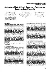
Fig. 2.

Example of missing state variables X,Y,Z

Even if we assume a single reason, the subgroup discovery problem can still exist. Figure 2 depicts a simple example. In this example, X,Y,Z and A-F are all state variables. Suppose the single reason can be explained by the rule XYZ. However, the state variables X, Y, Z are not included in the dataset. Instead, the state variables A-F are included. Suppose for each of state variable pairs AB, CD, and EF, the two state variables have an equal chance to appear in the simulation. The example shows that while the coverage of the rule XYZ is 100%, each of the eight rules, ACE, ACF, ADE, . . ., BDF, has only a coverage of 12.5%. If we do not allow a rule with low coverage, those rules would have been filtered out in the rule discovery process. Note that each of the eight rules, although their coverage is low, their precision should be 100%. The issue illustrated in Figure 2, although presented as a subgroup discovery problem, is in fact a feature selection problem, i.e. to select a proper set of state variables to build the dataset for rule learning. After all, if X, Y, Z are included in the dataset, the subgroup discovery would not be needed. C. Feature selection problem Suppose the true answer we are looking for is XYZ but in the dataset, the variable Z is missing. Let P (XY Z|XY ) be the conditional probability that XYZ appears in a simulation run

given that XY appears in the simulation run. The effectiveness of rule learning depends on this conditional probability. Assume the coverage and precision of XYZ are both 100%. First, the coverage of XY is also 100%. This is because XYZ should appear in all state vectors in Tf ail and consequently, XY should appear in all of them as well. If P (XY Z|XY ) ≈ 1, then the precision of XY should also be high. This is because if XY appears in many state vectors in Tpass , since P (XY Z|XY ) ≈ 1, XYZ would also appear in some state vectors in Tpass , contradicting the fact that XYZ does not appear in any state vector in Tpass , i.e. 100% precision. Therefore, we see that if P (XY Z|XY ) ≈ 1, missing a variable Z is not a serious problem. On the other hand, if P (XY Z|XY ) ≈ 0, then the precision of XY depends on the probability of XY’s occurrence in Tpass , which can be either high or low. In this case, Z is a critical variable and without it, it is hard to judge the quality of the rule XY by its precision. Based on the discussion, we see that if there is no missing state variable, the precision of a true answer should be 100%. However, 100% precision does not guarantee that there is no missing state variable. Furthermore, if the precision of a rule is not 100%, it is an indication of missing a state variable. Because the conditional probability such as P (XY Z|XY ) is unknown, it is usually difficult to evaluate the quality of a rule based on a precision that is significantly below 100%. For example, it is difficult to say that a 80%-precision rule is more likely to be the true answer than a 75%-precision rule. D. Ranking based on If ail (h) As discussed above, rule learning is to explore the two hypothesis rankings given by coverage and precision. Ideally, a rule learning run should provide two possible outcomes. First, some rules are accepted and presented to the user for manual investigation. Alternatively, no good rule is reported and the user should try a new run with a different set of state variables. The question is therefore how to set a hard threshold, in either coverage or precision or both, to discard hypotheses. The above discussion indicates that it is difficult to set a hard threshold based on coverage because multiple rules may coexist for explaining a bug. On the other hand, a hard threshold can be set based on precision because when the precision is not very high, it is difficult to compare the quality of two hypotheses based on their precision. Therefore, in our rule learning we discard all hypotheses that are below a hard threshold, for example 90%. The remaining hypotheses are ranked based on coverage. Because |Tf ail | is fixed, ranking based on coverage is the same as ranking based on If ail (h). E. If ail (h) Vs. |Tpass | Typically, we have |Tf ail |  |Tpass |. For example, |Tf ail | is on the order of tens or less while |Tpass | is on the order of tens of thousands or more. Hence, If ail (h) is a small number. Suppose the true answer is a rule r of length 3 (e.g. r =XYZ). Suppose |Tf ail | = j and If ail (r) = i. The significance of having If ail (r) = i can be illustrated with a simple example. Assume that j = 20. Also assume that the probability of each state variable appearing in a state vector is 0.5 (or 0.1) and these probabilities are mutually independent. Therefore, the probability of a hypothesis of length 3 appearing in a state vector is 0.125. Further assume that the total number of state variables is 200. With simple statistical simulation,

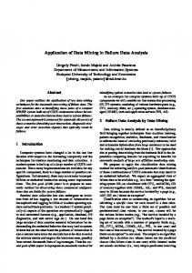
Figure 3 shows the expected number of hypotheses with If ail (h) ≥ i, for i = 2, . . . , 20. Observe that this number decreases almost exponentially as i increases. One can interpret the inverse of this expected number at If ail (h) = i as a measure of significance for the rule r with If ail (r) = i. In other words, a rule with a large If ail (r) is likely not by a random chance and hence, can be considered significant. The simple example shows that the significance of a hypothesis h increases almost exponentially as If ail (h) increases.

especially when the learning begins with a large |Tpass |. F. The length of a rule Suppose a rule r is a product of k variables. Suppose If ail (h) = i. Then, any rule rs consisting of a subset of these k variables would also have If ail (h) = i. However, the precision of rs should be equal to or less than the precision of r. This is because it is possible that rs appears in Tpass and r does not. In rule learning, if the precision of rs is the same as the precision of r, rs would be ranked higher than r because rs is more general (involves less variables). This strategy, i.e. when coverage and precision are both equal, a shorter rule is preferred, is also called Occam learning [8]. G. The overall methodology

Fig. 3.

Significance of a hypothesis h as If ail (h) increases

Suppose the analysis based on Tf ail generates k possible hypotheses of length 3. Suppose none of them is the true answer. Again, assume that the probability of each state variable appearing in a state vector is 0.5 (and 0.1) and there are in total 200 variables. With k = 1000, one can calculate the probability that at least one of the k hypotheses does not appear in any state vector in Tpass , i.e. based on 100% precision, this hypothesis would not be filtered out by the state vectors in Tpass . With k fixed at 1000, this probability decreases rapidly as |Tpass | increases and Figure 4 shows the probability is close to zero after a certain size of Tpass , i.e. all false positive hypotheses are likely to be filtered out with that size of Tpass . This simple example shows that with sufficient number of samples in Tpass , say 10K, all false positive hypotheses are likely to be filtered out (if they can be, statistically). If a false positive hypothesis cannot be statistically filtered out, it means that the probability of reaching the hypothesis by the constrained random tests is very low. In this case adding more passing state vectors (more tests generated based on the same test bench) might no longer be effective.

Fig. 5.

Overall methodology

Figure 5 depicts the rule discovery methodology. The run time of rule discovery depends on the size of the hypothesis space that further depends on two quantities: the number of state variables m and the maximum cardinality of a rule to consider. Typically, we would like to restrict m to be less than 100 and the cardinality less than 5. Figure 5 shows that the rule discovery process is iterative. From one iteration to the next, a user selects a different set of variables to build the hypothesis space. We assume that the M state variables are observed in the simulation traces. In a particular iteration, the investigation of a rule is based on the following rules of thumb: (1) A rule h with the highest If ail (h) is investigated first. (2) With everything else equal, a rule with the shortest length is investigated first. The investigation of a rule involves modifying the test bench according to the rule and generating new tests to observe if the frequency of hitting the bug is increased. If such frequency increase cannot be observed, the rule is considered invalid. V.

Fig. 6.

Fig. 4.

Expected # of false positive hypotheses not being filtered out

The two simple analyses above show that in general, having more positive state vectors is always more significant while adding more negative state vectors might not help much,

P ROCESSOR CORE RESULTS

Illustration of a platform

Figure 6 illustrates a platform architecture. A platform may comprise a number of processor cores, I/O cores, a platform MMU including cache, which are interconnected through some interconnect structure. A coherency manager is responsible for routing the transactions between cores and for ensuring data coherency in the system.

Verification can be divided into two parts, individual core verification and platform verification. For example, if the processor core is designed in house, verification of an individual processor core is required before platform verification. In platform verification, the focus is on the interconnection of cores. Therefore, coverage groups often are defined on the interconnect interfaces. Suppose a randomizer takes a test bench and generates a number of tests for processor verification. Let Tf ail be the set of state vectors where fails are observed in the simulation. Let Tpass be the set of the state vectors in the remaining cycles. We applied the proposed methodology to analyze the difference between Tf ail and Tpass .

Fig. 7.

State matrix view of a test

Figure 7 illustrates the hypothesis encoding scheme. We assume that the simulation trace observe all the microarchitecture state variables for the unit under analysis. For each analysis, a subset of p state variables are selected, S = {s1 , . . . , sp }. Given a test, simulation provides the state vector achieved at the end of each cycle. Note that in this state vector, ”1” means the state is present and ”0” means the state is not present. Suppose for a test we observe that a fail occurs at cycle j + 1. The state vector at cycle j+1 forms the positive state vector. The remaining state vectors are the negative state vectors. The set of positive state vectors becomes the set Tf ail . Similarly, the set of negative state vectors becomes the set Tpass .

Fig. 8.

Fig. 9.

Two examples for the experiments

signal lines. The first example concerns the functionality of handling a cache miss queue. The queue has eight entries. When the ith entry is filled, depending on the presence of other state variables, the entry will be forwarded. Each error is injected on the signal line indicating that the entry is waiting to be forwarded, i.e. the signal line is set when the entry is filled and waiting to be forwarded and is reset when the entry is forwarded. This waiting time usually is only one cycle. These errors are denoted as E0 , . . . , E7 . We used the test bench developed by the verification team targeting on this cache miss functionality in the LSU as the starting point to generate tests. The results labeled ”Initial” in Figure 10 show that with 400 tests, only E0 and E1 was excited in multiple cycles. Other errors were not excited. We applied the rule discovery to analyze the results based on E0 and E1 . A rule was found that was common to both errors. Since the rule was based on high-level machine states, it was not specific to a particular error. Instead, the rule explains under what condition, the miss queue is filled up. This rule was used to modify the test bench and 100 more tests were instantiated. The results labeled ”1st learning” show that all eight errors were excited at least once. The rule discovery was applied again with the new simulation data. A more precise rule was found to better model the forwarding functionality. 50 more tests were generated and the ”2nd learning” results show that all errors were excited in many cycles.

A positive state vector and its hypotheses

Given a positive state vector, a set of hypotheses can then be formed. For example, Figure 8 shows a positive state vector of 10 states. Since only states 3, 4, 6 and 8 are present, hypotheses are formed based on these four states. Others are ignored because we assume only monotonic rules as discussed before. With four states and maximum cardinality of 4, there are 24 − 1 = 15 hypotheses. Each hypothesis can then be evaluated for its coverage and precision. Suppose a rule is accepted for investigation. Then, finding the instructions causing each of the states in the rule is a relatively easy problem. One can trace back in time from the state vector to identify the corresponding instruction where a particular state is first present. The characteristics of those instructions together with the states provide user the information as how to modify the test bench or write a specific test to exercise the functionality that exposes the simulation fail. A. Example Results In the experiments we consider the load-store unit (LSU) of the processor core used in the commercial SoC platform. The processor core is a dual-thread low-power PowerPC compliant processor. The LSU is one of the most complex units to verify in the processor design. Figure 9 illustrates the two cases presented in this section. In each case, we manually inject stuck-at errors to selected

Fig. 10.

Improved error excitation - Example 1

Refer to example 2 in Figure 9. In this case, six errors E8 to E13 were injected. Again, we used the test bench developed by the verification team targeting on the functionality related to this module as the starting point. In the initial run, more than 30K tests were instantiated and simulated. None of the six errors were excited. However, with design knowledge we knew that six signal pairs (C, S0 ), (C, S1 ), . . ., (C, S5 ) could largely affect the functionality of the module. The rule discovery was applied to improve the coverage of these signal pairs, resulting in enhanced excitation of the errors. After learning based on the initial >30K tests and generating 1K new tests, Figure 11 (”1st learning”) shows that E11 to E13 could be excited in several cycles. E8 was excited once. The rule discovery was applied again by including the results from the 1K tests. The ”2nd learning” results show that all six errors could be excited in the simulation of 100 more tests.

99 − 13 = 86). As shown in Figure 13 (labeled ”2nd”) the remaining errors were excited in many cycles by the new tests.

Fig. 11.

Improved error excitation - Example 2

Note that in both experiments, a found rule was not specific to a particular error. Instead it was applicable to some or all errors in the same family. This was not surprising because rules were based on high-level machine states. They were useful for explaining the functionality of a given module rather than how to set a particular signal line in the module. VI. P LATFORM RESULTS By assuming each individual core is verified, platform verification focuses on verifying the interconnection. Figure 12 illustrates the idea.

Fig. 12.

Transaction view in platform verification

In platform verification, the focus is on the interface signals between the interconnects and a core. For example, a group may comprise a particular transaction type with combinations of attributes. From a core perspective there are two types of transactions, outgoing and incoming. Usually specific events of interest based on outgoing transactions are easier to hit because hitting those events only depends on supplying the required inputs to the core. Verification engineers usually have a good grasp of the behavior of the core and hence, it is relatively easy to write a test bench to produce desired outgoing transactions. Incoming transactions depend on the rest of the system. If an incoming transaction represents a response to an outgoing transaction, then whether the desired response can be observed or not depends on the system states and behavior of the rest of the system. It is much harder to prepare a test bench targeting on a particular incoming response. For the experiments run on the SoC platform, we therefore injected errors on the I/O Requester Ports comprising three similar I/O Requester Address Incoming (IRAIn) buses. The experiments include 99 injected stuck-at errors. In the original simulation of 2000 tests, only 13 errors were excited, as shown by the blue diamonds in Figure 13. Since the vertical axis is log-scale, only non-zero numbers are shown in the figure. In the case of platform, the state variables were system state variables that mostly describe the states of the coherency manager and the states of the platform cache. Two rules were found and used to modify the test bench. The 1st rule affected 9 of the 13 errors that had been originally excited (hence the 1st rule was common to these nine errors). The rule was used to produce 200 tests. As shown in Figure 13 (labeled ”1st”), the excitation frequencies of these nine errors were significantly increased. The 2nd rule affected the rest of the 86 errors (i.e.

Fig. 13.

Error excitation improvement of the two rules, 1st and 2nd

VII. C ONCLUSION In this work we explain how data mining can be applied in functional debug. We formulate the problem as a rule discovery problem and propose a rule discovery methodology. The methodology consists of two major components, feature selection and rule learning. The effectiveness of the rule learning depends on the feature selection. Because of this dependency, rule learning discards hypotheses without high precision and ranks the remaining hypotheses based on coverage. The methodology was applied in several experiments with injected errors. Results show that the proposed methodology allows effective rules to be found, which can be used to obtain more tests that excite the injected errors. Without a proper set of state variables (as the feature universe in Figure 5) to begin with, the proposed methodology might fail to discover any rule that is useful. Ensuring a proper set of state variables to begin rule discovery is a problem not addressed in this work and shall be left to future research. [1]

[2]

[3]

[4]

[5] [6]

[7] [8] [9]

[10]

[11]

R EFERENCES Y. Katz and et al. Learning microarchitectural behaviors to improve stimuli generation quality. In ACM/IEEE Design Automation Conference, pages 848 –853, 2011. W. Chen and et al. Simulation knowledge extraction and reuse in constrained random processor verification. In ACM/IEEE Design Automation Conference, 2013. S. Fine and et al. Coverage directed test generation for functional verification using bayesian networks. In Design Automation Conference, pages 286 – 291, june 2003. I. Wagner and et al. Microprocessor verification via feedback-adjusted markov models. Computer-Aided Design of Integrated Circuits and Systems, IEEE Transactions on, 26(6):1126 –1138, june 2007. G. Squillero. Microgp-an evolutionary assembly program generator. Genetic Prog. and Evolvable Machines, 6(3):247–263, Sept. 2005. K. Eder and et al. Inductive logic programming. chapter Towards Automating Simulation-Based Design Verification Using ILP, pages 154– 168. Springer-Verlag, Berlin, Heidelberg, 2007. Evangelos Triantaphyllou, edited by, Knowledge Discovery Approaches Based on Rule Induction Techniques Springer 2006. Michael J. Kearns and Umesh V. Vazirani. An Introduction to Computational Learning Theory, MIT Press, 1994. Onur Guzey, et. al. Extracting a Simplified View of Design Functionality Based on Vector Simulation. Lecture Note in Computer Science, LNCS, Vol 4383, 2007, pp. 34-49. N. Lavraˇc, B. Kavˇsek, P. Flach, and L. Todorovski. Rule induction for subgroup discovery with CN2-SD Journal of Machine Learning Research, 5:153–188, Dec. 2004. C. Zhang and S. Zhang, Association rule mining: models and algorithms. Springer, 2002.