IV International Workshop “Computational Problems of Electrical Engineering”
Zakopane 2002
On Blind Methods in Signal Processing Christian Jutten, Massoud Babaie-Zadeh, Shahram Hosseini Abstract— Blind methods are powerful tools when very weak information is necessary. Although many algorithms can be called blind, in this paper, we focus on blind source separation (BSS) and independent component analysis (ICA). After a discussion concerning the blind nature of these techniques, we review three main points: the separability, the criteria, the algorithms.
s -
F
x-
G
y -
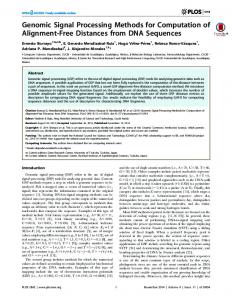
Fig. 1. General mixture and separation models.
I. Introduction Basically, the term blind in signal processing is associated to methods in which weak information about the signal is required. The methods are then efficient when no information is available. For instance, blind equalization techniques avoid to regularly send known sequences for identifying the channel; the blind techniques are then more efficient in term of communication rate. Another point of view is that blind techniques use criteria (or cost functions) which can be directly computed from the data. The algorithms are sometimes said unsupervised. For instance, in Kohonen’s self-organizing maps (SOM) [35], the criterion is a mean square error of quantization, which only depends on the data and on the quantifiers. In this paper, we focus on recent 1 techniques called blind source separation (BSS) or independent component analysis (ICA)[10], [30]. The main difference is that BSS concerns signals (with time properties) while ICA concerns more generally data. Anyway, BSS as well as ICA are driven by statistical independence which can be computed from the observations (i.e. blindly). In the context of signal processing, BSS is then a much more natural concept, and leads to many applications. BSS in instantaneous nonlinear mixtures consists in estimating n unknown sources from p observations x(t) = [x1 (t), x2 (t), · · · , xp (t)]T , which are an unknown mapping of n unknown sources s(t) = [s1 (t), s2 (t), · · · , sn (t)]T viewed by a set of p sensors: x(t) = F(s(t)), t = 1, . . . , T
The main assumption is the statistical independence of the sources. Although it is physically plausible, it is often considered as a strong assumption. In fact, it rather contests Gaussian assumption and relevance of decorrelation which have been so usual and convenient for many years, and are much more simpler to handle than non Gaussian and independence. The term blind emphasizes on the fact that (i) the sources are not observed, (ii) source distribution is unknown and a priori non Gaussian. Often, people claims that it is also blind since there is no information concerning the mapping F. As we will see in section II, strong assumptions on the mapping structure are used, and are actually necessary for insuring separability. Finally, it is often interesting to exploit very general signal properties, like temporal correlation (colored signals)[50], [9], [29] or non stationarity [38], [43]. In this review paper, we mainly discuss on three points: separability, independence criteria, algorithms. II. Separability The basic idea of BSS consists in estimating some inverse mapping G (Figure 1) of the transformation F such that each component of the output vector y(t) = G(x(t)), where y(t) = [y1 (t), y2 (t), · · · , yn (t)]T , is a function of one source. In the general case, the goal of separation is to obtain
(1)
where F is a one-to-one mapping. In the following, for sake of simplicity, we consider n = p. The authors are with the Signals and Images Laboratory (CNRS UMR 5083), INPG-LIS, 46 avenue F´ elix Viallet, 38031 Grenoble Cedex, E-mail:
[email protected]. C. Jutten is professor with University Joseph Fourier, Sciences and Techniques Institute of Grenoble (ISTG). This work has been partly funded by the European project BLISS (IST-1999-14190) and by the SASI project (ELESA-IMAG). 1 The first works have been published in 1985 in a conference [28] and then in a journal in 1991 [32], [19]
yi (t) = hi (sσ(i) (t)), i = 1, . . . , n
(2)
where hi is any invertible mapping which is associated to a residual distortion. Since the main assumption is the source independence, one suggests to estimate G, such that the estimated outputs y(t) = Gx(t) become statistically independent. The key question is the following: does output independence always insure separation, i.e. y(t) = s(t) ? 1
IV International Workshop “Computational Problems of Electrical Engineering”
A. Indeterminacies First, recall briefly the definition of independent random vector. Definition II-A.1: A random vector x is statistically independent if its joint probability Q density function (pdf) px (u) satisfies px (u) = i pxi (ui ), where pxi (ui ) are the marginal pdf of the random variables xi . Then, it is clear that the product of a permutation matrix P by any diagonal mapping both preserves independence and insures separability. Definition II-A.2: A one-to-one mapping H is called trivial, if it transforms any random vector s with independent components into a random vector with independent components. The set of trivial transformations will be denoted by T. Trivial mappings are then mapping preserving the independence property of any random vector. One can easily show that a one-to-one mapping H is trivial if and only if it writes as:
simply impossible by only using the statistical independence. In the conclusion of [21], Darmois clearly states: ”These properties [...] clarify the general problem of factor analysis by showing the large indeterminacies it presents as soon as one leaves the field, already very wide, of linear diagrams.”. B.1 A simple example A simple example derived from [47] is the following: suppose s1 ∈ R+ is a Rayleigh distributed variable with pdf ps1 (s1 ) = s1 exp(−s21 /2) and s2 ∈ [0, 2π) is uniform and independent of s1 . Consider the nonlinear mapping [y1 , y2 ] = =
B. Results from factor analysis In the general case, i.e. the mapping H has no particular form, a well known statistical result shows that the independence conservation constraint is not strong enough to insure the separability in the sense of equation (2). This result has been established, early in the 50’s, by Darmois [21] where he used a simple constructive method for decomposing any random vector as a non trivial mapping of independent variables. This result is negative, in the sense that it shows the existence of non trivial transformations H which still ”mix” the variables while preserving their statistical independence. Hence, for general nonlinear transformations and without constraints on the transformation model, source separation is 2
H(s1 , s2 ) [s1 cos(s2 ), s1 sin(s2 )]
(4)
which has a non diagonal Jacobian matrix µ J=
cos(s2 ) −s1 sin(s2 ) sin(s2 ) s1 cos(s2 )
¶ .
(5)
The joint pdf of y1 and y2 is:
Hi (u1 , u2 , . . . , un ) = hi (uσ(i) ), i = 1, 2, . . . , n (3) where hi are arbitrary functions and σ is any permutation over {1, 2, . . . , n}. This result establishes a link between the independence assumption and the objective of source separation. In fact, it becomes clear in the following that the source separation objective is, using the independence assumption, to impose that the global transformation H = G ◦ F is trivial. However, from (3) it is clear that sources can only be separated up to a permutation and a nonlinear function. In fact, for any invertible mappings F(x) = [f1 (x), . . . , fn (x)]T whose each component is a scalar nonlinear mappings fi (x) = Q fi (xi ), i = 1, . . . , n, it is evident that if p (u) = x i pxi (ui ), Q then pF(x) (v) = i pfi (xi ) (vi ). Moreover, this is not possible without imposing additional structural constraints on H, as we shall see in the next section.
Zakopane 2002
py1 ,y2 (y1 , y2 )
ps1 ,s2 (s1 , s2 ) |J| 1 −y 2 − y22 = exp( 1 ) 2π 2 −y 2 −y 2 1 1 = ( √ exp 1 )( √ exp 2 ) 2 2 2π 2π
=
The previous relation shows that the two random variables y1 and y2 are independent (although they are completely different of the sources) and Gaussian. Other examples can be found in the literature (see for example Lukacs [37]) or can be easily constructed. C. Specific model The previous negative result is due to the fact that we assume no constraints on the transformation H. Constraining the transformation H in a certain set of transformations Q can reduce these large indeterminacies. To characterize the indeterminacies for a specific model Q, one must solve the independence preservation equation which writes as: ∀E ∈ Mn R dF dF · · · dF s1 s2 sn = H(E) dFy1 dFy2 · · · dFyn(6) E
R
where Mn is a σ-algebra on Rn . Let P denote the set : P = {(Fs1 , Fs2 , . . . , Fsn ), / ∃H ∈ Q \ (T ∩ Q) : H(s) has independent components} (7)
IV International Workshop “Computational Problems of Electrical Engineering”
This set P contains all source distributions for which there exists a non trivial mapping H belonging to the model Q and preserving the independence of the s components. An ideal model will be such that P is empty and T ∩ Q contains the identity as a unique element. However, in general this is not fulfilled, we then say that source separation is possible when the sources ¯ the complement of P, sources distribution is in P, are then restored up to a trivial transformation belonging to T ∩ Q. C.1 Example: Linear models In the case of linear models, the transformation F is linear and can be represented by an n × n matrix A, the observed signals write then as e = As. Source separation consists then in estimating a matrix B such that y = Be = Hs has independent components. The set of linear trivial transformations T ∩ Q is the set of matrices equal to the product of a permutation and a diagonal matrix. Considering two linear functions of n independent random variables si , i = 1, . . . , n: x1 = a1 s1 + . . . + an sn x2 = b1 s1 + . . . + bn sn the Darmois-Skitovich theorem [21] states that, if ai bi 6= 0, independence of x1 and x2 implies that si is Gaussian. From this theorem, it is clear that the set P contains the distributions having at least two Gaussian components. We then conclude that source separation is possible whenever we have at most one Gaussian source, sources are then restored up to a permutation and a diagonal matrix [17].
A postnonlinear model (PNL) consists in nonlinear observations of the following form: n X
¾
e1
A
f1 .. . fn
en
x1 xn
g1 .. . gn
z1 zn
B
y1 . .. yn
-¾ Separating System -
Mixing System
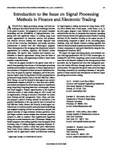
Fig. 2. The mixing-separating system for PNL mixtures.
As discussed before, the most important thing when dealing with nonlinear mixtures is the separability problem. First, we must think about the separation structure G which has as constraints: 1. Can invert the mixing system in the sense of equation (2): this constraint is quite obvious because that is what we want! 2. Be as simple as possible: In fact we want to reduce, in case we are successful, the residual distortions hi which are the blind spot of the independence assumption. By defining these two constraints, we have no other choice that selecting for the separating system G the mirror structure of the mixing system F (Fig. 2). E. Other separable non linear mixtures Due to the interesting Darmois’s result for linear mixtures, it is clear that nonlinear mixtures which could be reduced to linear mixtures with a simple mapping would be separable. E.1 A simple example As an example, one can consider multiplicative mixtures: xj (t) =
n Y
i sα i (t), j = 1, . . . , n
(9)
i=1
where si (t) are positive independent sources. Taking the logarithm leads to:
D. Separation of PNL mixtures
xi (t) = fi (
s1 . .. sn
Zakopane 2002
ln xj (t) =
n X
αi ln si (t), j = 1, . . . , n
(10)
i=1
aij sj (t)), i = 1, . . . , n,
(8)
j=1
Figure 2 shows what this model looks like. One can see that this model is a cascade of a linear mixture and a component-wise nonlinearity, i.e. acting on each output independently from the others. The nonlinear functions (distortions) fi are supposed invertible. Besides its theoretical interest, this model, belonging to the L-ZMNL2 family, suits perfectly for a lot of real world applications. For instance, such models can be found in sensors arrays [41], satellite and microwave communications [46], and in a lot of biological systems [36]. 2 L stands for Linear and ZMNL stands for Zero-Memory NonLinearity.
which is a linear model of the new independent random variables (since ln is monotonous) ln si (t). For instance, this type of mixtures can be used for modeling the gray-level images as the product of incident light and reflected light [25], or the cross-dependency between temperature and magnetic field in Hall silicon sensor. Considering in more details the latter example, the Hall voltage [45] is equal to: VH = kBT α
(11)
where α depends on the semiconductor type, since the temperature effect is related to the mobility of the majority carriers. In fact, in this model, the temperature T is positive, but the sign of the magnetic field B can vary. Then, using two types (N 3
IV International Workshop “Computational Problems of Electrical Engineering”
and P) of sensors, we have: VHN (t) = kN B(t)T αN (t) VHP (t) = kP B(t)T αP (t)
is due to the the fact that tan(a + b) is a function of tan a and tan b: (12) (13)
For simplifying the equations, in the following, we drop the variable t. Then, taking the logarithm: ln | VHN |= ln kN + ln | B | +αN ln T ln | VHP |= ln kP + ln | B | +αP ln T
(14) (15)
The above equations can be easily solved, even with simple decorrelation approaches. However, in that case, it is still simpler to directly compute the ratio of the two above equations : R=
VHN kN αN −αP = T VHP kP
(16)
which only depends on the temperature. Then, since R is a temperature reference (up to a scale factor), for separating the magnetic field, it is sufficient to estimate the parameter k such that VHN Rk becomes uncorrelated with R. We then deduce B(t) up to a mutiplicative constant. Finally, absolute estimations of B and T require calibration steps. E.2 Generalization to a class of mappings This extention of the Darmois-Skitovic theorem to more general nonlinear functions has been addressed in beginning of 70’s by Kagan et al. [33]. Their results have recently been revisited in the framework of source separation in nonlinear mixtures by Eriksson and Koivunen [25]. The main idea is to consider particular mappings F satisfying an addition theorem in the sense of the theory of functional equations. As a simple example of such a mapping, consider: s1 + s2 1 + s1 s2 s1 − s2 x2 = 1 − s1 s2 x1 =
where s1 and s2 are two independent random variables. Now, with the variable transformations u1 = tan−1 s1 and u2 = tan−1 s2 , the above nonlinear model becomes: x1 = tan(u1 + u2 ) x2 = tan(u1 − u2 ) Then, applying again the variable transformation on x1 and x2 leads to: v1 = tan−1 (x1 ) = u1 + u2 v2 = tan−1 (x2 ) = u1 − u2 which is now a linear mixture of two independent variables. As explained Kagan et al., the nice result 4
Zakopane 2002
tan(a + b) =
tan a + tan b 1 + tan a tan b
(17)
More generally, this property will hold provided than we consider mappings F satisfying an addition theorem like: f (s1 + s2 ) = F[f (s1 ), f (s2 )]
(18)
Let the range of u ∈ S be in the range [a, b], the basic properties required for the mapping (in the case of two variables, but extension is straightforward) are the following: • F is continuous at least separately for the 2 variables, 2 • F is commutative, i.e. ∀(u, v) ∈ S , F(u, v) = F(v, u), • F is associative, i.e. ∀(u, v, w) ∈ S3 , F(F(u, v), w) = F(u, F(v, w)) • It exists an identity element e ∈ S such that ∀u ∈ S, F(u, e) = F(e, u) = u −1 • ∀u ∈ S, it exists an inverse element u ∈ S −1 −1 such that F(u, u ) = F(u , u) = e In other words, denoting u ◦ v = F(u, v), it means that the set (S, ◦) is an Abelian group. Under this condition, Aczel [1] proved that it exists a monotonic and continuous function f : R → [a, b] such that: f (x + y) = F(f (x), f (y)) = f (x) ◦ f (y)
(19)
Clearly, applying f −1 (which exists since f is monotonic) to the above equation leads to: x + y = f −1 (F(f (x), f (y))) = f −1 (f (x) ◦ f (y)) (20) Using the above property (19), one can define a product ? with integer and extend it to real: f (cx) = c ? f (x)
(21)
or, taking f −1 and denoting f (x) = u, cf −1 (u) = f −1 (c ? u)
(22)
Then, for any constants c1 , . . . , cn and random variables u1 , . . . , un , the following relation holds: c1 f −1 (u1 )+. . . cn f −1 (un ) = f −1 (c1 ?u1 ◦. . .◦cn ?un ) (23) Finally, Kagan et al. stated the following theorem: Theorem II-E.1: Let u1 , . . . , un be independent random variables such that x1 = a1 ? u1 ◦ . . . ◦ an ? un x2 = b1 ? u1 ◦ . . . ◦ bn ? un are independent, and where the operators ? and ◦ satisfy the above conditions. Then, denoting f the
IV International Workshop “Computational Problems of Electrical Engineering”
function defined by the operator ◦, f −1 (ui ) is Gaussian if ai bi 6= 0. Practically, with such mixtures, the separation can be done in 3 steps: −1 • Apply f to the nonlinear observations for providing linear mixtures in si = f −1 (ui ) • Solve the linear mixtures in si by any BSS method • Restore the actual independent sources by applying ui = f (si ) If the function f is known, it is very easy. If f is not known, but if you suspect that the nonlinear mixtures has this particular form, you can constraint the separation structure to consist of identical nonlinear component-wise blocs (able to approximate f−1 ) followed by a linear matrix B able to separate sources in linear mixtures, and followed itself by identical non-linear component-wise blocs (which approximate f ) for restoring the actual sources. We remark that the 2 first blocs of the structure are identical (in fact, a little bit simpler, since all the nonlinear blocs are the same) to the separation structure of PNL mixtures. We can then estimate the independent distorted sources si with a PNL algorithm. Then, after computing f from the nonlinear bloc estimations, one can restore the actual sources. Finally, one can remark that the PNL mixture is close to these mappings. It is in fact more general since the nonlinear functions fi can be different. Other examples of such mappings are given in [33], [25], but realistic mixtures belonging to this class seems unusual. III. Independence criterion The previous section on separability points out that output independence, under a few structural constraints on the mixtures, is strong enough for driving the estimation of the separating structure G. In this section, we propose to study in more details the key concept of source separation: the statistical independence. A. Kullback-Leibler divergence Let y denote the output random vector, independence of y is defined by: Y py (u) = pyi (ui ) (24) i
but this relation between pdf’s is not easily tractable. A more convenient (scalar) measure of independence is derived from the Kullback-Leibler divergence 3 which measures the similarity between two distributions p and q of the same variable y: Z p(u) du (25) KL(p k q) = p(u) log q(u) 3 it
is not a distance, since it is not commutative
Zakopane 2002
It can be shown that KL(p k q) is greater of equal to 0, and the equality holds if and only if p = q. Then, independence can beQ computed like the KL divergence between py and i pyi : Z Y py (u) KL(py k pyi ) = py (u) log Q du i pyi (ui )) i (26) Q which vanishes if and only if py = i pyi , i.e. y is independent. This quantity is often called mutual information and denoted I(y) [20]. Defining H(y) and H(yi ) the joint and marginal entropies, respectively: Z H(y) = − py (u) log py (u)du Z H(yi ) = − pyi (ui ) log pyi (ui )dui the mutual information can be written: Y X I(y) = KL(py k pyi ) = H(yi ) − H(y) (27) i
i
B. Estimating equations Due to MI properties, estimation of the separation structure can then be obtained by minimizing MI. Although the general relation (27) can be directly derived for providing the estimation equations, usually, this equation is simplified taking into account the separation structure. B.1 MI optimization for linear mixtures For linear mixtures, F is a n×n invertible matrix F = A, and the separation structure is constrained to be a n × n invertible matrix B. Since y = Bx and x = As, the relation between x and y pdf’s writes: py (u) = px (B−1 u)/ | det B | and the MI becomes: X I(y) = H(yi ) − H(x) − log | det B |
(28)
(29)
i
Then MI optimization with respect to the separation matrix B requires the gradient: ∂ X ∂I(y) = H(yi ) − B−T ∂B ∂B i
(30)
P Finally, since yi = i bik xk , the derivative of MI with respect to B is: ∂I(y) = EΨy xT − B−T ∂B
(31)
where E denotes mathematical expectation and Ψy = [Ψy1 . . . Ψyn ]T , whose component Ψyi is the score function of yi defined as: Ψyi (yi ) = −
p0y ∂ log pyi (yi ) = − i (yi ) ∂yi p yi
(32) 5
IV International Workshop “Computational Problems of Electrical Engineering”
After right multiplication by BT , one gets the estimation equation: EΨy yT − I = 0
(33)
where I is the n × n identity matrix. The expression (33) points out the relevance of score functions. In fact, the complete knowledge on each estimated sources yi is summarized in the score function Ψyi . Moreover, the score functions are related to the optimal statistics. In fact, if yi is zero-mean Gaussian with unit variance, its score function is Ψyi (yi ) = yi , and the estimating equation entries reduce to Eyi yj = δij , i.e. simple decorrelation equations (for i 6= j). Conversely, if yi is non Gaussian, its score function is a nonlinear function and estimating equation entries Eψyi (yi )yj = δij involve cancellation of higher (than 2) order statistics. B.2 MI optimization for nonlinear mixtures For nonlinear mixtures, we assume that F and G are both n-variate invertible mappings. Since y = G(x) and x = F(s), the relation between x and y pdf’s writes: py (u) = px (G −∞ (u))/ | det JG | and the MI becomes: X I(y) = H(yi ) − H(x) − log | det JG |
(34)
(35)
i
In the special case of PNL mixtures, MI simplifies to: X I(y) = H(yi ) − H(x) − log | Πi gi0 (xi ) | i
Ψy = [Ψy1 . . . Ψyn ]T whose component Ψyi is the marginal score function of yi defined as in (32) T • Φy (y) = [Φ1 (y) . . . Φn (y)] whose component Φi (y) is the joint score function of y defined as: •
Φi (y) = −
∂ log py (y) ∂yi
(39)
• βy , Ψy − Φy is the difference between marginal and joint score functions of y, and we call it SFD (Score Function Difference). After right multiplication by BT , one gets the estimation equation:
EΨy yT − I = 0
or
Eβy yT = 0
(40)
B.4 MI optimization for linear convolutive mixtures For linear convolutive mixtures, F is a n × n invertible matrix of filters F = A(z). For instance, if A(z) is a finite impulse response filter of order L, the observation is: x(k) = [A(z)]s(k) =
L X
Al s(k − l)
(41)
l=0
The separation structure is then constrained to be a n × n invertible matrix of filters G = B(z): y(k) = [B(z)]x(k) =
p X
Bl x(k − l)
(42)
l=0
Unfortunately, due to the filter, there is no simple relationship between x and y pdf’s. So, we have to derive the basic MI equation X H(yi ) − H(y) (43) I(y) = i
− log | det B | (36) Consequently, MI minimization leads to two equations for estimating the nonlinear part and the nonlinear part of the separating structure. Equations related to linear part is similar to (33). Conversely, denoting zi = gi (xi ), equations related to the nonlinear part is: X E[ bij Ψyi (yi ) | zj ] = Ψzj (zj ), j = 1, . . . , n (37) i
Again, one remarks that optimal minimization of MI requires knowledge of the score functions. B.3 Direct MI optimization POne also can optimize directly the MI I(y) = i H(yi ) − H(y) with respect to B: ∂I(y) = EΨy xT − EΦy xT = Eβy xT ∂B where • E denotes mathematical expectation, 6
Zakopane 2002
(38)
In fact, it can be shown [5] that up to first order terms, we have: I(y + ∆) − I(y) = E∆T βy
(44)
where ∆ stands for a ‘small’ random vector. This equation proposes that SFD is the stochastic gradient of the mutual information. Moreover, it must be noted that signal independence in convolutive mixtures means stochastic process independence. Then, we have to take into account independence between delayed signals. For sake of simplicity, consider only the above term and derive it with respect to Bk . To do that, let ˆ k = Bk + ε, where ε represents a ‘small’ matrix. B Then we have: y ˆ(n) , [B(z)]x(n) = y(n) + εx(n − k)
(45)
Now by combining the above equation with (44), and doing a little algebra, we find that: ∂I(y(n)) = Eβy (y(n)) xT (n − k) ∂Bk
(46)
IV International Workshop “Computational Problems of Electrical Engineering”
However, we need the gradient of the MI of the delayed versions of outputs, that is, the gradient of I(y1 (n), y2 (n − m)) (in the case of 2 mixtures of 2 sources). This gradient can be found with a similar approach, which is: ∂I(y1 (n), y2 (n − m)) = Eβm (n) xT (n − k) (47) ∂Bk where β(n) is obtained by the following procedure: µ ¶ µ ¶ y1 (n) y1 (n) Shift SFD −−−→ −−−→ y2 (n) y2 (n − m) µ ? ¶ µ ¶ β1 (n) β1? (n) Shift back −−−−−−−→ , βm (n) β2? (n) β2? (n + m) (48) Hence, the complete set of estimating equations is: Eβm (n) xT (n − k) = 0
, ∀k, m
(49)
It is equivalent to using the separation criterion: X J= I(y1 (n), y2 (n − m)) (50)
Zakopane 2002
C.1 Separating structure with pre-whitening Many methods [15], [31] are based on the following decomposition of the separation matrix B: B = UW
where W is a whitening matrix and U is an orthogonal matrix. Let us denote z = Bx, z is whitened means that it satisfies EzzT = I. The decomposition also forces the output variance to be equal to 1 (since U is orthogonal, y = Uz satisfies EyyT = I) which relaxes the scale indeterminacies. Then, the MI of the outputs can be written: I(y) =
X
B.5 MI optimization for convolutive PNL (CPNL) mixtures The approaches of the sections III-B.2 and IIIB.4 can be combined for separating convolutive PNL (CPNL) mixtures [4]. In these mixtures, a linear convolutive mixture is followed by componentwise invertible non-linearities (corresponding to sensors). The separation criterion is as (50). This results in the same estimating equation (49) for estimating the convolutive part, and the estimating equation: E[αi | zi ] = 0,
i = 1, 2
(54)
Moreover, after computing (at the second order) the whitening matrix W, the joint entropy H(z) is a constant and, since the determinant of an orthogonal matrix is equal to 1, MI reduces to: I(y) =
X
H(yi ) + cst
(55)
i
Minimizing the MI is then equivalent to minimizing the sum of the marginal output entropies. It is well known that, for random variables with a given variance, the entropy is maximal for Gaussian variables. Consequently, since output variance is constant EyyT = I, (55) can be seen as a measure of gaussianity. In other words, minimizing MI is equivalent to minimizing the gaussianity of the estimated sources. C.2 Infomax Another approach, initially proposed by Bell and Sejnowski [7], consists in computing transformed output signals z, obtained by component-wise invertible nonlinear mapping Fyi : zi = Fyi (yi ), i = 1, . . . , n
(56)
(51)
for non-linear part. In this equation α = (α1 , α2 )T is defined by: · µ ¶¸ 1 βm (n) BTk βm (n + k) = BT z k=0 (52) where βm (n) is given by (48). α(n) ,
H(yi ) − H(z) − log | det U |
i
m
However, minimizing J is very cost consuming. Hence, in practice, we use I(y1 (n), y2 (n − m)), but in each iteration a (randomly chosen) different m is used [3].
(53)
p X
C. Criteria for constrained separation structures As we explained, constraining the separation structures can reduce the indeterminacies and even insuring separability. It also can have a direct influence on the independence criterion. In this section, we show how the MI is modified by two usual constraints.
where Fyi is the cumulative probability density function of the random variable yi . Since MI is not modified by component-wise invertible mappings, one can write: X I(z) = I(y) = H(zi ) − H(z) (57) i
Each transformed variable zi being uniformly distributed in [0, 1], MI becomes: I(z) = I(y) = cst − H(z)
(58)
Consequently, minimizing the MI is equivalent to maximazing the joint entropy of the transformed outputs z: the algorithm associated to this constraint is called Infomax. 7
IV International Workshop “Computational Problems of Electrical Engineering”
D. Estimating the estimation equations As we explained after deriving the gradient of MI for various mixtures in III-B, the key information concerning the estimated sources is their score functions, i.e the opposite of the derivatives of their logdensities. If the score functions are a priori chosen, the statistics involved in the estimating equations are not optimal. However, for estimating the separation matrix (in linear mixtures), one can remark that a very accurate estimation of score functions is not necessary. In fact, the estimating equation (33) leads to the set of equations: Eψyi (yi )yj = 0, i 6= j
(59)
since diagonal terms of (33) are only normalization equations. If the yi ’s are statistically independent zero-mean variables (i.e. Eyj = 0, i = 1, . . . , n), it is clear that: Eψyi (yi )yj = Eψyi (yi )Eyj = 0, i 6= j
(60)
even with a poor estimation equation of ψyi . However, a coarse estimation of the score function leads to slower convergence or even to algorithm divergence. Conversely, solving equation (37), associated to nonlinear part estimation, requires an accurate estimation of the score functions which appear both in left and right side terms on the equation. A comparison between 4-th order estimations obtained with a Gram-Charlier expansion and a MSE criterion is presented in [47]. It emphasizes on the weak accuracy of 4-th Gram-Charlier expansion, and explained the difficulties for separating hard nonlinear mixtures when deriving MI with this expansion [53] . In any case, the score function estimation is very important for determining the optimal statistics and for designing efficient separation algorithms. D.1 Estimating the score function from the density Since the score function is related to the probability density function, a natural approach is to first estimate the pdf (or the logarithm of the pdf), and then to deduce the score function with: ψˆyi (yi ) =
pˆ0yi (yi ) pˆyi
(61)
Various methods for estimating pdf’s are very usual in statistics. A first approach is based on GramCharlier or Edgeworth expansions of the density pyi around Gaussian [34]. Without considering details, we can note that these expansions explicitely involve high-order cumulants. 8
Zakopane 2002
Another approach is based on kernel estimator of pdf’s [26]: pˆX (u) =
T 1X Kh (u − Xi ) T i=1
(62)
where the Xi ’s are samples of the random variable X, and h is the bandwidth which determines the width of each kernel. Larger is h, smoother is the estimation. Of course, h depends on the sample number T . Experimentally, it seems that an optimal choice of h, based on cost-computing crossvalidation, is not required, and a simple rule [47] is efficient. D.2 Direct estimation of score functions Score functions can also be directly estimated for minimizing a mean square error. In fact, denoting ˆ ψ(w, u) a parametric estimation of ψ(u), and using the definition of the score function, the MSE criterion: J(w) =
1 ˆ E(ψ(w, u) − ψ(u))2 2
(63)
leads to the gradient: ∂J(w) ∂ ψˆ ∂ 2 ψˆ ˆ = E[ψ(w, u) (w, u) + (w, u)] ∂w ∂w ∂u∂w (64) The above gradient can be used for estimating any type of model, e.g. based on a basis of nonlinear functions [44], [12], on neural networks [47], or on other nonlinear models like splines, polynomials, etc. E. Contrast functions Constrast functions, initially defined by Donoho [24] for blind deconvolution, have been introduced by Comon [16], [17] in the framework of blind source separation. E.1 Definition Basically, a contrast function is a real function of a distribution y, which should be minimal if y is independent. For linear mixtures, the definition is the following: Definition III-E.1: A function φ[s] of the distribution s is a contrast function if, for any matrix C and any random variable s, φ[Cs] ≥ φ[s], with equality if and only if C = PD, where P and D are a permutation matrix and a diagonal matrix, respectively. The above definition has been extended to convolutive mixtures [18] or nonlinear mixtures, PD being replaced by trivial filters PD(z) or by trivial nonlinear mappings hi (sσ(i) ). Contrast functions are then good candidates for driving source separation algorithms, since they should be minimum when source separation is achieved.
IV International Workshop “Computational Problems of Electrical Engineering”
Then, a main issue is to find contrast functions as simple as possible. E.2 A few examples First, it is easy to verify that MI is a contrast function. However, this function is complex enough, since it requires the estimation of score functions. Conversely, it is easy to see that EyyT is not a contrast, which is not surprising since we know that second order statistics does not generally insure independence. In fact, adding high order statistics up to order 3 or 4, can lead to the simplest contrast functions. However, these contrast functions are often associated to restrictive conditions on the sources. For instance, the simple function: φ[y] = ²
n X
| Cumyi , yi , yi , yi |
(65)
i=1
is a contrast for sources with the same kurtosis sign ². If not, the algorithm diverges! Moreover, simpler contrasts can be derived under structural constraints. For instance, the decomposition of the separation matrix B = UW leads to the class of orthogonal contrasts. An detailed and very interesting discussion on contrast functions can be found in [10]. F. Performance In the case of linear mixtures, the choice of the contrast functions influence convergence speed, but asymptotic performance is weakly dependent of the contrast function, provided than the algorithm converges. On the contrary, Cardoso proved [10] that asymptotic performance is penalized by using a prewhitening. IV. Using time structure When the sources are time signals, they may contain more structure than simple random variables. This time structure (correlation, non-stationarity, etc.) may be used for improving the estimation. It may even make the separation possible in cases where the basic ICA methods fail, for example, if the sources are Gaussian but correlated or nonstationary over time. A. Correlated sources The time dependence between successive samples of the signals may be explored in different manners. While simple second order approaches consider only the time-lagged covariance matrices, more complicated methods may consider the higher order timelagged statistics or even the joint pdf of successive time samples, for example using Markov models. A.1 Second order approaches It is known that the instantaneous (zero-lagged) covariance matrix does not contain enough param-
Zakopane 2002
eters for solving the ICA problem up to classical indeterminacies. If x(t) is the vector of observations (mixtures), there exists an infinity of different matrices V so that the components of the vector y(t) = Vx(t) are decorrelated. This is why in basic ICA, we must use higher order statistics. However, if the sources are correlated in time, using the timelagged covariance matrices, ª © Cxτ = E x(t)x(t − τ )T ,
(66)
we can obtain the complementary information for separating the sources without using higher order statistics. In the simplest case, we can find a separating matrix which diagonalizes both the instantaneous and the first lagged covariance matrices. It has been shown that such a matrix reconstructs the sources up to classical indeterminacies, if the first lagged covariances are different for all the sources. The algorithms presented in [49] and [39] are examples of first lagged covariance diagonalization algorithms. The method may be extended by using the joint diagonalization of several time lagged covariances [9], [55], [22]. A good review about second order approaches can be found in chapter 18 of [30]. The main drawback of these methods is that they are not able to separate the sources with same power spectra. A.2 Markov models Another possibility is to exploit the complete time dependence structure of the sources, which is modeled as q-th order Markov sequences for simplicity. Such models can be completely characterized by the joint probability density of q + 1 successive samples of each source. Then, a quasi maximum likelihood (ML) method may be used for estimating the separating matrix B. Basically, the ML method consists in maximizing the joint pdf of all the T samples of all the components of the vector x (all the observations), with respect to B. We denote this pdf: f (x1 (1), · · · , xn (1), · · · · · · , x1 (T ), · · · , xn (T )) (67) Under the assumption of source independence, this function is equal to: n Y 1 T ) fs (eT Bx(1), · · · , eTi Bx(T )) | det(B−1 )| i=1 i i (68) where fsi (.) represents the joint density of T samples of the source si and ei is the i-th column of the identity matrix. We suppose now that the sources are q-th order Markov sequences, i.e.:
(
fsi (si (t)|si (t − 1), · · · , si (1)) = fsi (si (t)|si (t − 1), · · · , si (t − q))
(69) 9
IV International Workshop “Computational Problems of Electrical Engineering”
Using (69), equation (68) reduces to: (
n Y 1 T ) [fs (eT Bx(1), · · · , eTi Bx(q)) | det(B−1 )| i=1 i i T Y
fsi (eTi Bx(t)|eTi Bx(t − 1), · · · ,
t=q+1
eTi Bx(t − q))] (70) Taking the logarithm of (70), one obtains the loglikelihood function which must be maximized to estimate the separating matrix B: L1 = T log(| det(B)|) +
n X
[log(fsi (eTi Bx(1), · · · ,
i=1
eTi Bx(q))) +
T X
log(fsi (eTi Bx(t)|eTi Bx(t − 1)
t=q+1
, · · · , eTi Bx(t − q)))] (71) In practice, the density functions of the true sources, fsi in (71), are unknown and must be replaced with the estimated density functions of reconstructed sources, fyi . Then, the criterion (71) becomes asymptotically: L2 = − log | det(B)| −
n X
E[log fyi (yi (t)|yi (t − 1),
i=1
· · · , yi (t − q))] (72) To estimate the matrix B, we need to compute the gradient of the criterion (72) with respect to B: n
∂L2 ∂ X log fyi (yi (t)|yi (t − 1) = −B−T − E[ ∂B ∂B i=1 , · · · , yi (t − q))] (73) Using some computations, the following estimating equations can be derived (for i 6= j): q X E[ ψy(l) (yi (t)|yi (t − 1), · · · , yi (t − q))yj (t − l)] = 0 i l=0
(74) which determine B up to a scaling and a per(l) mutation. In these equations, ψyi (yi (t)|yi (t − ∂ 1), · · · , yi (t − q)) = − ∂yi (t−l) log fyi (yi (t)|yi (t − 1), · · · , yi (t−q)) is the l-th component of the conditional score function, which is a vector of size q + 1. The conditional score functions are estimated using a kernel method. The algorithm is theoretically able to separate every linear mixture unless there are at least two Gaussian sources with same spectral densities. It 10
Zakopane 2002
provides an asymptotically efficient (unbiased, minimum variance) estimation of the separating matrix. It is however rather slow because estimating the conditional score functions is time-consuming. B. Non stationary sources The non stationarity of the sources can be also exploited to achieve separation. In particular, the non stationarity of the source variances has been used for separating Gaussian or non Gaussian sources with no temporal correlation. The simplest approach consists in considering the second order statistics, i.e. correlation between different sources. It has been shown [38] that if σi2 /σj2 are not constant for ∀i 6= j, a matrix B so that the components of y(t) = Bx(t) are uncorrelated at every time instant t, is a separating matrix. A practical algorithm consists in estimating the instantaneous covariance matrix on short time intervals over which the signals are supposed stationary. Because of the non stationarity of the sources, this matrix depends on the interval label. Thus, an adaptive algorithm may be used for diagonalizing this matrix on all the intervals. Other algorithms based on the non stationarity of the source variances can be found in the literature [8], [43]. From a theoretical point of view, in [43], Pham and Cardoso derived a Gaussian form of the MI in that case and proved very interesting properties of the criterion and of the associated algorithms. Practically, the algorithms are still based on joint diagonalization of covariance matrices, computed on successive time windows. V. Algorithms Many algorithms have been developed in the literature since 1985 (see in [30] for a review and most of the references). However, a few principles are very important and will be pointed out in this section. A. Equivariant algorithms The convergence speed of the first algorithms [28], [14] was depending on the mixture A. For overcoming this problem, Cichocki et al. proposed the first robust (equivariant 4 ) algorithm [13]. Independently, instead additive algorithms of the form B ← B − µ ∂J(y) ∂B , Cardoso introduced algorithms (for separating linear mixtures) based on multiplicative updates: B ← (I − µOB (J))B. Leftmultiplying this relation by A leads to: C ← (I − µOB (J(Cs))C
(75)
which clearly does no longer depend on the mixing matrix A. The algorithm is then based on the differential of J((I+ε)y), which has been derived independently by Cardoso and Laheld [11], and Amari 4 The word ”equivariant” has been introduced later by Cardoso and Laheld
IV International Workshop “Computational Problems of Electrical Engineering”
et al. [2], under different names, relative and natural gradients, respectively. B. Joint diagonalization In the previous section, we explained how, relaxing the i.i.d. assumption, with colored signals (first ”i” no longer holds) or with non stationary sources (”i.d.” non longer holds), MI (or ML) criterion leads to joint diagonalization of variance-covariance matrices. Then, a special interest has been focused on the designing of efficient joint diagonalization algorithms [52], [42], [54]. We especially recommend the algorithm proposed by Pham [42] for its simplicity, its high speed and its performance. C. Minimizing Mutual Information Finally, deriving quasi-optimal 5 algorithms minimizing MI is possible. The algorithm is then based on (i) the estimations ψˆyi of the score functions of the estimated sources yi , (ii) the estimation of the separation structure with estimating equations where the true score functions ψyi are replaced by the estimations ψˆyi [44], [12], [47]. An interactive demonstration of such algorithms, developed in Java (and the Matlab codes), is available on the Web page: http://www.lis.inpg.fr/demos/sep_sourc/ ICAdemo/index.html. It shows the efficacy of these algorithms for separating linear as well as post-nonlinear mixtures and for achieving blind deconvolution and blind inversion of Wiener systems.
Zakopane 2002
However, this new and very active field of research emphasizes still many challenging questions. As examples, designing efficient methods for separating sources (i) from realistic MIMO convolutive mixtures, (ii) from noisy mixtures, (iii) from mixtures with more sources than sensors, (iv) from nonlinear mixtures, are among the most relevant. The development of independent component analysis (ICA) for sparsely representing complex data like speech or images [23], [51] (with a basis whose elements are as independent as possible) and for understanding how the brain could sparsely code such complex signals [6], [27], [40], is also an promising topics of research. Finally, although promising applications has been developed in many fields (EEG and MEG signal processing, communications, smart sensor array design, ”cocktail party” processing, etc.), a lot of works remains to do for considering these methods as an usual tools in signal processing or statistics toolboxes. References [1] [2]
[3]
[4] [5]
VI. Conclusion In this paper, we reviewed a few key points on the blind source separation and independent component analysis. Concerning the separability, one has to remember that statistical independence cannot generally insures separation. In fact, a large class of non diagonal mapping preserves independence, and adding structural constraints is a good approach for restricting the solutions to trivial mappings. The methods are also strongly related to blind deconvolution or blind inversion of Wiener (nonlinear) systems: it is easy to see that the problems are very similar to source separation in linear or postnonlinear mixtures, respectively [48]. These blind methods, based on statistical independence, are driven by the minimization of the mutual information (MI). Simple approximations of the MI leads to algorithms generally having a few restrictions. Conversely, approximations based on score function estimation can provide quasi-optimal algorithms.
[6]
5 ’quasi’ since they used estimated score functions instead the true (unknown) ones
[16]
[7] [8] [9]
[10] [11] [12]
[13] [14] [15]
J. Aczel. Lectures on functional equations and their applications. Academic Press, New-York, 1966. S. Amari, A. Cichocki, and H. Yang. A new learning algorithm for blind signal separation. In Advances in Neural Information Processing Systems, pages 757– 763, Denver (Colorado), December 1996. M. Babaie-Zadeh, C. Jutten, and K. Nayebi. Separating convolutive mixtures by mutual information minimization. In Proceedings of IWANN 2001, Granada, Spain, 2001. M. Babaie-Zadeh, C. Jutten, and K. Nayebi. Separating convolutive post non-linear mixtures. In Proceedings of ICA 2001, San Diego (California, USA), 2001. M. Babaie-Zadeh, C. Jutten, and K. Nayebi. Differential of mutual information function. IEEE Signal Processing Letters, 2002. Submitted in May. H. B. Barlow. Unsupervised learning. Neural Computation, 1:295–311, 1989. A. Bell and T. Sejnowski. An information-maximization approach to blind separation and blind deconvolution. Neural Computation, 7(6), 1995. A. Belouchrani and M. Amin. Blind source separation based on time-frequency signal representation. IEEE Trans. on Signal Processing, 46(11):2888–2897, 1998. A. Belouchrani, K. Abed Meraim, J. F. Cardoso, and E. Moulines. A blind source separation technique based on second order statistics. IEEE Trans. on Signal Processing, 45(2):434–444, 1997. J.-F. Cardoso. Blind signal separation: statistical principles. Proceedings IEEE, 9(10):2009–2025, 1998. J.-F. Cardoso and B. Laheld. Equivariant adaptive source separation. IEEE Trans. on SP, 44(12):3017– 3030, 1996. N. Charkani and Y. Deville. Optimization of the asymptotic performance of time-doamin convolutive source separation algorithms. In Proc. ESANN, pages 273– 278, Bruges, Belgium, April 1997. A. Cichoki, Unbehauen R., and E. Rummert. Robust learning algorithm for blind separation of signals. Electronics Letters, 30(17):1386–1387, 1994. P. Comon. S´ eparation de m´ elanges de signaux. In Actes du XII ` eme colloque GRETSI, pages 137–140, JuanLes-Pins (France), Juin 1989. P. Comon. Separation of sources using higher-order cumulants. In SPIE Vol. 1152 Advanced Algorithms and Architectures for Signal Processing IV, San Diego (CA), USA, August 8-10 1989. P. Comon. Independent component analysis. In J.-L. Lacoume, M. A. Lagunas, and C. L. Nikias, editors, In-
11
IV International Workshop “Computational Problems of Electrical Engineering”
[17] [18] [19] [20] [21] [22] [23]
[24] [25] [26] [27] [28]
[29]
[30]
[31] [32] [33]
[34] [35] [36] [37] [38] [39] [40] [41]
12
ternational Workshop on High Order Statistics, pages 111–120, Chamrousse, France, July 1991. P Comon. Independent component analysis, a new concept ? Signal Processing, 36(3):287–314, 1994. P Comon. Contrasts for multichannel blind deconvolution. IEEE Signal Processing Letters, 3(7):209–211, 1996. P. Comon, C. Jutten, and J. H´ erault. Blind separation of sources, Part II: Statment problem. Signal Processing, 24(1):11–20, 1991. T. M. Cover and J. A. Thomas. Elements of Information Theory. Wiley Series in Telecommunications, 1991. G. Darmois. Analyse des liaisons de probabilit´ e. In Proceedings Int. Stat. Conferences 1947, volume III A, page 231, Washington (D.C.), 1951. S. Degerine and R. Malki. Second order blind separation of sources based on canonical partial innovations. IEEE Trans. on Signal Processing, 48(3):629–641, 2000. D. L. Donoho. Nature vs. math.:interpreting independent component analysis in light of computational harmonic analysis. In Proceedings of ICA 2000, Helsinki (Finland), 2000. D.L. Donoho. On minimum entropy deconvolution. In Applied Time Series Analysis II, pages 565–608, Tulsa, 1980. J. Eriksson and V. Koivunen. Blind identifiability of class of nonlinear instantaneous ICA models. In EUSIPCO 2002, Toulouse (France), September 2002. W. H¨ ardle. Smoothing Techniques, with implementation in S. Springer-Verlag, 1990. G. H. Harpur and R. W. Prager. Development of low entropy coding in a recurrent network. Networks, 7:277– 284, 1996. J. H´ erault, C. Jutten, and B. Ans. D´ etection de grandeurs primitives dans un message composite par une architecture de calcul neuromim´ etique en apprentissage non supervis´ e. In Actes du X ` eme colloque GRETSI, pages 1017–1022, Nice (France), 20-24 Mai 1985. S. Hosseini, C. Jutten, and D. T. Pham. Blind separation of temporally correlated sources using a quasimaximum likelihood approach. In Proceedings of ICA 2001, San Diego (California, USA), 2001. A. Hyv¨ arinen, J. Karhunen, and E. Oja. Independent component analysis. Adaptive and Learning Systems for Signal Processing, Communications, and Control. John Wiley, New York, 2001. A. Hyv¨ arinen and E. Oja. A fast fixed-point algorithm for independent component analysis. Neural Computation, 9(7):1483–1492, 1997. C. Jutten and J. H´ erault. Blind separation of sources, Part I: an adaptive algorithm based on a neuromimetic architecture. Signal Processing, 24(1):1–10, 1991. A.M. Kagan, Y.V. Linnik, and C.R. Rao. Extension of darmois-skitovic theorem to functions of random variables satisfying an addition theorem. Communications in Statistics, 1(5):471–474, 1973. M. Kendall and A. Stuart. The Advanced Theory of Statistics, Distribution Theory, volume 1. Griffin, 1977. T. Kohonen. Self-Organizing Maps. Springer, 1995. M.J. Korenberg and I.W. Hunter. The identification of nonlinear biological systems: LNL cascade models. Biological Cybernetics, 43(12):125–134, December 1995. E. Lukacs. A characterization of the Gamma distribution. Ann. Math. Statist., (26):319–324, 1955. K. Matsuoka, M. Ohya, and M. Kawamoto. A neural net for blind separation of nonstationary signals. Neural Networks, 8(3):411–419, 1995. L. Molgedey and H. G. Schuster. Separation of a mixture of independent signals using time delayed correlation. Physical Review Letters, 72:3634–3636, 1994. B. A. Olshausen and D. J. Field. Emergence of simplecell receptive field properties by learning a sparse code for natural image. Nature, 381:607–609, 1996. A. Parashiv-Ionescu, C. Jutten, A.M. Ionescu, A. Chovet, and A. Rusu. High performance magnetic field smart sensor arrays with source separation. In MSM 98, pages 666–671, Santa Clara (California, USA), April 1998.
Zakopane 2002
[42] D. T. Pham. Joint approximate diagonalization of positive definite hermitian matrices. SIAM Journal on Matrix analysis and Application, 2001. To appear. [43] D. T. Pham and J. F. Cardoso. Blind separation of instantaneous mixtures of non stationary sources. In Int. Workshop on Independent Component Analysis and Blind Signal Separation, ICA’2000, pages 187–193, Helsinki (Finland), 2000. [44] D. T. Pham, Ph. Garat, and C. Jutten. Separation of a mixture of independent sources through a maximum likelihood approach. In Proc. European Signal Processing Conf. EUSIPCO 92, pages 771–774, Brussels (Belgium), August 1992. [45] R. S. Popovic. Hall-effect devices. Adam Hilger, Bristol, 1991. [46] S. Prakriya and D. Hatzinakos. Blind identification of lti-zmnl-lti nonlinear channel models. IEEE trans. S.P., 43(12):3007–3013, December 1995. [47] A. Taleb and C. Jutten. Source separation in post nonlinear mixtures. IEEE Tr. on SP, 47(10):2807–2820, 1999. [48] A. Taleb, J. Sole i Casals, and C. Jutten. Quasinonparametric blind inversion of Wiener systems. IEEE Tr. on Signal Processing, 49(5):917–924, 2001. [49] L. Tong and V. Soon. Indeterminacy and identifiability of blind identification. IEEE Tr. on CS, 38:499–509, May 1991. [50] L. Tong, V. Soon, Y. Huang, and R. Liu. AMUSE: a new blind identification algorithm. In Proc. ISCAS, New Orleans (USA), 1990. [51] J. H. Van Hateren and D. L. Ruderman. Independent component analysis of natural image sequences yields spatiotemporal filters similar to simple cells in primary visual cortex. Proc. R. Soc. London B, 1998. [52] M. Wax and J. Sheinvald. A least-square approach to joint diagonalization. IEEE Signal Processing Letters, 4(2), 1997. [53] H. H. Yang, S. Amari, and A. Cichocki. Informationtheoritic approach to blind separation of sources in nonlinear mixture. Signal Processing, 64(3):291–300, 1998. [54] A. Yeredor. Approximate joint diagonalization using non-orthogonal matrices. In Proc. Second Int. Workshop on Independent Component Analysis and Blind Signal Separation, pages 33–38, Helsinki, Finland, 1990. [55] A. Ziehe and K. R. M¨ uller. TDSEP: an efficient algorithm for blind separation using time structure. In Int. Conf. on Artificial Neural Networks (ICANN’98), pages 675–680, Skvde (Sweden), 1998.