On Cross-Validation and Resampling of BRDF. Data Measurements. This is a preliminary version of the paper that will appear at SCCG. 2005 conference ...
On Cross-Validation and Resampling of BRDF Data Measurements This is a preliminary version of the paper that will appear at SCCG 2005 conference published by ACM SIGGRAPH. The copyright of this article is hold by ACM SIGGRAPH. This preliminary and full version of the article cannot be used for sale without prior written permission. For any further questions, contact the first author of the article by e-mail.
On Cross-Validation and Resampling of BRDF Data Measurements Vlastimil Havran∗ MPI Informatik Saarbr¨ucken, Germany ∗
Attila Neumann† Georg Zotti† Werner Purgathofer† Institute of Computer Graphics and Algorithms Vienna University of Technology, Austria
ceiling painted agglomerate
floortile granite
pinkwall polished ceramic
H.-P. Seidel MPI Informatik Saarbr¨ucken, Germany
walkway plastic with a glossy varnish
Figure 1: Four material samples as the subject of the validation. The samples are referred by their location in a building.
Abstract We discuss the validation of BTF data measurements by means used for BRDF measurements. First, we show how to apply the Helmholtz reciprocity and isotropy for a single data set. Second, we discuss a cross-validation for BRDF measurement data obtained from two different measurement setups, where the measurements are not calibrated or the level of accuracy is not known. We show the practical problems encountered and the solutions we have used to validate physical setup for four material samples. We describe a novel coordinate system suitable for resampling the BRDF data from one data set to another data set. Further, we show how the perceptually uniform color space CIE 1976 L∗ a∗b∗ is used for crosscomparison of BRDF data measurements, which were not calibrated. CR Categories: I.3.7 [Three-Dimensional Graphics and Realism] Keywords: reflectance function, BRDF data acquisition, BRDF data validation, predictive rendering.
1
Introduction
Predictive rendering [Purgathofer 2003] relies on accurate input data. This includes three components: geometry, the light source emittance characteristics, and surface reflectance properties. In this paper we discuss the cross-validation of surface reflectance data, further referred to as bidirectional reflectance distribution function (BRDF). Interestingly, the original concept of surface reflectances (albedo) was established by Lambert in 1760, while the BRDF ∗ e-mail:{havran,hpseidel}@mpi-sb.mpg.de
† e-mail:{aneumann,gzotti,wp}@cg.tuwien.ac.at
was defined by Nicodemus only in 1977 [Nicodemus et al. 1977]. Since then thanks to the technology progress the research concerning BRDF has been quite active in several fields: computer graphics, computer vision, lighting engineering, physics of light, astronomy, metrology, and remote sensing. The communities deal with the same concept of surface reflectance differently which is driven mostly by applications. A reader interested in the topic of BRDF as used in computer graphics is encouraged to read the survey by [Shirley et al. 2001]. The work is motivated by the necessity to validate bidirectional texture function (BTF) data coming from a measurement setup developed within an EU project on predictive rendering [RealReflect ]. However, the validation of BTF data is a completely unsolved problem, since it includes sensing of visual pattern [Wandell 1995]. For this reason, we had to resort to the comparison of BRDF data computed by averaging BTF data. The BRDF data from the averaged BTF was compared with another BRDF data set for the same material sample, which had been measured independently at a different facility by a commercial company [Integra ] in 2001. The validated BTF measurement setup is technologically very different from the second setup used for reference BRDF measurements, since different technology for light sources and light sensors was used. In addition the measurements were performed for different sets of sample positions. As a result a direct comparison of the two BRDF data sets is impossible. Unfortunately, we were not given any option to suggest changes in the measurement and recording procedures or the output data format for either measurement setup and possibly to repeat the data measurement. Both measurements are subject of various systematic and random errors, including positioning and radiometric errors. This makes the validation of BRDF measurements rather difficult. During studying the literature it has appeared that in the scope of rich computer graphics literature dealing with BRDF this problem has not been dealt with properly. Typically analytical BRDF models are used. Then it is stated that a proposed BRDF model gives faithful or visually pleasing results, similar to the original surface appearance. In this paper we show how it is possible to overcome the difficulties for cross-validation of BRDF data for different measurements of the same material sample. We show the motivation behind our proposed methodology using the reciprocity check and perception
based color comparison. The proposed method can also be used to validate analytical BRDF models against measured BRDF data. We have used the proposed methodology for four material samples of different surface reflectance characteristics, all of which were assumed to be isotropic. Since polarization was not measured on any setup, possible polarization effects have not been taken into account. The paper is further structured as follows. In Section 2 we recall fundamental concepts of BRDF. In Section 3 we discuss related work. In Section 4 we describe the two measurement setups used to acquire the BRDF data. In Section 5 we show the necessary preprocessing step required for the direct comparison of BRDF measurements. In Section 6.1 we describe how a reciprocity check was used on a single data set. In Section 6.2 we discuss possibilities for colorimetric comparison using CIE 1976 L∗ a∗b∗ color space. Finally, in Section 7 we conclude our results and discuss possible future work.
2
In this section we briefly recall the formal definition of BRDF [Nicodemus et al. 1977] and its properties. Formally, a BRDF is defined as a ratio between reflected radiance ~ o and the incident radiance Li coming from the Lo in the direction ω direction ~ ωi . dLo(~ ωo , λ ) ωo , λ ) dLo(~ ~ o, λ ) = ωi , ω fr (~ = Li (~ ωi, λ ) · cos φi · d ωi dE(~ ω i, λ )
[sr
−1
]
(1)
The factor cos(φi ) represents the normalization of incoming radiωi to the direction perpendicular to the surface. This ance Li along ~ corresponds to the incident irradiance dE(~ ωi, λ ). The incoming and outgoing directions are typically described in the polar coordinate system by a pair of angles. Hence ~ ωi = f (θi , φi ) ωo = f (θo, φo ). For a single point on the surface the BRDF is and ~ ~ o , λ ). then a 5-dimensional function f (θi, φi , θo , φo , λ ) = fr (~ ωi , ω The BRDF is known to be a reciprocal function for flat surfaces [Chandrasekhar 1950]. This means, when we exchange the incoming and outgoing direction, the value of the BRDF is not changed: ~ o , λ ) = fr (~ ωi , ω ωo , ~ ωi , λ ) (2) fr (~ This is known as the Helmholtz Reciprocity [Minnaert 1941]. For structured surfaces this is valid as well, when a BRDF is averaged over a sufficiently large spatial region on the surface [Snyder 1998; Snyder 2002]. The area of the region has to be large enough with respect to the size of structural details, so the BRDF value is independent of the location of the region. An important integral property derived from the BRDF is the albedo, which describes the amount of incoming light that is reflected on average to a given outgoing direction. This is obtained by integrating the BRDF over the incident hemisphere:
ρ (~ ω o, λ ) =
Ωi
~ o , λ ) · cos θi · dΩi fr (~ ωi , ω
ρ˜ (λ )
[−]
(3)
The albedo is also referred to as the hemispherical-directional reflectance. Integrated for all reflected directions uniformly posi-
= =
1 ρ (~ ωo, λ ) · cos θo · dΩo π Ωo Z Z 1 ~ o , λ ) · cos θi · cos θo · dΩo · dΩi ωi , ω fr (~ π Ωo Ωi Z
(4) [−]
The mean albedo is also referred to as hemispherical-hemispherical or bi-hemispherical reflectance in the literature. The BRDF is said to be physically plausible if ρ (~ ωo, λ ) < 1. This corresponds to energy conservation. The energy of the reflected flux cannot be larger than the energy of the incident flux. The BRDF as defined by Eq. (1) is a function of 5 variables and it is called anisotropic. Its value generally depends on the incoming direction along the tangential plane φi and φo . If the BRDF value does depend only on the difference of the angles φi − φo , it is called isotropic.
3
Surface Reflectance Function
Z
tioned on the hemisphere, we obtain the so called mean albedo:
Related Work
In this section we discuss the work related to the accuracy of BRDF measurements for real-world materials. In the physics of light, applied optics, metrology, and remote sensing, the accuracy of BRDF measurements is a widely discussed topic. This involves monographs related to the measurement [Stover 1995] and remote sensing [Rees 1990]. In metrology it was shown that the BRDF can be difficult to measure if absolute values of high accuracy are required. An experiment performed in 1988 compared measurements of four material samples performed at eighteen facilities in the United States [Leonard and Pantoliano 1988; Leonard 1988]. The results showed a large range of variation in range up to 250%. This has led to the recommendation for reflectance measurement [E1392-90 1990]. In computer graphics many BRDF models have been proposed, either phenomenological or physically based. Very often purely analytical BRDF models are used due to their low memory requirements. The direct use of measured data has been rather uncommon due to various constraints, although several approaches using measured data were proposed, some of them only recently [DeYoung and Fournier 1997; Lalonde 1997; Matusik 2003; Claustres et al. 2003; Lawrence et al. 2004]. If measured data are used for an analytical BRDF model, the parameters of an analytical model are fit to the measured data, using a non-linear optimization process for the L2 norm between measured data and analytical BRDF data. However, questions about errors of the BRDF using an analytical model vs. measured data are often neglected. Typically, a reader is said to believe the statement of authors. In a better case, the statement is supported by rendered images (tone-mapped) and possibly reference photographs (in low dynamic range). The visual similarity of the results is the main criterion [Marschner et al. 2003]. The first studies on function properties of the analytical BRDF models (Lafortune, Ward, Askhimin) were carried out only very recently [Ngan et al. 2004]. An exceptional approach in computer graphics is the description of the design of a gonioreflectometer by Sing Choong Foo at Cornell University [Foo 1997]. The author describes the setup for a gonioreflectometer including mechanical parts for rotation and positioning, the light source, the light detector, sources of errors, and calibration. The calibration of BRDF measurement setup using reference material which is highly diffuse and spectrally flat in
reflectance is widely recommended [Clarke et al. 1983; Fairchild et al. 1990]. An important issue is the temporal stability of measurement equipment: the luminous intensity of used light sources can drop to 65% of the nominal value at the beginning of the illuminant life cycle. This is referred to as maintenance factor. Therefore it is recommended to perform a calibration before and after the measurement of every material sample or even repeatedly during the measurement, since a single material measurement can take several hours. The first measurement of our material samples was performed by the company Integra in the year 2001. The details of the calibration used and the possible accuracy of the measured BRDF data are unknown. The company confirms that the accuracy for highly specular data can exhibit large errors in the order of several hundred percent. Therefore, they do separate measurements for the diffuse and specular components of reflectance, if the material sample is moderately to highly specular. However, the measurements are carried out for 30 spectral bands in the visible spectrum including some calibration.
Figure 2: Integra setup for the diffuse and moderately glossy BRDF measurements. ments inside the 2π solid angle above/below the material sample (Figure 2). The three degrees of freedom are achieved by: 1. rotation of the light source in the plane of drawing (incident angle θi ), 2. rotation of the detector (reception angle θo ), and
Although calibration was discussed in the original paper about BTF measurements [Dana et al. 1999], the second physical setup for BTF data measurement was not calibrated. This does not allow to acquire the BTF/BRDF data assuring absolute values. The BTF data are measured with unknown multiplicative factors. Even temporal stability is not completely assured, since the measurement of a single material takes several hours.
Anisotropic materials are measured by remounting the material sample and rerunning the measurement for several orientation angles. This was not necessary in our case, since the BRDF of all four material samples were considered to be isotropic.
As a result, the cross-validation of the uncalibrated measurements for BTF data against reference BRDF data obtained with an unknown level of accuracy is rather difficult. We have found two possibilities: First, we use the reciprocity that is applied to averaged BTF data. Second, we carry out cross-comparison using averaged BTF data and the BRDF data measured independently. We discuss these possibilities in detail in the paper.
The measurement for the same lighting and observation conditions is executed twice: first for the sample, and then for a perfect standard diffusor. The relation between the luminance of the sample and the perfect diffusor is the Luminance Factor for specific lighting and observation conditions. This corresponds to calibration before the measurement of every sample as discussed in the previous section.
4
BRDF data depend on the wavelength of the illuminating light source. Different equipment can be applied to provide spectral measurements, e.g., a monochromator with a dispersive element (prism, diffraction grating, etc.) or a set of lasers emitting light of different wavelength, or narrow spectral filters for the light detector.
Two Measurement Setups
In this section we describe two measurement setups using all available documentation. We refer to the first one as Integra setup which can measure only BRDF. The second one is referred to as UBO setup, and it is used for BTF data measurements.
3. rotation of the sample (inclination angle α ).
The following parameters are taken into account in the BRDF description (Figure 3): • Spectral dimension (wavelength). • Incoming ray representation:
4.1
Integra Setup and Data Representation
The text below follows the electronic documentation of the company Integra [Integra ]. In their setup used in 2001, the BRDF is possibly measured in two different physical setups. The first one is designed for diffuse (and moderately glossy) BRDFs, the second one is for highly glossy/specular BRDFs. For the four sample materials used for validation (see Figure 1), the first measurement setup was used only, since the materials were not considered to be specular enough. The main elements of the physical setup are: • illuminating system forming a narrow parallel beam of light, • detector which registers the light reflected by the sample, and • standard diffusor The diffuse component of a BRDF depends on the incidence and reflected directions. Therefore, the equipment must provide measure-
ψ the azimuth of incidence, counted in the direction of the counterclockwise rotation around the normal vector. σ the incident angle. • Outgoing ray representation:
θ the angle between the directions of specular reflected and observation directions. φ the angle between the incidence plane and the plane coinciding with the observation and specular reflection directions, counted in the direction of the counterclockwise rotation around the specular reflected ray. The proposed parameterization allows to efficiently specify the variation of BRDF close to the ideally reflected direction. Furthermore, the various types of BRDF symmetries can be represented efficiently. The Integra data format allows to efficiently specify various types of BRDFs. The four material samples measured exhibit plane symme-
θ ∆φ
0 0
15 60
30 30
45 20
60 18
75 15
Table 1: Nominal θ directions and their respective increments of φ . total number of HDR images taken for a material sample is 6,561, which requires a storage space of 40 GB. A single material measurement takes about 13 hours, which can potentially lead to temporal instability of the measurement. More details about the UBO setup can be found in [M¨uller et al. 2004].
Figure 3: Parameterization used in Integra data representation. try formed by isotropic surfaces. This type of BRDF has plane symmetry, where the symmetry plane contains incident ray and surface normal. That is why the range of definition for φ is 0◦ ≤ φ < 180◦.
The data from BRDF measurements by Integra are provided in ASCII files for incoming angles θi ∈ {0, 10, 20, 30, 45, 60, 90} degrees and 30 wavelengths in the range from 400 to 690nm. The set of outgoing directions is formed densely with respect to the reflected incoming direction. The data are available at the Atrium Web site [Drago and Myszkowski 2001].
4.2
UBO Setup and Data Representation
The UBO setup is designed for BTF measurements. It is a fully automated system which consists of a robotic arm carrying the material sample, a digital camera, a lamp, and a personal computer. The robotic arm has three degrees of freedom. The light source and digital camera are positioned on an arc having the material sample in the arc center. The light source position is fixed. The camera is mounted on a wagon which moves along the arc rail-system, creating one more degree of freedom. In total the positioning is fully controlled by a PC, and the setup achieves 4 degrees of freedom. This allows to measure anisotropic BTFs. The BTF images are recorded in a roughly uniform density of light source and camera directions over the hemisphere. For every position the camera takes several images in sRGB representation which are then combined into a single HDR image. The size of a material sample is limited to 100 × 100 mm. The UBO measurement setup is shown in Figure 4.
The methodology used for UBO measurements and Integra measurements according to the available documentation shows the superiority of the Integra measurement setup. Unfortunately, the level of accuracy and measurement uncertainty for the Integra setup are not given.
5
Preprocessing for Cross-Validation
Several preprocessing steps are necessary to be carried out prior to cross-validation between Integra and UBO BRDF data. First, averaging of the BTF data to BRDF has to be performed for the UBO measurements. Second, a proper color transformation to XY Z space and CIE 1976 L∗a∗ b∗ space has to be performed for both Integra and UBO measurements from the original data. Third, the BRDF data has to be resampled for sample coordinates given by UBO BTF data. Note that we could also resample the averaged BTF data in the coordinates given by the Integra BRDF data. However, the variance of the BTF data is higher, so a resampling would be less reliable for comparison.
5.1
BTF averaging to BRDF
The first step to process the BTF samples is to average each image ~ o. This creates ωi and ω representing the BTF for some particular ~ a single color value. The BTF images come in linear RGB color space using Radiance HDR format without any gamma correction. This makes averaging a strictly linear operation.
5.2
Color Transforms
The RGB values for UBO data are transformed from RGB color space to the CIE XY Z color space, using the transform matrix [Stokes et al. ]: X 0.4142 0.3576 0.1805 R Y = 0.2126 0.7152 0.0722 · G (5) Z 0.0193 0.1192 0.9505 B
Figure 4: A photograph of the UBO measurement setup.
The Integra spectral reflectance data are transformed from a spectral representation to XY Z space using CIE matching functions for the CIE 1931 Standard Colorimetric Observer [Wyszecki and Stiles 1982].
The available directions θi , θo were 0, 15, 30, 45, 60 and 75 degrees with different increments of the respective φ (azimuth) directions, see Table 1. However, where images could not be taken due to camera-light occlusion, a slightly different θi was used, which had to be taken into account for the interpolation of BRDF values. The
In order to compare colors and estimate a “color difference”, these XY Z values have to be transformed into a perceptually uniform color space, e.g., CIE 1976 L∗a∗b∗ . The quite elaborate conversion from CIE XY Z to CIE 1976 L∗ a∗b∗ we have used can be found in [Hun 1991]. We also use the more recent CIE LAB2000 color difference metric for comparisons.
tinuity and rotating the sphere so that the original north pole of the sphere is aligned with the ideally reflected direction.
(a)
(b)
(c)
Figure 5: (a) Parameterization used for resampling for an outgoing direction aligned with a point A on the sphere. The square center, point A, is mapped to the north pole of the sphere. The four edges of the square are mapped to the south pole of the sphere. (b) Function for remapping radii. (c) Visualization of BRDF representation for two incoming θi directions.
5.3
Parameterization for BRDF Data Resampling
The measurements for isotropic BRDFs represent a function defined geometrically in R3 space, fr : R3 7→ R. The function is measured at a discrete set of sample points. However, the BRDF function from UBO measurements and from Integra measurements are defined over different sets of sample points in 3D. In order to compare the two measurements of the same BRDF at the sets of the discrete points, we have to resample the first function from one set of points to the reference set of points of the second function. Sample data as provided by Integra are irregularly distributed over the hemisphere, whereas the sample data obtained from UBO setup are more regularly distributed over the hemisphere. Since the BRDFs in our case are isotropic, the resampling actually occurs in 3D space in general. However, the subset of incoming angles θi for direction is covered well in the domains for both Integra and UBO data: 0, 30, 45, and 60 degrees. For these data the interpolation is performed only in 2D space. For the other angles represented either only in UBO or Integra data (angles θ ∈ {5, 15, 20, 75}) we have to interpolate isotropic BRDF in 3D space. In this context we propose the BRDF parameterization described below, since the continuity of the function support is a highly desirable property for interpolation. The traditional hemispherical parametrization (θ , φ ) is not suitable, since there is a strong discontinuity for φ = 0 and the mapping from a square is highly non-linear along the pole (θ = 0). A similar problem exists for the parameterization used by Integra, described in Section 4.1. Also the parameterization introduced by Rusinkiewicz [Rusinkiewicz 1998] is discontinuous for φ = 0. We describe the parameterization that is bicontinuous and aligns the data along the ideally reflected direction. The alignment1 is necessary since the BRDF function varies fastest for specular BRDFs along reflected direction, where high accuracy of resampling is required. We achieve the goal by combination of extended concentric mapping from a square to the sphere with a single point of discon1 The
BRDF alignment along reflected direction is also well covered by both Integra and Rusinkiewicz parameterizations.
The concentric mapping maps a point from a unit square to the disc without introducing discontinuity [Shirley and Chiu 1997; Shirley 1992]. A point can be mapped from the disc to the hemisphere by a mapping which keeps a fractional area around a point from the 2D disk to the 3D hemispherical surface. We extend the mapping so that we map the point from the 2D unit square to the 3D sphere with a single point of discontinuity. This mapping is depicted in Figure 5 (a). Basically, we add one more mapping stage on the unit disc, that changes the radius on the disc only. The radius before mapping is rA . We map the radius rA to the radius rB as follows: √ If (rA < 1/ 2), then we map a point from the disc to the top√hemisphere and the radius before mapping to hemisphere is rB = 2· rA . Otherwise, we map the point to the bottom hemisphere, q where the
radius before mapping to the hemisphere is: rB = 2 · (1 − rA2 ). The function for this mapping stage is depicted in Figure 5 (b).
For the isotropic function the incoming direction is parameterized by θi (isotropic BRDF). The outgoing direction is parameterized by x, y ∈ [0 . . . 1]2 . The parameterization has the following properties: a point x = y = 1/2 from a 2D square is always mapped to the reflected direction, namely the point A in Figure 5 (a) and (c). In our parameterization the main features of BRDF are aligned along the reflected direction for different θi . This is important for glossy and specular BRDFs and makes no difficulty for diffuse BRDFs. In addition, the BRDF parameterized in R3 space does not exhibit any important discontinuity. This makes the newly proposed parameterization particularly suitable for BRDF representation and interpolation.
5.4
Resampling BRDF Data
There are various interpolation and extrapolation schemes for irregularly placed point data in 2D and 3D, for survey see [Franke 1982; Lodha and Franke 1999]. We have chosen Shepard’s family of methods [Renka 1988a] for 2D and 3D data, since according to our experiments they work acceptably. We also tested a few Radial Basis Function (RBF) interpolation schemes in both global and local settings. However, the results of RBF interpolation from highly irregular (Integra) data were worse than for Shepard’s interpolation scheme. In particular, we use Renka’s method for 2D data [Renka 1988b; Renka 1999] and also for 3D data [Renka 1988a]. An example of resampling BRDF data is shown in Figure 6. Notice that the measurements by Integra follow the parameterization by Integra described in Section 4.1. The UBO measurements were isotropised prior to the resampling.
6 6.1
BRDF Validation Reciprocity Check
The first validation method, applicable even for a single BRDF setup, is to check the Helmholtz reciprocity. Given that diffuse surface luminance is largely dependent on the cosine of the angle θi between illumination direction and surface normal, a color value for normal incidence can be reconstructed by dividing each color component by cos θi . Now, for pairs with θo,1 = θi,2 , φo,1 = φi,2 , θi,1 = θo,2, φi,1 = φo,2 , a relation like (XY Z)1/ cos θi,1 = (XY Z)2/ cos θi,2 should hold.
6.2
Color Comparison
Preprocessing The BTF data provided by UBO lack absolute albedo values, which prohibit a direct comparison with the Atrium BRDF data. But, given that only 3-channel color values (RGB, or CIE XY Z derivable from RGB) are available which can be matched, the following idea can be applied. If color values v for the same directions as used in the BTF acquisition can be created from the BRDF in a linear color space, e.g., CIE XY Z, there is a linear transformation between each respective pair v, w of color triplets, where v is the color produced from the processing of the BRDF data with an assumed white illuminant like D65, and w is the average color of a BTF photograph.
Figure 6: The visualization of measurement and resampling for BRDF data by Integra and UBO for θi = 30◦, the material floortile and X component of XY Z color space. The BRDF value multiplied by cosine of the θi for outgoing direction ωo = (θo , φo ) is visualized. The green spheres correspond to the BRDF from UBO measurement after isotropisation. The white spheres correspond to the BRDF from Integra measurement. The red spheres correspond to the interpolated BRDF values from Integra measurements using query coordinates by UBO data. Blue spheres represent the base plane of the hemisphere (θo = 90◦).
Both HDR RGB input and spectral data acquisition can be converted to CIE XY Z data, and furthermore into CIE 1976 L∗ a∗b∗ coordinates which are closer to the human perception, taking also the above-mentioned cosine recorrection into consideration. Only the cosine recorrected XY Z values are meaningfully comparable to each other. These are corresponding to the captured inputs, i.e., to the perceivable response of the surface in question, and perceived color difference is closer to our original intent than comparing the BRDF. In order to have a more meaningful comparison of two such XY Z values, a cosine correction has been performed on them, using a common angle, between their original viewing angles. It has been realized by taking the geometrical mean value of their cosines for the new cosine correction factor. Table 2 shows the mean value of the absolute differences of X, Y , and Z values by the aforementioned meaning. The usual magnitude of these values is [0 . . . 100], but some high dynamic input can exceed it. The shown error values look acceptable. The table contains also the color differences of the CIELab values, following the CIE 1976 L∗ a∗b∗ definition for DE (total difference), DC (chroma difference), DH (hue difference), and the newer CIE LAB2000 definition for total difference, DEexp. In these definitions, a value of 1 designates a just noticeable color difference, and these data show that the reciprocity is largely fulfilled. Note that BTF is in general not an exact pointwise BRDF, but averaging the BTF texels typically yields a good approximation of a BRDF, the only deviation can be introduced by border effects. Material ceiling floortile pinkwall walkway
|X2 − X1 | 5.40 2.21 9.81 3.19
|Y2 − Y1 | 5.76 2.33 10.35 3.40
|Z2 − Z1 | 5.20 2.34 10.00 3.61
DE 3.52 2.66 7.71 2.81
DC 0.70 0.52 0.79 0.73
DH DEexp 0.25 2.53 0.20 2.56 0.17 6.18 0.23 2.37
Table 2: Mean color differences occurring for the reciprocity tests.
This transformation can be expressed as 3 × 3 matrix T so that t11 t12 t13 v1 w1 t21 t22 t23 · v2 = w2 (6) t31 t32 t33 v3 w3 Theoretically, the same matrix T should be found by all i equations for the i corresponding color samples. In practice, this cannot be expected, but to find a meaningful solution a common T can be derived from the given 6,561 corresponding pairs i of color values, which can transform the color values with the smallest error. This matrix can be found by means of a least-squares fitting method. We have to minimize the function F = ∑(T · v(i) − w(i) )2, where v(i) is the i-th entry of set v, which corresponds to the equation system ∂F ∂ tkl = 0 (k = 1 . . . 3, l = 1 . . . 3), since the function F is convex with a single minimum point. In addition, we may want to introduce weighting factors ak 6= 0 for the 3 individual color channels k to emphasize the importance of, say, the Y channel by introducing a weighted dot product, x y = ∑ ak xk yk which corresponds to the weighted norm kxk = ∑ ak x2k . We have: F = ∑(T · v(i) − w(i) ) (T · v(i) − w(i) ) = ∑ (T · v ) (T · v ) + w w (i)
(i)
(i)
3
(i) 2
= ∑ ∑ ak (T · v(i) )2k + ak wk k=1
(i)
(7) (i)
− 2(T · v ) w (i) �
(i) �
− 2ak (T · v(i) )k wk
Now, (T · v)k = t (k) · v = ∑3l=1 tkl vl = tk1 v1 + tk2 v2 + tk3 v3, so ∂ (T ·v)k = vl (k = 1 . . . 3, l = 1 . . . 3), and we obtain 9 equations ∂ tkl to solve (k = 1 . . . 3, l = 1 . . . 3): 0=
� ∂F ∂ (T · v(i) )k ∂ (T · v(i) )k (i) � = ∑ 2ak (T · v(i) )k · − 2ak · wk ∂ tkl ∂ tkl ∂ tkl =2ak ∑
3
∑ (tkm · vm )vl
m=1
(i)
(i)
(i)
(i) �
− vl · w k
(8)
Obviously, the factor 2ak can be omitted from further consideration, which points out that surprisingly the solution is generic for weights (a1, a2 , a3 ), that is, independent from any weighting of the channels, and we look for a zero point of the derivative: Eqk,l :
3 1 ∂F (i) (i) (i) (i) = 0 : ∑ tkm ∑ vm vl = ∑ vl wk 2ak ∂ tkl m=1
(9)
We see that we now have 3 separate equation systems for k = 1, 2, 3 surprisingly with the same 3 × 3 core symmetric matrix A : Alm =
Material ceiling
(i) (i)
∑ vm vl , (l = 1 . . . 3, m = 1 . . . 3). Simplifying our notations (k = 1 . . . 3): (1) t with t (k) = (tk1 ,tk2 ,tk3 ) (10) T = t (2) (3) t (i) (i) (i) (i) (i) (i) � and b(k) = ∑ v1 wk , ∑ v2 wk , ∑ v3 wk we can write each 3-variable equation (k = 1 . . . 3) with solution, T where e.g. t (k) is the transposed (column vector form) of t (k) , as T
At (k) = b(k)
T
and, because A is symmetric, t (k) A = b(k) , and with
we can write
(11) t (k) = b(k) A−1 (1)
b B = b(2) b(3)
(12)
T = BA−1
(13)
floortile pinkwall walkway
Metric DE DEexp DE DEexp DE DEexp DE DEexp
max 34.09 31.03 65.37 60.29 95.67 68.01 102.23 75.34
avg 2.58 2.22 3.95 3.53 8.08 6.97 6.77 5.70
median 2.01 1.68 2.28 1.98 6.13 5.29 4.88 3.98
Table 3: Color differences occurring during color comparison tests.
φi = φo + 180◦, which means looking into the exact direction of specular reflection. The Integra BRDF data describe only the measurements from diffuse or moderately glossy setups, which exhibit larger errors for around reflected direction. The BTF images from the UBO setup include diffuse and specular reflections, large deviations had to be expected at these directions, mostly due to the positioning errors. Also, interpolating color values from the BRDF at points with extreme specularity will yield greater errors, although the reparameterization was designed very carefully. All in all, the resulting differences are well inside the range expected from the uncertainties present in the original data.
The matrices T thus obtained are: 3.207 3.404 3.461
−1.406 −1.486 −1.578 Tceiling −0.357 0.954 −0.377 1.007 −0.339 0.965 Tpinkwall
−1.144 0.875 −1.218 0.912 −1.196 0.994 −0.226 2.671 −0.238 2.797 −0.245 2.324
1.174 −1.568 1.255 −1.659 1.197 −1.675 Tfloortile −0.664 −1.614 −0.684 −1.699 −0.370 −1.575 Twalkway
Note that the rows within each matrix are similar, but the matrices are different for each material. This can be explained by different vectors v and also vectors w (6), which are both close to gray, so that small absolute differences result in large differences in the coordinates.
Color Difference Evaluation Now that we have a best average transformation matrix between the color sets, we can transform the color values v of the colors computed from the reference BRDF and can then finally compare the two sets (T · v), w in a meaningful way. The CIE and other experts of color science provided numerous functions for color comparison over the last decades [Hun 1991], which don’t take into account absolute values of (re)radiation, but also the color sensitivity of the human visual system, which means that the numerical results represent validity in terms of detectability with the human visual system.
Results of Color Comparison In Table 3 we give average and median values of CIE 1976 L∗ a∗b∗ Total Color Difference DE and CIE LAB2000 Total Color Difference DEexp. A color difference value of 1 means “barely detectable”. As it can be seen from the average and median values, the error is usually very small. The walkway material is rough on a larger scale, so here self-shadowing of bumps is evident in the images and apparently leads to greater average differences between the two data sets. Investigating the full tables explains the reason for the high maximum values: These occur exactly for directions where θo = θi and
7
Conclusion and Future Work
In this paper, we have described a method for the validation of BTF data measurements by means of cross-validation used for BRDF data. Our work was motivated by the necessity to perform this validation for a new physical setup for BTF measurements for which the calibration is missing. First, we apply the standard method, the reciprocity check, which can reveal the positioning errors of the physical setup or principal problems in image processing. Second, we used the data for four material samples measured by a third party as reference data. The comparison between the data for the same material samples measured on two independent and technologically different physical setups requires additional processing: color conversion and resampling. In this context we propose an approach for resampling BRDF data using a novel BRDF coordinate system, which aligns major features along the reflected direction and does not exhibit the discontinuity for the interpolated regions of the reflectance function. Further, we propose a way how to estimate the color transform matrix for uncalibrated data. The color comparison of BRDF data using CIE 1976 L∗a∗ b∗ for a particular tested case show that the error of measurement is perceivable, but quite acceptable. As a future work a quite interesting topic is the direct validation of BTF data, which could be a highly desirable topic for analytical BTF models. Since the BRDF/BTF concepts basically correspond to probability distribution functions, the question is if the tools used in math and information theory, such as mutual entropy, are suitable for cross-validation of BRDF measurements.
Acknowledgements This work was supported by the European Union within the scope of project IST-2001-34744, “Realtime Visualization of Complex Reflectance Behaviour in Virtual Prototyping” (RealReflect). Further, we would like to thank Karol Myszkowski, Michael Goesele, and Gero M¨uller for their comments on the previous version of the paper.
References C HANDRASEKHAR , S. 1950. Radiative Transfer. Clarendon Press, Oxford, UK. C LARKE , F., G ARFORTH , F., AND PARRY, D. 1983. Goniophotometric and Polarization Properties of a White Reflection Standard Materials. Lighting Research and Techn. 15, 3, 133–149. C LAUSTRES , L., PAULIN , M., AND B OUCHER , Y. 2003. BRDF Measurement Modelling using Wavelets for Efficient Path Tracing. In Computer Graphics Forum, vol. 22, 1–16. DANA , K. J., VAN G INNEKEN , B., NAYAR , S. K., AND KOEN DERINK , J. J. 1999. Reflectance and texture of real-world surfaces. ACM Transactions on Graphics 18, 1 (Jan.), 1–34. D E YOUNG , J., AND F OURNIER , A. 1997. Properties of Tabulated Bidirectional Reflectance Distribution Functions. In Graphics Interface ’97, Morgan Kaufmann, San Francisco, CA, 47–55. D RAGO , F., AND M YSZKOWSKI , K., 2001. Atrium Web Page. Website. http://www.mpi-sb.mpg.de/resources/ atrium/. E1392-90, A. S., 1990. Standard Practice for Angle Resolved Optical Scatter Measurements on Specular or Diffuse Surface. American Society of Testing and Material. FAIRCHILD , M., DAOUST, D., P ETERSON , J., AND B ERNS , R. 1990. Absolute Reflectance Factor Calibration for Goniosphectrophotometry. Color Research and Application 15, 6, 311–320. F OO , S.-C. 1997. A Gonioreflectometer for Measuring the Bidirectional Reflectance of Material for Use in Illumination Computation. Master’s thesis, Program of Computer Graphics, Cornell University, Ithaca, NY.
M INNAERT, M. 1941. The Reciprocity Principle in Lunar Photometry. Astrophysical Journal 93, 403–410. ¨ M ULLER , G., M ESETH , J., S ATTLER , M., S ARLETTE , R., AND K LEIN , R. 2004. Acquisition, synthesis and rendering of bidirectional texture functions. In Eurographics 2004, State of the Art Reports, C. Schlick and W. Purgathofer, Eds., 69–94. N GAN , A., D URAND , F., AND M ATUSIK , W. 2004. Experimental Validation of Analytical BRDF Models. In ACM SIGGRAPH 2003 Full Conference DVD-ROM, ACM SIGGRAPH. Sketches & Applications. N ICODEMUS, F. E., R ICHMOND, J. C., H SIA , J. J., G INSBERG , I. W., AND L IMPERIS , T. 1977. Geometric Considerations and Nomenclature for Reflectance. Monograph 160, National Bureau of Standards (US), October. P URGATHOFER, W., 2003. Open Issues in Photo-realistic Rendering, September. Invited talk at Eurographics 2003 conference. R EAL R EFLECT. Realreflect project. realreflect.org.
Website.
http://www.
R EES , W. G. 1990. Physical Principles of Remote Sensing. Cambridge University Press, Cambridge, U.K. R ENKA , R. J. 1988. ALGORITHM 661: QSHEP3D: Quadratic Shepard Method for Trivariate Interpolation of Scattered Data. ACM Trans. Math. Softw. 14, 2, 151–152. R ENKA , R. J. 1988. Multivariate Interpolation of Large Sets of Scattered Data. ACM Trans. Math. Softw. 14, 2, 139–148. R ENKA , R. J. 1999. Algorithm 790: CSHEP2D: Cubic Shepard Method for Bivariate Interpolation of Scattered Data. ACM Trans. Math. Softw. 25, 1, 70–73.
F RANKE , R. 1982. Scattered Data Interpolation: Tests of Some Methods. Math. Comp. 38, 181–199.
RUSINKIEWICZ , S. 1998. A New Change of Variables for Efficient BRDF Representation. In Rendering Techniques ’98, 11–22.
H UNTER L AB. 1991. EasyMatch Textiles Manual, Ch.28, August. visited 02/2004.
S HIRLEY, P., AND C HIU , K. 1997. A Low Distortion Map Between Disk and Square. Journal of Graphics Tools 2, 3, 45–52.
I NTEGRA. Integra company, custom services. Website. http: //www.integra.jp/eng/service/index.htm.
S HIRLEY, P., M ARSCHNER , S., S TAM , J., AND A SHIKHMIN, M. 2001. State of the Art in Modeling and Measuring of Surface Reflection. In SIGGRAPH 2001 Course Notes 10, ACM SIGGRAPH.
L ALONDE , P. 1997. Representations and Uses of Light Distribution Functions. PhD thesis, Department of Computer Science, University of British Columbia, Vancouver, British Columbia. L AWRENCE , J., RUSINKIEWICZ , S., AND R AMAMOORTHI, R. 2004. Efficient BRDF Importance Sampling Using a Factored Representation. ACM Trans. Graph. 23, 3, 496–505. L EONARD , T., AND PANTOLIANO , M. 1988. BRDF Round Robin. In Stary Light and Contamination in Optical System 967, 226– 235. L EONARD , T. 1988. The Art of Optical Scatter Measurement. In In High Power Optical Components Conference, National Institute of Standards and Technology. L ODHA , S. K., AND F RANKE , R. 1999. Scattered Data Techniques for Surfaces. In Proceedings of Dagstuhl Conference on Scientific Visualization, IEEE Computer Society Press, H. Hagen, G. Nielson, and F. Post, Eds., 182–222. M ARSCHNER , S., J ENSEN , H. W., C AMMARANO, M., W ORLEY, S., AND H ANRAHAN , P. 2003. Light Scattering from Human Hair Fibers. In SIGGRAPH 2003, ACM SIGGRAPH, Association for Computing Machinery. M ATUSIK , W. 2003. A Data-Driven Reflectance Model. PhD thesis, Massachusetts Institute of Technology.
S HIRLEY, P. 1992. Nonuniform Random Point Sets via Warping. In Graphics Gems III, D. Kirk, Ed. Academic Press, San Diego, 80–83. S NYDER , W. C. 1998. Reciprocity fo the Bidirectional Reflectance Distribution Function (BRDF) in Measurements and Models of Structured Surfaces. IEEE Transaction on Geoscience and Remote Sensing 36, 2, 685–691. S NYDER , W. C. 2002. Structured Surface BRDF Reciprocity: Theory and Counterexamples. Applied Optics 41, 4307–4313. S TOKES , M., A NDERSON , M., C HANDRASEKAR, S., AND M OTTA , R. A standard default color space for the internet - srgb. Website, Version 1.10, November 5, 1996. http: //www.w3.org/Graphics/Color/sRGB. S TOVER , J. 1995. Optical Scattering: Measurement and Analysis. SPIE Optical Engineering Press. WANDELL , B. 1995. Foundations of vision. Sinauer Associates, Inc., Sunderland, Massachusetts. W YSZECKI , G., AND S TILES , W. 1982. Color Science: Concepts and Methods, Quantitative Data and Formulae, 2nd edition. John Wiley & Sons., New Your, NY.