is possible to reconstruct non-bandlimited fields with a re- construction accuracy that depends on the available bitrate. R and the spectral decay characteristics of ...
ON DISTRIBUTED SAMPLING OF BANDLIMITED AND NON-BANDLIMITED SENSOR FIELDS Animesh Kumar, Prakash Ishwar, and Kannan Ramchandran Department of Electrical Engineering, University of California,Berkeley, CA-94720, {animesh,ishwar,kannanr}@eecs.berkeley.edu ABSTRACT Distributed sampling and reconstruction of a physical field using an array of sensors is a problem of increasing interest in environmental monitoring applications of sensor networks. This work addresses the related sampling framework in the context of both bandlimited and non-bandlimited sensor fields. We show, using a dither-based scheme, that it is possible to reconstruct non-bandlimited fields with a reconstruction accuracy that depends on the available bitrate R and the spectral decay characteristics of the sensor field – we study exponentially decaying spectra as an illustration. For bandlimited fields f (t), the maximum pointwise error Df decays as Df ∼ 2−a1 R , i.e. exponentially with rate R. For the non-bandlimited case, we show that for fields u(t) with exponentially decaying spectral tails, i.e., |U (ω)| ∼ e−a|ω| , the maximum pointwise error Du de√ −a2 R cays as Du ∼ e (1 + o(R)) with spatial bit rate R bits/meter. We also show that it is possible to trade off the number of sensors with their precision, while maintaining a similar reconstruction accuracy – a phenomenon that may be dubbed as a “bit-conservation” principle underlying the sampling framework. 1. INTRODUCTION With the inception of sensor networks, high spatial resolution remote sensing of physical fields has become a topic of great interest [1, 2, 3]. In the context of environmental monitoring and other field-reconstruction applications, a key challenge is to instrument “distributed” sampling of the sensor field with a collection of low-precision, low-cost sensing devices having limited computing and communications capabilities. The intimate relation between this problem and that of classical non-uniform sampling has been established recently in [1, 4] for bandlimited sensor fields, for the settings of both deterministic and stochastic fields. In addition to summarizing our results for the bandlimited case, we study the important regime of non-bandlimited fields in this work. Our motivation stems from the observation This research was supported by NSF under grant CCR-0219722 and DARPA under grant F30602-00-2-0538.
that unlike the classical sampling setup, anti-aliasing prefiltering luxury does not exists in the context of distributed sensor field sampling, where the sensors have to directly sample the field of interest. Given this requirement, what can we say about the reconstruction performance as the sampling density gets larger? What classes of physical fields can be “effectively” sampled in a distributed way? By “effective,” we mean that the reconstruction error goes to zero as the sampling density gets large and the sampling bit rate gets large (note that this scaling property is not present in the works of [2, 3]). What is the rate of decay of reconstruction error as a function of the number of bits sent from the sensor field to the collector? These questions will be addressed quantitatively in this paper. For simplicity, we will confine ourselves to the 1-D model shown in Fig 1. We will use 1-bit A/D precision sensors to highlight the low-precision nature of the sensing devices. We assume that these sensors are densely distributed on a straight line, and there is a central data collector. We consider the field at a particular temporal “snapshots” and analyze the spatial reconstruction behavior for each snapshot. The main contributions of this paper are: 1). We characterize the effect of oversampling and quantization on amplitude-limited “smooth” fields that are bandlimited or non-bandlimited with suitably decaying spectral profile. 2). We establish how this can be ported to the distributed sampling framework relevant to sensor networks in the context of low-precision sensors, while maintaining similar asymptotic reconstruction performance. We uncover a key “bitconservation” principle that quantifies the fundamental trade off between sensor precision and oversampling density. 3). We uncover an important “information scaling law” that establishes how information “grows” as a function of number of sensors, and show that the per-node per-snapshot in³ ´ formation requirement goes to zero at the rate of O logNN ³ 2 ´ for bandlimited fields and O logN N for non-bandlimited fields with exponentially decaying spectral tails. The precise utility of this scaling law depends on the underlying routing protocol and transport model used to move this in-
Data Collector
2−bit local messages
Sensors
k−bit message to the data collector
zero crossing location
zero crossing location
T λ
T λ
Fig. 1. We assume that 1-bit sensors are uniformly placed along a straight line. The first zero crossing locations per temporal snapshot are located as follows: each sensor sends a 2-bit message to its right neighbor indicating two things: (i) whether or not a zero-crossing has already been found by some preceding sensor and (ii) if a zero-crossing has not yet been found, the sign of the field plus dither at its location. The sensor which observes a zero crossing for a particular snapshot (black sensors) communicates with the central data collector.
formation from the sensors to the data-collector. Nonetheless, the fact that the per-node information needs to go zero is comforting and counters the “pessimistic” scaling law results for ad-hoc networks by Gupta and Kumar which (for a specific point-to-point transport model) establish that the per-node transport capabilities go to zero as the network scales[5]. Our results show that even in this regime, it is possible to do “useful” work in sensor networks, i.e. reconstruct a field with arbitrary reconstruction accuracy. For the rest of the paper lower case letters will denote deterministic fields. Specifically, f (t) will represent a deterministic BL field and u(t) will represent a non-bandlimited (NBL) field. Both classes are assumed to be finite energy and amplitude limited to the level 1. The distortion criterion is the maximum pointwise error between the field and its reconstruction as the distortion criterion, Df := ||f −frec ||∞ , where frec (t) is the final reconstruction of the field (using any method). 2. APPLICATIONS TO SENSOR NETWORKS Figure 1 illustrates the single bit dither-based sampling framework. Let λ > 1 be a fixed oversampling factor and M = 2k sensors be placed in every Tλ length interval. The reM sulting spatial bitrate is R = λ log = λk T T and the sensor λM density is N = T . T is the Nyquist sampling interval for the case of BL fields. For the case of NBL fields T is chosen by balancing the aliasing and quantization errors. The following results also hold for b-bit sensors and 2k−b+1 sensors every Tλ length interval. • Let M , one-bit sensors be placed uniformly at every (l+1)T T τ = λM in every interval of the form [ lT − λ , λ lT τ ], l ∈ Z. The sensors at λ are the starting nodes. • Periodically, the sensors take snapshots of the 1-D spatio-temporal field by comparing the field value to the dither value at their respective locations (the dither values are assumed to be pre-stored in sensors).
• Corresponding to each temporal snapshot of the field, each starting node passes a message to its (right) neighbor, indicating: (i) whether or not a zero-crossing has already been found by some preceding sensor and (ii) if a zero-crossing has not yet been found, the sign of the field plus dither at its location. This requires 2-bits of local messages (see fig 1). • The first sensor in each Tλ interval that detects a sign mismatch between what its left neighbor reports and its own reading records a one. Other sensors record a zero for that snapshot. The local communication for detecting the zero-crossings need not be done in real-time. The sensors can store the signs of the field plus dither over many snapshots and locate the zerocrossings later. • Finally, each sensor encodes the zero-crossing data using principles of distributed compression [6, 7]. Growth of information: To understand how the sensor data-rate grows with M and T one needs to specify, at some level, a temporal model for the evolution of the random field. However, the temporal sequence of the first zerocrossing locations in every Tλ -interval contains all the information pertaining to the field. Suppose that the sensors within each Tλ interval could collaborate without penalty to jointly encode the zero-crossing information over many temporal snapshots. By design, there is exactly one sensor per Tλ interval per snapshot that will record the value one, i.e. only M possible vectors which require no more than RT = log2 (M ) bits per snapshot per Tλ interval. It is possible to achieve a compression efficiency of log2 (M ) bits every Tλ interval per snapshot without any sensor collaboration using principles of distributed source coding theory [6, 7] which exploits the correlation between sensor outputs. In fact, it is possible for each sensor to encode its 1 zero-crossing data at the rate Rsensor = M log2 (M ) bits snapshot without talking to other sensors in the same Tλ and
the central unit will be able to recover the encoded information. We now show that the information density is finite for a large class of smooth fields, i.e., a finite non-zero reconstruction error D > 0 can be achieved by a finite number of sensors in every Tλ -interval:1 1 For BL fields M ∼ D ,N ∼ D (since T is fixed by the 1 Nyquist rate) and R ∼ log D . For fields³with exponentially ´ ¡1¢ decaying spectra, M = O D , T = O log 11/D , ³ ´ ¡ ¢ R = O log2 D , N = O logD1/D . For fields with finite ³q ´ 1 1 second moment in frequency domain, R = O log D D , ³ ´ N = O 13 for high rates or small distortions. D2
Local inter-sensor communication cost: In the above local communication protocol, each 1-bit precision sensor transmits 2-bits to its right neighbor over a distance of τ . Hence, 2T the local sensor communication cost is M λ bit-meters for each sensor. In general, for b-bit sensors (b > 1) the local sensor communication cost is no more than (b+1)/(λMb 2b−1 ) M where Mb = 2b−1 is the number of b-bit sensors needed to match the asymptotic reconstruction error performance of 1-bit sensors (in the high rate case). The total local communication cost density is no more than λ2 bit-meters. Thus, with limited local communication cost, the sampling task can be distributed among the sensors. Sensor distribution: The “bit-conservation” principle holds for BL fields at any rate and for NBL fields at high rates. For these cases, as we increase the A/D precision (b increases), we get a reduction in the number of sensors according to the “conservation of bits” principle while maintaining the same asymptotic error decay profile. need to be¢ placed £ Sensors lT only in intervals of the form lT , + (M b − 1)τ , where λ λ T is fixed according to the spectral decay of the field and the target distortion. This leaves intervals over which there is no need to sample the field at all. Hence at high rates for a given reconstruction quality the number of sensing units goes down exponentially with b: 1-bit dithered sampling needs M sensors every Tλ interval, b-bit (b > 1) dithered sampling needs Mb = M/2b−1 sensors, and high precision sampling (see section 3) needs only one sensor every Tλ interval. Since the scheme naturally allows “inactive” regions in oversampling, we can have bunched irregular sampling using sensors. This allows for design flexibility in sensor deployment. For example, in rugged terrain or in the presence of occluding obstacles, one would need to use higher precision sensors. Where sensors can be deployed in large numbers it is sufficient to use cheap 1-bit sensors. Robustness: The dither-based oversampling method also offers robustness to node failures in terms of a graceful degradation of reconstruction error. For example, if every alternate node fails, the effective inter-node separation would increase to 2τ . The effect will vary for different spectral tails.
For BL fields this increase in minimum distance means a loss of 1-bit resolution. However, for NBL fields a decrease in effective τ will affect the balance between the aliasing error and the quantization error and hence the degradation will not be as simple as in the case of BL fields[8]. 3. FIELD RECONSTRUCTION AND ACCURACY £ ¤ A field f (t) bandlimited to − Tπ , Tπ can be reconstructed ¡ lT ¢ from the uniform samples f λ , l ∈ Z according to ¶ X µ lT ¶ µ t l f (t) = f φ − (1) λ T λ l∈Z P where a stable interpolating kernel satisfying l∈Z ¯ ¡ t φ(t)l is ¢¯ ¯φ λ ¯ < C < ∞ and C is independent of the bandT − λ width W := Tπ [9, 1]. For samples taken at non-uniform sampling locations collected at the locations {tl }l∈Z satis¯ ¯ ¯ < κ < ∞ and inf i6=j |ti −tj | > δ > fying supl∈Z ¯tl − lT λ 0, there exist bandlimited interpolating functions ψl (t) such that ¶ µ X t − tl f (t) = f (tl )ψl (2) T l∈Z ¡ t−tl ¢ ¤ £P where C 0 := supt∈R | < ∞[9], with C 0 l∈Z |ψl T independent of T as for the uniform case. 3.1. Sampling the field with high precision sensors Assume that sensors are equipped with k-bit precision uniform scalar quantizer Qk (.). The field is sampled at the locations { lT λ }l∈Z . For BL fields, T is the Nyquist sampling interval and for NBL fields T is chosen by balancing the aliasing and quantization errors. We refer to this sampling framework as “Nyquist-like” sampling in what follows. The stable reconstruction of the field obtained ¡ ¡ ¢¢ from ¡ t thel quan¢ P tized samples is fb(t) = l∈Z Qk f lT φ − λ and λ T ¡ ¡ lT ¢¢ ¡ t ¢ P u b(t) = φ T − λl , where Qk (.) del∈Z Qk u λ notes the uniform scalar quantizer[10]. For BL fields: Df = TR ||f − fb||∞ < C2− λ , i.e. maximum pointwise error decays exponentially in k, the bit budget for every Nyquist interval[9]. For NBL fields, the reconstruction error depends on the spectral decay of the field. For example, for u(t) with |U (ω)| ∼ ea|ω| , |ω| > W0 , for T < Wπ0 , we h √ √ i get Du = ||u − u b||∞ ∼ exp − πaλ log 2 R [8]. The results will be different for different spectral decay characteristics ofR the field. However, for fields satisfying a mild condition R |ω|2 |U (ω)|dω < ∞ it can be shown that for a finite non-zero Du , only a finite k is needed. 3.2. Sampling the field with 1-bit precision sensors Let M = 2k sensors h of 1-bit´precision be placed uniformly (l+1)T with an inter-sensor spacin every interval lT λ , λ ing τ =
T Mλ .
l∈Z
A smooth dither field dT (t) with |dT (lT /λ)| =
n ³ ´o © ¡ ¢ª γ > 1 and sgn dT lT = −sgn dT (l+1)T enλ λ sures that the sum field f (t) + dT (t) (resp. h u(t) + d´T (t)) (l+1)T crosses the level zero in every interval lT . A λ , λ dither field with uniformly bounded slope ||d0T ||∞ = ∆ T < ∞ translates a bounded inaccuracy in space to a bounded inaccuracy in amplitude through ¡ the ¢ mean value theorem. For example, dT (t) = γ cos λπt is a valid dither funcT ¡ ¢ tion. If ml is the first index such that [f + dT ] lT λ + ml τ ¡ lT ¢ and [f + dT ] λ + (ml + 1)τ have different signs, then ¡ ¢ + ml + 12 τ . |f (tl )+dT (tl )| < ||f +dT ||∞ τ2 , where, tl := lT λ ¡ ¢ P P l If fb(t) = l∈Z (−d(tl ))ψl t−t and u b(t) = l∈Z (−d(tl )) T ¡ t−tl ¢ TR ψl T , then Df := ||f − fb||∞ < C 00 2− λ where C 00 is independent of T [9]. For NBL fields the result depends on the spectral decay. For example, with exponential h fields √ i √ decay, Du := ||u − u b||∞ ∼ exp − πaλ log 2 R (1 + o(R))[8]. For high rates R, the distortion behaves similar to the “Nyquist-like” sampling. 3.3. The trade-off between the number of sensors and their precision Let the bit budget per unit length R and k be fixed. As opposed to 1-bit sensors that can detect only a single level crossing, b-bit sensors for 1 < b < k can detect a level change among 2b − 1 levels. This idea can be used to design a dither based scheme with b-bit precision sensors with sensor density strictly less than 2k in every Tλ interval. The idea is to use a dither function with bounded slope which a level crossing¢in an interval of the form [Al , Bl ] := £forces lT lT M , λ λ + (Mb − 1)τ l∈Z , where Mb := 2b−1 . Sensors are T placed at every τ := λ2k and thus the position of the first level crossing can be located to an accuracy of τ2 . Let ml be the first index of level crossing and let ¡ ql be1 ¢the level crossed in [Al , Bl ]l∈Z . Let tl = lT + ml + 2 τ , then ¡ t−t ¢λ P l b f (t) = l∈Z (ql − db (tl ))ψl T is the approximate reTR construction. For BL fields Df := ||f − fb||∞ < C 000 2− λ , 000 where C is a constant independent of T [1]. For the NBL case, the trade-off comes into play at high rates when the slope of the field can be bounded in terms of the decaying spectral characteristics. For example, at high-rates for the field u(t) withhexponentially decaying spectrum Du = √ i √ ||u − u b||∞ ∼ exp − πaλ log 2 R . These results can be generalized to wide sense stationary stochastic fields with Lp distortion measures. We refer the interested reader [4] for the details. We state the bit-conservation principle for BL fields in general and for NBL fields at high rate as Bit-conservation principle: Let k be the number of bits available per Tλ -interval. For each 1 ≤ b < k there exists a sampling scheme with 2k−b+1 b-bit A/D converters per T λ -interval achieving a worst-case pointwise reconstruction accuracy similar to the “Nyquist-like” sampling.
4. CONCLUSIONS AND FUTURE WORK We addressed the problem of deterministic oversampling and reconstruction of bandlimited or (smooth) non-bandlimited fields and showed that the maximum pointwise error decreases to zero as the bitrate goes to infinity. This work summarizes the scope of the distributed sampling framework in the case of smooth fields. We showed how the distributed sampling framework can be applied to sensor networks, with distortion going to zero as the number of sensors in the network scales to infinity. We also showed the existence of a “bit-conservation” principle. Ongoing work includes stochastic extensions to non-bandlimited, wide-sensestationary processes and in general to fields having a finite rate of innovation [11]. 5. REFERENCES [1] P. Ishwar, A. Kumar, and K. Ramchandran, “Distributed Sampling for Dense Sensor Networks: a “bit-conservation” principle,” in IPSN, Proc. of the 2nd Intl. Wkshp., Palo Alto, CA, USA, LNCS edited by L. J. Guibas and F. Zhao, Springer, NY, 2003, pp. 17–31. [2] D. Marco, E. J. Duarte-Melo, M. Liu, and D. L. Neuhoff, “On the Many-to-One Transport Capacity of a Dense Wireless Sensor Network and the Compressibility of its Data,” in IPSN, Proc. of the 2nd Intl. Wkshp., Palo Alto, CA, USA, LNCS edited by L. J. Guibas and F. Zhao, Springer, NY, 2003, pp. 1–16. [3] A. Scaglione and S. D. Servetto, “On the interdependence of routing and data compression in multi-hop sensor networks,” in Proc. of the 8th Ann. Intl. Conf. on Mobile computing and networking, pp. 140–147, ACM Press, 2002. [4] P. Ishwar, A. Kumar, and K. Ramchandran, “On Distributed Sampling in Dense Sensor Networks: a “bit-conservation” Principle,” Preprint available at www.eecs.berkeley.edu/∼animesh/jsac03ishwartetal.pdf. [5] P. Gupta and P. Kumar, “Capacity of wireless networks,” IEEE Trans on Info. Thy., vol. 46, pp. 388–404, Mar 2000. [6] D. Slepian, and J. K. Wolf, “Noiseless Coding of Correlated Information Sources,” IEEE Trans on Info. Thy., vol. 19, pp. 471–480, july 1973. [7] S. S. Pradhan and K. Ramchandran, “Distributed Source Coding Using Syndromes (DISCUS): Design and Construction,” IEEE Trans on Info. Thy., vol. 49, pp. 626–643, Mar 2003. [8] A. Kumar, P. Ishwar, and K. Ramchandran, “On Distributed Sampling of Smooth Non-Bandlimited Fields,” submitted to IPSN 2004. [9] Z. Cvetkovi´c and I. Daubechies, “Single Bit oversampled A/D conversion with exponential accuracy in bit rate,” Proceeding DCC, pp. 343–352, March 2000. [10] A. Gersho and R. M. Gray, Vector Quantization and Signal Compression. Boston: Kluwer Academic, 1992. [11] M. Vetterli, P. Marzilliano, and T. Blu, “Sampling Signals with Finite Rate of Innovation,” IEEE Trans. Signal Proc., pp. 1417–1428, June 2002.