coordinates (1,0) (see Figure 1) is an example of such a database and it could ... relation which contains all pairs of points of the spatial database which can ..... closely approximated by a piecewise linear curve with the same endpoints [?]. 1.b.
On expressing topological connectivity in spatial Datalog Bart Kuijpers and Marc Smits University of Antwerp�
Abstract. We consider two-dimensional spatial databases defined in terms of polynomial inequalities and investigate the expressibility of the topological connectivity query for these databases in spatial Datalog. In [?], a spatial Datalog program for piecewise linear connectivity was given and proved to correctly test the connectivity of linear spatial databases. In particular, the program was proved to terminate on these inputs. Here, we generalize this result and give a program that correctly tests connectivity of spatial databases definable by a quantifier-free formula in which at most quadratic polynomials appear. We also show that a further generalization of our approach to spatial databases that are only definable in terms of polynomials of higher degree is impossible. The class of spatial databases that can be defined by a quantifier-free formula in which at most quadratic polynomials appear is shown to be decidable. Finally, we give a number of possible other approaches to attack the problem of expressing the connectivity query for arbitrary two-dimensional spatial databases in spatial Datalog.
1
Introduction
Kanellakis, Kuper and Revesz introduced in [?] the framework of constraint databases which provides a rather general model for spatial databases [?]. In this context, a spatial database, although conceptually viewed as a possibly infinite set of points in the real space, is represented as a finite union of systems of polynomial equations and inequalities. In this paper, we are interested in twodimensional spatial databases. The set of points in the real plane that are in the open unit square, but outside the open unit disk together with the point with coordinates (1,0) (see Figure 1) is an example of such a database and it could be represented as {(x, y) | (0 < x < 1 ∧ 0 < y < 1 ∧ ¬(x2 + y 2 < 1)) ∨ (x = 1 ∧ y = 0)}. Several languages to query spatial databases have been proposed and studied. A simple spatial query language is obtained by extending the relational calculus �
Address: UIA, Informatica, Universiteitsplein 1, B-2610 Antwerpen, Belgium. Email: {kuijpers, msmits}@uia.ua.ac.be.
Fig. 1. A spatial database that can be represented (0 < x < 1 ∧ 0 < y < 1∧¬(x2 + y 2 < 1)) ∨ (x = 1 ∧ y = 0).
by
the
formula
with polynomial inequalities [?]. The query whether the database S is a straight line, for instance, can be expressed in this language by the sentence (∃a)(∃b)(∃c)(∀x)(∀y)(S(x, y) ↔ ax + by + c = 0). Although variables in such expressions range over the real numbers, queries expressed in this calculus can still be effectively computed [?, ?]. Recent results of Benedikt et al. [?] show, however, that the expressive power of this query language is limited. A combination of these results and results of Grumbach and Su [?] implies that one cannot express, for instance, in the calculus that the database is topologically connected. Topological connectivity is, however, a decidable property of spatial databases [?] and is of great importance in many spatial database applications. In analogy with the classical graph connectivity query, which cannot be expressed in the standard relational calculus but which can be expressed in languages that typically contain a recursion mechanism (such as Datalog), spatial Datalog [?, ?] can be considered as a suitable candidate language to express the topological connectivity query. Spatial Datalog is essentially Datalog augmented with polynomial inequalities in the bodies of rules. In [?], we have studied termination properties of spatial Datalog programs and have made a first attempt to express the topological connectivity test in this language. Our implementation of this test consists of first computing a relation which contains all pairs of points of the spatial database which can be connected by a straight line segment that is completely contained in the database and by then computing the transitive closure of this relation. If the computation of the transitive closure ends and consists of all possible pairs of points of the database, the program returns true. In fact, this program tests for what is usually referred to as piecewise linear connectivity, which is a stronger condition than connectivity. The program, however, cannot be guaranteed to terminate on all spatial database inputs, not even on bounded ones. In [?], we
have characterized the class of spatial databases for which the program correctly tests piecewise linear connectivity. We have proved, in particular, that for this class of databases the program terminates. Among the databases for which the program works correctly are the linear spatial databases, i.e., the databases that can be defined using only linear polynomial inequalities. Furthermore, for linear databases connectivity and piecewise linear connectivity coincide. One reason why this program does not work correctly on all spatial databases is obviously due to the fact that one cannot, in general, connect two points on a curved line in the database by straight line segments. Another reason is due to the presence of “cusp-like” points on the border of databases. This is illustrated by the database in Figure 1. Indeed, since the tangent to the circle x2 +y 2 = 1 in the right bottom point coincides with the vertical border line of the database, any straight line segment from an interior point of the database to the right bottom point will leave the database. Therefore, no finite number of line segments will suffice to connect the right bottom point with an arbitrary interior point. In this paper, we generalize the ideas of the piecewise linear connectivity program. The program we propose first computes a relation in which not only all pairs of points of the database are contained that can be connected by a straight line segment that is completely contained in the database, but also those pairs that can be connected by arbitrary connected segments of conic sections. This computation is possible in Datalog augmented with polynomial inequalities since connected segments of conic sections can be parameterized by rational functions. The corresponding computations in the program for piecewise linear connectivity [?] also depends on the the fact that straight line segments can be parameterized by rational (even linear) functions. Then, the transitive closure of this relation is computed and the program returns true if all pairs of points of the database are in the computed relation. In fact, this new program tests for what we could call piecewise quadratic connectivity, which is again a stronger condition than connectivity but weaker than piecewise linear connectivity. We show that this new program correctly tests piecewise quadratic connectivity for databases that can be defined by a quantifier-free formula in which at most quadratic polynomials occur. For such databases piecewise quadratic connectivity and connectivity coincide. The database of Figure 1 is an example of such a database. And indeed, for this database, any two points can be connected by two conic section segments, since the right bottom point can be connected with any interior point of the database by following the lower borderline of the database untill the point vertically under the interior point is reached and by then vertically connecting to the interior point with a straight line segment. We also show that the program for piecewise quadratic connectivity does not terminate on arbitrary spatial database inputs. We show as well that the class of spatial databases that can be defined by quantifier-free formulas of degree at most two can be effectively characterized. We characterize this class of databases by a Boolean query expressed in the relational calculus with polynomial inequalities. This calculus is effective [?, ?]. Curves defined by a polynomial of degree three or higher cannot, in general,
be parameterized by rational functions. For degree three, the so-called elliptic curves illustrate this phenomena. Therefore, the methods used in our programs cannot be generalized in a straightforward manner so as to obtain a correct connectivity test for spatial databases described by polynomials of degree three or higher. The use of parametric representations for curve segments is crucial in the sense that it guarantees that one works with connected curve segments. Other algebraic ways to represent curves (like explicit polynomial definitions) do not guarantee that the given curve is connected and are therefore unreliable in this context. The following sections are organized as follows. The definition of a spatial database and of spatial Datalog are given in Section 2. The piecewise quadratic connectivity program is given in Section 3 where also its correctness is proved. In Section 4, we show that the class of spatial databases that can be defined by a quantifier-free formula in which at most quadratic polynomials appear is a decidable class. In Section 5, we discuss a number of promising and possible approaches to attack the problem of expressing the topological connectivity query in spatial Datalog.
2
Definitions
Here, we consider a spatial database to be a geometrical figure in the real plane R2 (R stands for the set of real numbers) that can be effectively represented by means of polynomial inequalities of the form p(x, y) θ 0, where p(x, y) is a polynomial in the variables x and y with real algebraic coefficients and θ ∈ {= , �=, , ≤, ≥}. One such inequality defines the figure {(x, y) | p(x, y) θ 0}. By using Boolean combinations (union, intersection, and complement) of such figures we can describe a rather general class of figures, which we will refer to as spatial databases. Spatial databases in the plane are possibly infinite sets of points. Equivalently, they are binary relations over the infinite domain R. The spatial database shown in Figure 1 in the Introduction is an example. We say that a spatial database S can be defined in terms of at most quadratic polynomials if there exist polynomials pij (x, y) of degree two or lower such that S = {(x, y) |
mi n � �
pij (x, y) θij 0},
i=1 j=1
where θij ∈ {=, �=, , ≤, ≥}. We assume familiarity with the language Datalog. In [?], we have turned Datalog into a spatial query language as follows: – The underlying domain is the set of real numbers. – The only EDB predicate is S, which is interpreted as the set of points in the spatial database, or equivalently, as a binary relation over R. – Relations can be infinite.
– Polynomial inequalities are allowed in rule bodies. Under the bottom-up semantics, the following fundamental closure property is satisfied by any spatial Datalog program P [?]: if the input relation S is a spatial database, then every derived relation R obtained by a finite number of iterations of P is also a spatial database; moreover, a finite representation of R can be effectively computed. In the following section, we will write programs in this kind of Datalog with polynomial inequalities and stratified negation. We will refer to this language simply as spatial Datalog. As a simple example, the following program derives in R the set of all points that either lie in the database or below a point in the database: R(x, y) ←− S(x, y) R(x, y) ←− R(x, y � ), y < y � . This program always terminates after one iteration and hence, by the above, when applied to a spatial database S, will produce a set R that is also a spatial database. For example, if S is the set of Figure 1, then R will be the set {(x, y) | S(x, y) ∨ (∃y � )(S(x, y � ) ∧ y < y � )}, which can be defined by (0 < x < 1 ∧ y < 1) ∨ (x = 1 ∧ y ≤ 0). The above equations also illustrate that the effective computation of a representation of the resulting spatial database involves the elimination of quantifiers; a classical theorem by Tarski [?] says that every logical description of a spatial database with quantifiers can also be described without quantifiers. Efficient algorithms for quantifier elimination over the reals are known since the work of Collins [?, ?]. We also refer to a series of papers by Renegar [?] for an overview of recent progresses in this field.
3
Topological connectivity
A set S of points in the plane is defined to be topologically connected if it cannot be partitioned by two disjoint open sets. If S is a spatial database, S is topologically connected if and only if any pair of points in S can be linked by a curve that is lying entirely in S (and that can also be described by polynomial equations) [?]. It is not obvious how to implement the condition “two points are linked by an arbitrary curve” in spatial Datalog. If, however, we replace this condition by the stronger one “two points are linked by a piecewise linear curve” an implementation in spatial Datalog becomes straightforward (see [?]). The implementation for piecewise linear connectivity is depicted in Figure 2.
Obstructed (x, y, x� , y � ) ←− ¬S(¯ x, y¯), x ¯ = a1 t + b1 , y¯ = a2 t + b2 , 0 ≤ t, t ≤ 1, b1 = x, b2 = y, a1 + b1 = x� , a2 + b2 = y � � � Path(x, y, x , y ) ←− ¬Obstructed (x, y, x� , y � ) Path(x, y, x� , y � ) ←− Path(x, y, x�� , y �� ), Path(x�� , y �� , x� , y � ) Disconnected ←− S(x, y), S(x� , y � ), ¬Path(x, y, x� , y � ) Connected ←− ¬Disconnected . Fig. 2. A spatial Datalog program for piecewise linear connectivity.
The first pairs of points in S that are derived by the program in Figure 2 in the relation Path are those that are connected by one straight line segment lying entirely in S. Then the transitive closure of Path is computed. After n iterations of the transitive closure, Path contains all pairs of points in S that can be connected by a piecewise linear curve consisting of n line segments lying entirely in S. To prove the correctness, on a class SD of spatial database inputs, of a program that computes the transitive closure of a relation in which to start with all pairs of points that can be connected by one curve segment out of a set of parameterized curves segments C are contained and that then checks if the obtained relation contains all possible pairs of points from the database (such as the program of Figure 2), we must establish two facts for every spatial database S in SD: – Soundness: Two points in S are in the same connected component of S if and only if they can be connected by a finite chain of curves segments from C lying entirely in S; – Termination: The number of curve segments needed to connect any such pair of points in S is bounded. Termination guarantees that the transitive closure will terminate. Soundness then establishes the correctness of the test for connectivity performed by the program after the transitive closure is completed. Linear spatial databases always satisfy soundness and termination for the program of Figure 2, but arbitrary spatial databases do not [?]. For the spatial database of Figure 1 both the soundness and the termination condition are not satisfied. Soundness is not satisfied because it requires an infinite number of straight line segments to connect an arbitrary interior point of the database with its right bottom point. Therefore the program also loops forever on this input. The unbounded spatial database defined by (y − x2 )(x2 − y + 1/2) > 0, shown in Figure 3, only violates the termination property. There is no upper bound on the number of line segments needed to connect any pair of points in this spatial database: for instance, the larger the y-coordinate of a point in the database, the more line segments are needed to connect it with the point (0, 1/4).
Fig. 3. A database on which termination condition for the program of Figure 2 is not satisfied. The database consists of the points lying strictly between the parabola y = x2 and the translated one y = x2 + 1/2.
The spatial databases shown in Figures 1 and 3 are defined by polynomials of degree two. We now give, in Figure 4, a spatial Datalog program that correctly tests connectivity for databases defined by polynomials of degree at most two. In addition to straight line segments, this program makes use of connected segments of conic sections to construct paths (i.e., to construct the Path relation). It is known [?] that conic sections can be parameterized by rational functions in t of the following form � x(t) = (a1 t2 + b1 t + c1 )/(at2 + bt + c) y(t) = (a2 t2 + b2 t + c2 )/(at2 + bt + c). Connected segments of conic sections are therefore parameterized by rational functions of this form where t ranges over a closed interval in which at2 + bt + c does not become zero. A straight line segment is a special case of the above parameterization: take for instance a1 = a2 = a = b = 0. In analogy with the program for piecewise linear connectivity the program of Figure 4 first derives in the Path relation those pairs of points that can be connected by one straight line segment or one connected segment of a conic section. Then the transitive closure of Path is computed. After n iterations the Path relation contains those pairs of points that can be connected by n or less line segments and segments of conic sections. We are now ready for Theorem 1. The spatial Datalog program of Figure 4 correctly tests piecewise quadratic connectivity, and hence connectivity, of spatial databases that can be defined in terms of at most quadratic polynomials. Proof. As mentioned before, to prove correctness we have to prove soundness and termination.
Zero(a, b, c) ←− 0 ≤ t, t ≤ 1, at2 + bt + c = 0 Obstructed (x, y, x� , y � , x, y¯), a1 , b1 , c1 , a2 , b2 , c2 , a, b, c) ←− ¬S(¯ x = a1 t2 + b1 t + c1 , (at2 + bt + c)¯ 2 y = a2 t2 + b2 t + c2 , (at + bt + c)¯ 0 ≤ t, t ≤ 1, cx = c1 , cy = c2 , (a + b + c)x� = a1 + b1 + c1 , (a + b + c)y � = a2 + b2 + c2 � � Path(x, y, x , y ) ←− ¬Zero(a, b, c), ¬Obstructed (x, y, x� , y � , a1 , b1 , c1 , a2 , b2 , c2 , a, b, c) Path(x, y, x� , y � ) ←− Path(x, y, x�� , y �� ), Path(x�� , y �� , x� , y � ) Disconnected ←− S(x, y), S(x� , y � ), ¬Path(x, y, x� , y � ) Connected ←− ¬Disconnected . Fig. 4. A spatial Datalog program for piecewise quadratic connectivity.
A. Soundness. The if-implication is trivial. So, we concentrate on the only-if implication. Let S be a spatial database that can be defined in terms of at most quadratic polynomials. To establish the only-if implication we use Collins’s Cylindrical Algebraic Decomposition (CAD) [?, ?]. Collins’s CAD, when applied to a description of the spatial database S, shows the existence of a decomposition of S in a finite number of cells, where each cell is either a point, a 1-dimensional curve (without endpoints) or a 2-dimensional (open) region. Each cell in the decomposition is either entirely part of S or is entirely part of the complement of S. We remark that the curves in the decomposition are part of the solution set, i.e., the zero set, of at least one of the polynomials that appear in the description of S. Figure 5 gives some examples of possible cell shapes. In Figure 5 (a) the upper and lower borders of the region have no endpoints in common. In (b) and (c) they have one, resp. two endpoints in common. Figure 5 (d) shows an unbounded region. In order to prove that any two points in the same connected component of S can be connected by a finite number of straight line segments or segments of conic sections, it clearly suffices to show that this is true for 1. any two points of S that are in one cell, in particular, a. two points of S that are in a same region, b. two points of S that are on a same curve, and 2. any two points of S that are in adjacent cells, in particular, a. a point that is in a region and a point that is on an adjacent curve, b. a point that is in a region and an adjacent point, c. a point that is on a curve and an adjacent point. 1.a. A region in a cell decomposition of S that is part of S is part of the interior of S. It is known that two interior points that belong to the same region can
(a)
(c)
(b)
(d)
Fig. 5. Example regions and their bordering curves in Collins’s CAD.
be connected by a curve, also defined in terms of polynomial inequalities, lying entirely in the the interior of S [?, ?]. It is also known that such a uniformly continuous curve can be arbitrarily closely approximated by a piecewise linear curve with the same endpoints [?]. 1.b. Let p and q be two points on a curve c in the cell decomposition of S. We have remarked that the curves in the decomposition are part of the solution set of at least one of the polynomials that appear in the description of S. Therefore c is part of an algebraic curve of degree at most two. So, c is a straight line segment or a segment of a conic section. Also the segment of c between p and q is therefore a line segment or a segment of a conic section. More work is required to prove 2. 2.a. A point on a vertical border line of a region can be connected by one single horizontal line segment with a point in the adjacent region. This point can be connected by a finite number of line segments with an arbitrary point in the region (see 1.a). Also a point on an upper or lower border can be connected by one single vertical line segment in the adjacent region and therefore by a finite number of line segments with an arbitrary point in the region (again see 1.a). 2.b. This is the most difficult part of the proof. Here we have to distinguish between a number of cases (depending on the shape of the lower and upper border of regions), of which we will only consider two. All others are similar. These two cases are depicted in Figure 6. In both cases, the right bottom point p has to be connected with the point q in the interior of the region. From 1.a
it follows that it is sufficient to show that p can be connected with an arbitrary point r in the interior of the region. First we remark that (a) in Figure 6 is a special case of case (b). Indeed, if we reflect (a) along the diagonal y = x, the situation of (a) close to p is the same as the situation of (b) close to p if we take the curve c in (b) to be linear and horizontal.
d
q
r
r
c
c
p
(a)
q
p
(b)
Fig. 6. The two cases in 2.b.
So, we consider the case of Figure 6 (b). As remarked before, the curves c and d are part of the solution sets of polynomials that appear in the description of the spatial database S. Suppose these polynomials are Pc (x, y) and Pd (x, y). As a first case, suppose that Pc (x, y) and Pd (x, y) are the same polynomial. Since c and d are different curves, this can only occur if the polynomial Pc (x, y) (or Pd (x, y)) is the product of two linear polynomials (with coefficients in R). This means that c and d are straight line segments that are part of a degenerate conic section. Any line through p with a slope between that of c and that of d will then enter the interior of the region. Suppose on the other hand that Pc (x, y) and Pd (x, y) are different polynomials. Furthermore, we assume that the value of Pc is strictly positive in the region and on d. If it is not, we continue the discussion with −Pc . We also assume that the value of Pd is strictly positive in the region and on c. Let I be the projection of the region on the x-axis. Let fc and fd be the functions from I to the real numbers whose graph is c, resp. d. We will show that there is a function f from I to R whose graph lies between c and d and are part of the solution set of the polynomial P (x, y) = Pc (x, y) − Pd (x, y). Since P (x, y) has degree at most two, the graph of f can be parameterized as a segment of a conic section or as a straight line segment. We define the function f pointwise on the interval I. Hereto, consider the
functions
Px : R → R y → P (x, y),
with x ∈ I. For a fixed x0 ∈ I we have that Px0 (fc (x0 )) = −Pd (x0 , fc (x0 )) < 0 and Px0 (fd (x0 )) = Pc (x0 , fd (x0 )) > 0. This means that the function Px0 changes its sign in the open interval (fc (x0 ), fd (x0 )). Since Px0 is a continuous function it must therefore have at least one zero in the interval (fc (x0 ), fd (x0 )). On the other hand, it can have at most two zeros since Px0 is defined in terms of a polynomial of degree at most two. Px0 cannot have two zeros in this interval since it changes sign. Therefore Px0 has exactly one zero in the interval (fc (x0 ), fd (x0 )). We set the value of f (x0 ) to the value of this unique zero. It is obvious that the graph of f is part of the solution set of P (x, y). We remark that the proof also works for arbitrary regions. For regions where the upper and lower border have a point in common it implies that there exists an at most quadratic curve from such a common endpoint into the interior of the region. It does not depend on the fact that the upper and lower border of the region have an endpoint in common. Finally, we note that for an unbounded region the above argumentation is also valid. 2.c. A point on a curve and an adjacent point can be connected by the curve segment between them. This is again a segment of a straight line or of a conic section. B. Termination. Since Collins’s CAD produces a decomposition with a finite number of cells, it suffices to show for each cell c that there exists an upper bound α(c) on the number of line segments or conic section segments needed in a piecewise path between any two points in c. This is trivial for those cells that are vertical line segments or single points. 1.b of the soundness proof shows that it is also trivial for curves. So, if c is a point or a curve, we can take α(c) to be one. This leaves us with the regions. Let c be a region. In 2.b of the soundness proof we have shown that there is an at most quadratic curve γc that transverses the complete region. Therefore we can connect any two points p and q of c by at most three straight line segments or segments of conic sections by first connecting p vertically with a point on γc that has the same x-coordinate as p, by then following γc till the x-coordinate of q is reached and by reaching q with a vertical straight line segment. This is illustrated for a bounded region in Figure 7. So, if c is a region, we can take α(c) to be three. �
The program for piecewise quadratic connectivity of Figure 4 does not correctly test connectivity on arbitrary inputs. Consider the spatial database S = {(x, y) | x3 + y 3 = 1}. This database is actually an algebraic curve. Furthermore, it is an elliptic curve and has genus one [?]. It is known that such curves cannot be parameterized by rational functions. Although S is connected the program for piecewise quadratic connectivity will return false. To start it will put all tuples (x, y, x, y) with (x, y) ∈ S in the relation Path and will then leave the transitive
p
γC
q
Fig. 7. Connecting the points p and q with three curve segments.
closure calculation after one iteration and conclude that not all pairs of points of S have been found. The fact that not all algebraic curves of degree three or higher (like x3 + y 3 = 1) can be parameterized makes it impossible to further generalize the approach of the piecewise linear and quadratic connectivity programs to higher degrees. The use of other algebraic representations of curves like implicit definitions are unreliable to test connectivity. First of all, not all implicitly defined curves are connected. For instance, the hyperbola xy − 1 = 0 is not connected. Secondly, the presence of a parameter in parameterized curve segments allows one to speak of “a point p being between points q and r on a curve”. With implicit definitions this notion of betweenness is not obvious.
4
Decidability results
In this section we show that it is decidable whether a spatial database is definable in terms of at most quadratic polynomials. We prove this by expressing “definability in terms of at most quadratic polynomials” by a Boolean query in the relational calculus with polynomial inequalities. From [?] it then follows that this property is decidable. We remark that this result also holds if we replace “at most quadratic” by “of degree at most k” for any natural number k. Since, for our purposes, this decidability result is only of interest for the spatial databases mentioned in Theorem 1 and since we don’t want to complicate the sketch of the proof, we concentrate in the following on degree two. The remainder of this section is devoted to proving Theorem 2. It is decidable whether a spatial database can be defined in terms of at most quadratic polynomials.
Proof. Let S be a spatial database. We define Q(S) to be the set of points with coordinates (x, y) that satisfy the following expression in the relational calculus augmented with polynomial inequalities: (∃ε)(∃a00 )(∃a01 )(∃a02 )(∃a10 )(∃a11 )(∃a� 20 )(ε > 0∧ (((∀u)(∀v)((x − u)2 + (y − v)2 < ε2 → (S(u, v) ↔ 0≤i+j≤2 aij ui v j = 0))) � ∨((∀u)(∀v)((x − u)2 + (y − v)2 < ε2 → (S(u, v) ↔ 0≤i+j≤2 aij ui v j �= 0))) � ∨((∀u)(∀v)((x − u)2 + (y − v)2 < ε2 → (S(u, v) ↔ 0≤i+j≤2 aij ui v j ≤ 0))) � ∨((∀u)(∀v)((x − u)2 + (y − v)2 < ε2 → (S(u, v) ↔ 0≤i+j≤2 aij ui v j > 0)))). Q(S) is therefore also a spatial database. Q(S) is the set of all points in R2 where locally containment in S can be described by one single at most quadratic polynomial. We will show that the following are equivalent for any spatial database S: (1) S can be defined in terms of at most quadratic polynomials; (2) R2 \ Q(S) is finite. This will be sufficient to conclude the proof since the finiteness of a spatial database can be expressed by a sentence in the relational calculus with polynomial inequalities(see [?]) and since this calculus is effective. (1) implies (2): Let S = {(x, y) |
mi n � �
pij (x, y) θij 0},
i=1 j=1
with θij ∈ {=, �=, , ≤, ≥} and pij (x, y) polynomials of degree at most two. We can assume that the polynomials pij (x, y) are irreducible over R, i.e., not the product of two non-constant polynomials with coefficients in R. We also assume them to be non-zero. Irreducibility can be assumed since we can replace p(x, y) · q(x, y) = 0 by p(x, y) = 0 ∨ q(x, y) = 0, p(x, y) · q(x, y) > 0 by (p(x, y) > 0 ∧ q(x, y) > 0) ∨ (p(x, y) < 0 ∧ q(x, y) < 0), etc. We will show that the set of points with coordinates (x, y) for which the cardinality of the set {pij |pij (x, y) = 0} is zero or one, is a subset of Q(S).2 Suppose that (x0 , y0 ) are the coordinates of a point where no pij becomes zero. Since the polynomials pij are continuous functions from R2 to R there exists an open disk Dε with center (x0 , y0 ) and radius ε on which all the polynomials pij do not change sign, �miremain strictly positive or strictly nega�n i.e., pij (x, y) θij 0 will evaluate to the same tive. Therefore, the formula i=1 j=1 truth value for all points in Dε . Therefore, Dε is part of S or of R2 \ S. In the former case, there exists a polynomial of degree at most two (namely the one with a00 = a01 = a02 = a10 = a11 = a20 = 0) such that all points 2
If a polynomial occurs more than once in the description of S, i.e., if some pij (x, y) = pi� j � (x, y) for (i, j) �= (i� , j � ), than it is counted only once in the computation of the cardinality.
� (u, v) ∈ Dε satisfy the equation 0≤i+j≤2 aij ui v j = 0. Therefore, (x0 , y0 ) be� longs to Q(S). In the latter case, the equation 0≤i+j≤2 aij ui v j �= 0 defines S in Dε if a00 = a01 = a02 = a10 = a11 = a20 = 0. Suppose that (x0 , y0 ) are the coordinates of a point where exactly one of the polynomials, say pij , becomes zero. Again, there exists a small enough εenvironment Dε of (x0 , y0 ) where all the other polynomials do not change sign. The above formula that defines S therefore evaluates on Dε to a formula which is only depending on the sign of pij . Therefore, for (u, v) ∈ Dε , S is determined by pij (u, v)�θ 0 for some θ. We take a00 , a01 , a02 , a10 , a11 and a20 such that pij (u, v) i j equals 0≤i+j≤2 aij u v if θ ∈ {=, �=, ≤, >} and such that −pij (u, v) equals � i j 0≤i+j≤2 aij u v if θ ∈ {≥,