On high-order conservative finite element methods

On high-order conservative finite element methods arXiv:1701.08855v1 [math.NA] 30 Jan 2017

Eduardo Abreu & Ciro D´ıaz & Juan Galvis & Marcus Sarkis February 1, 2017

Contents 1 Abstract

1

2 Problem

2

3 Lagrange multipliers and conservation of mass

4

4 Discretization

7

5 Analysis

9

6 The case of piecewise polynomials of degree two in regular meshes

13

7 Numerical Experiments 7.1 Regular case with Dirichlet’s boundary condition . . 7.2 Smooth problem with Dirichlet boundary conditions 7.3 Problems with Neumann boundary condition . . . . 7.3.1 Singular forcing . . . . . . . . . . . . . . . 7.3.2 Smooth forcing . . . . . . . . . . . . . . . .

16 17 17 19 19 20

8 Conclusions and perspectives

. . . . .

. . . . .

. . . . .

. . . . .

. . . . .

. . . . .

. . . . .

. . . . .

. . . . .

. . . . .

. . . . .

. . . . .

. . . . .

. . . . .

. . . . .

. . . . .

20

1 Abstract A new high-order conservative finite element method for Darcy flow is presented. The key ingredient in the formulation is a volumetric, residual-based, based on Lagrange multipliers in order to impose conservation of mass that does not involve any mesh dependent parameters. We obtain a method with high-order convergence properties with locally conservative fluxes. Furthermore, our approach can be straightforwardly extended to three dimensions. It is also applicable to highly heterogeneous problems where high-order approximation is preferred.

1

2 Problem Many porous media related practical problems lead to the numerical approximation of the pressure equation − div(Λ(x)∇p) = q in Ω ⊂ ℜ2 p = 0 on ∂ΩD ∇p · n = 0 on ∂Ω\∂ΩD ,

(1) (2) (3)

where ∂ΩD is the part of the boundary of the domain Ω (denoted by ∂Ω) where the Dirichlet boundary condition is imposed. InR case the measure of ∂ΩD (denoted by |∂ΩD |) is zero, we assume the compatibility condition Ω q dx = 0. On the above equation we have assumed without loss of generality homogenous boundary conditions since we can always reduce the problem to that case. The domain Ω is assumed to be a convex polygonal region. We note however that this convexity is not required for the discretization, it is required only when regularity theory of partial differential equations (PDEs) is considered for establishing the a priori error estimates. In multi-phase immiscible incompressible flow, p and Λ are the unknown pressure and the given phase mobitity of one of the phases in consideration (water, oil or gas); ( see e.g., [4, 3, 18, 17, 1, 2]). In general, the forcing term q is due to gravity, phase transitions, sources and sinks, or when we transform a nonhomogeneous boundary condition problem to a homogeneous one. The mobility phase in consideration is defined by Λ(x) = K(x)kr (S(x))/µ, where K(x) is the absolute (intrinsic) permeability of the porous media, kr is the relative phase permeability and µ the phase viscosity of the fluid. Efficiently and accurately solving the equations like (1) governing fluid flow in oil reservoirs as well as in groundwater modeling and simulation of flow linked to advective/convective transport phenomena (e.g., [25, 5]) is very challenging because of the complex porous media environment and the intricate properties of fluid phases. A key ingredient on the transport phenomena in porous media and related real-life applications is precisely the well-known Darcy law in which linked to equations in (1) is a fundamental PDE with a wide spectrum of relevance. It is fundamental in applied mathematics [10, 26] and for modeling fluid flow through porous media [25, 5] as well as of a benchmark prototype model for proof-of-concept, efficient implementation and rigorous analysis for the design and development of new finite element approaches, as the one discussed here, but also for other novel procedures, for instance MsFEM [20], virtual finite elements [6], classical mixed finite elements [8]. Indeed, Discontinuous Galerkin (DG) formulations have become an increasingly popular way to discretize the Darcy flow equations, either in the mixed finite element DG [11] or in the stabilized mixed DG [29] framework, just to name a few of the relevance of model problem (1) from different perspectives. The field of fluid flow simulation in petroleum reservoirs [25] as well as the groundwater modeling and simulation of flow [5] linked to several transport phenomena have seen significant advances in the last few decades (see, e.g., [32, 16, 14, 13, 12, 31]) due to novel discretizations associated do Darcy problem (1), along with the challenges in modeling: flow and transport. We emphasize the challenges in the construction of new methodologies into a reservoir simulation should have into account the following issues: • local mass conservation properties; 2

• stable-fast solver, and; • the flexibility of re-use of the novel technique into more complex models (such as to nonlinear time-dependent equations). Also, the convergence of the method should be studied for various kinds of heterogeneities linked to flow in porous media transport problems, as such incompressible immiscible two-phase flow [4, 3, 18] and incompressible immiscible three-phase flow [17, 1, 2]; see also the references cited therein. The impact of porous media heterogeneity on Darcy flow is very relevant. A review of studies on such topic over the recent past decades can be found in [28, 25, 20, 31, 23, 22, 21, 24]. Even with modern novel techniques simulation of Darcy flows through a heterogeneous porous medium with fine-scale features can be computationally expensive if the flow is fully resolved. Moreover, the unstable displacement of fluids with different viscosities, or viscous fingering provides a powerful mechanism to increase fluid-fluid interfacial area and enhance mixing that in linked to the mobility phase in consideration; (see also [15]). Thus, fast multiscale reservoir simulations using Darcy flow reduced-order models based on the model problem (1) is still up to date [27, 30]. The main goal of our work is to obtain conservative solution of the equations above when they are discretized by high order continuous piecewise polynomial spaces. The obtained solution satisfies some given set of linear restrictions (may be related to subdomains of interest). Our motivations come from the fact that in some applications it is imperative to have some conservative properties represented as conservations of total flux in control volumes. For instance, if qh represents the approximation to the flux (in our case qh = −Λ∇ph where ph is the approximation of the pressure), it is required that Z Z h q ·n= q for each control volume V. (4) ∂V

V

Here V is a control volume that does not cross ∂ΩD from a set of controls volumes of interest, and here and after n is the normal vector pointing out the control volume in consideration. If some appropriate version of the total flux restriction written above holds, the method that produces such an approximation is said to be a conservative discretization. Several schemes offer conservative discrete solutions. These schemes depend on the formulation to be approximated numerically. Among the conservative discretizations for the second the order formulation the elliptic problem we mention the finite volume (FV) method, some finite difference methods and some discontinuous Galerkin methods. On the other hand, for the first order formulation or the Darcy system we have the mixed finite element methods and some hybridizable discontinuous Galerkin (HDG) methods. In this paper, we consider methods that discretize the second order formulation (1). Working with the second order formulation makes sense especially for cases where some form or high regularity holds. Usually in these cases the equality in the second order formulation is an equality in L2 so that, in principle, there will be no need to weaken the equality by introducing less regular spaces for the pressure as it is done in mixed formulation with L2 pressure.

3

Among the method mentioned above, and especially for second order problems, a very popular conservative discretization is the FV method. The classical FV discretization provides and approximation of the solution in the space of piecewise linear functions with respect to a triangulation while satisfying conservation of mass on elements of a dual triangulation. When the approximation of the piecewise linear space is not enough for the problem at hand, advance approximation spaces need to be used (e.g., for problems with smooth solutions some high order approximation may be of interest). However, in some cases, this requires a sacrifice of the conservation properties of the FV method. Here in this paper, we design and analyze conservative solution in spaces of high order piecewise polynomials. We follow the methodology [31] that imposes the total flux restrictions by employing Lagrange multiplier technique. We note that FV methods that use higher degree piecewise polynomials have been introduced in the literature. The fact that the dimension of the approximation spaces is larger than the number of restrictions led the researchers to design some method to select solutions: For instance, in [12, 13, 14] to introduce additional control volumes to match the number of restrictions to the number of unknowns. It is also possible to consider a Petrov-Galerkin formulation with additional test functions rather that only piecewise constant functions on the dual grid. Another approaches have been also introduced, see for instance [16] and references therein. Here in this paper, we consider a Ritz formulation and construct a solution procedure that combines a continuous Galerkin-type formulation that concurrently satisfies mass conservation restrictions. We impose finite volume restrictions by using a scalar Lagrange multiplier for each restriction. This is equivalently to a constraint minimization problem where we minimize the energy functional of the equation restricted to the subspace of functions that satisfy the conservation of mass restrictions. Then, in the Ritz sense, the obtained solution is the best among all functions that satisfy the mass conservation restriction. Another advantage of our formulation is that the analysis can be carried out with classical tools for analyzing approximations to saddle point problems [7]. We carried out and abstract analysis and present a detailed example for the case of second order piecewise polynomials. An important finding of these paper is that we where able to obtain optimal error estimates in the H 1 norm as well as the L2 norm. As far as we are informed, optimal L2 approximation is obtained only for specially collocated dual meshes. The optimal L2 approximation is obtained adding the Lagrange to the approximation ph by an Aubin-Nitsche trick; (see [32, 9]). The L2 bound is a theoretical advantage of using a symmetric formulation for a conservative method. The rest of the paper is organized as follows. In Section 3 we present the Lagrange multipliers formulation or our problem. In Section 4 we introduce the saddle point approximation for which and abstract analysis is presented in Section 5. In Section 6 we present the particular cases of highorder continuous finite element spaces. For this last case we present some numerical experiments in Section 7. To close the paper we present some conclusions in Section 8.

3 Lagrange multipliers and conservation of mass 1 Denote HD (Ω) as the subspace of functions in H 1 (Ω) which vanish on ∂ΩD . In case |∂ΩD | = 0, 1 HD (Ω) is the subspace of functions in H 1 (Ω) with zero average on Ω. The variational formulation

4

1 of problem (1) is to find p ∈ HD (Ω) such that 1 for all v ∈ HD (Ω),

(5)

Λ(x)∇p(x) · ∇v(x)dx,

(6)

a(p, v) = F (v) where the bilinear form a is defined by a(p, v) =

Z

Ω

and the functional F is defined by F (v) =

Z

q(x)v(x)dx.

(7)

Ω

In order to consider a general formulation for porous media applications we let Λ(x) in Problem (5) to be uniform elliptic and bounded, however, in certain parts of the paper when analysis and regularity theory are required, we assume Λ(x) = I(identity). The Problem (5) is equivalent to 1 the minimization problem: Find p ∈ HD and such that p = arg min1 J (v),

(8)

v∈HD

where

1 J (v) = a(v, v) − F (v). (9) 2 In order to deal with mass conservation properties we adopt the strategy introduced in [31]. Let us introduce the meshes we are going to use in our discrete problem. Let the primal triangulation h Th = {Rj }N j=1 be made of elements that are triangles or squares and let Nh be the number of N∗

h where the elements elements of this triangulation. We also have a dual triangulation Th∗ = {Vk }k=1 ∗ are called control volumes, and Nh is the number of control volumes. Figure 1 illustrates a primal and dual mesh made of squares when ∂ΩD = ∂Ω, and in this case Nh∗ is equal to the number of interior vertices of the primal triangulation. In general it is selected one control volume Vk per vertex of the primal triangulation when the measure |Vk ∩ ∂ΩD | = 0. In case |∂ΩD | = 0, Nh∗ is the total number of vertices of the primal triangulation including the vertices on ∂Ω. In order to ensure the mass conservation, we impose it as a restriction (by using Lagrange Nh∗ . We mention that our formulation allows for a more multipliers) in each control volume {Vk }k=1 general case where only few control volumes, not necessarily related to the primal triangulation, are selected. R Let us define the linear functional τk (v) = ∂Vk −Λ∇v · n ds, 1 ≤ k ≤ Nh∗ . We first note τk (v) 1 is not well defined for v ∈ HD (Ω). To fix that, note that q ∈ L2 (Ω), therefore, let us define the Hilbert space 1 1 Hdiv (Ω) = {v : v ∈ HD (Ω) and Λ∇v ∈ H(div, Ω)}

with norm kvk2H 1 (Ω) = kΛ∇v · ∇vk2L2 (Ω) + kdiv(Λ∇v)k2L2(Ω) . It is easy to see by using integration div 1 by parts with the function z = 1 that τk is a continuous linear functional on Hdiv (Ω). 5

Let p be the solution of (5) and define mk = τk (p) = 1 is also equivalent to: Find p ∈ Hdiv (Ω) such that

R

Vk

q ds, 1 ≤ k ≤ Nh∗ . The problem (8)

p = arg min J (v),

(10)

v∈W

where 1 W = {v : v ∈ Hdiv (Ω) such that τk (v) = mk ,

1 ≤ k ≤ Nh∗ }.

Problem (10) above can be view as Lagrange multipliers min-max optimization problem. See [7] and references therein. Then, in case an approximation of p, say ph is required to satisfy the constraints τk (ph ) = mk , 1 ≤ k ≤ Nh∗ , we can do that by discretizing directly the formulation (10). In particular, we can apply this approach to a set of mass conservation restrictions used in finite volume discretizations. In order to proceed with the associate Lagrange formulation, we define M h = Q0 (Th∗ ) to be the space of piecewise constant functions on the dual mesh Th∗ . The Lagrange multiplier formulation 1 of problem (10) can be written as: Find p ∈ Hdiv (Ω) and λ ∈ M h that solve: {p, λ} = arg max∗ µ∈R

N h

min

1 (Ω), v∈Hdiv

J (v) − (a(p, µ) − F (µ)).

(11)

∗

1 (Ω) × RNh → R is defined by Here, the total flux bilinear form a : Hdiv ∗

a(v, µ) =

Nh X k=1

µk

Z

1 for all v ∈ Hdiv (Ω) and µ ∈ M h .

−Λ∇v · n ∂Vk

(12)

∗

The functional F : RNh → R is defined by ∗

F (µ) =

Nh X i=k

µk

Z

q

for all µ ∈ M h .

Vk

The first order conditions of the min-max problem above give the following saddle point problem: 1 Find p ∈ Hdiv (Ω), and λ ∈ M h that solve: a(p, v) + a(v, λ) = F (v) a(p, µ) = F (µ)

1 for all v ∈ Hdiv (Ω), for all µ ∈ M h .

(13)

See for instance [7]. Note that if the exact solution of problem (8) satisfies the restrictions in the saddle point formulation above we have λ = 0 and we get the uncoupled system a(p, v) = F (v) a(p, µ) = F (µ)

1 for all v ∈ Hdiv (Ω), for all µ ∈ M h .

(14)

Also observe that the second equation above corresponds to a family of equations, one for each triangulation parametrized by h, all of them have the same solution. 6

4 Discretization h Recall that we have introduced a primal mesh Th = {Rj }N j=1 made of elements that are triangles

N∗

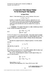
h where the elements are called control or squares. We also have given a dual mesh Th∗ = {Vk }k=1 volumes. Figure 1 illustrates a primal and dual mesh made of squares.

Figure 1: Example of regular mesh made of squares and its dual triangulation. Let us consider P h = Qr (Th ) the space of continuous and piecewise polynomials of degree r on 1 each element of the primal mesh, and PDh = P h ∩HD (Ω) (which are the functions in P h that vanish h 0 ∗ in ∂ΩD ). Let M = Q (Th ) be the space of piecewise constant functions on the dual mesh Th∗ . We mention here that our analysis may be extended to different spaces and differential equations. See for instance [31] where we consider GMsFEM spaces instead of piecewise polynomials. The discrete version of (13) is to find ph ∈ PDh and λ ∈ M h such that a(ph , v h ) + a(v h , λh ) = F (v h ) a(ph , µh ) = F (µh )

for all v h ∈ PDh , for all µh ∈ M h .

Let {ϕi } be the standard basis of PDh . We define the matrix Z A = [ai,j ] where aij = Λ∇ϕi · ∇ϕj .

(15)

(16)

Ω

Note that A is the finite element stiffness matrix corresponding to finite element space PDh . Introduce also the matrix Z A = [ak,j ] where aij = −Λ∇ϕj · n. (17) ∂Vk

7

With this notation, the matrix form of the discrete saddle point problem is given by, # "    T f uh A A = h λ f A O

(18)

where the vector f is defined by, f = [fi ]

withfi =

Z

q ϕi

f=

Ω

Nh∗ [f k ]k=1

=

Z

q.

Vk

For instance, in the case of the primal and dual triangulation of Figure 2 and polynomial degree r = 2, the finite element matrix A is a sparse matrix with 19 diagonals. Also, for a control volume Vk that has no empty interception with, there are at most 9 supports of basis functions ϕj , see Figure 2. Then, matrix A is also sparse.

Figure 2: Control volumes that intersect the support of a Q2 basis function. Remark 1. Note that matrix A is related to classical (low order) finite volume matrix. Matrix A is a rectangular matrix with more columns than rows. Several previous works on conservative high-order approximation of second order elliptic problem have been designed by “adding” rows using several constructions. One can proceed as follows: 1. Construct additional control volumes and test the approximation spaces against piecewise constant functions over the total of control volumes (that include the dual grid element plus the additional control volumes). We mention that constructing additional control volumes is not an easy task and might be computationally expensive. We refer the interested reader to [12, 13, 14] for additional details. 8

2. Use as additional the basis functions the basis functions that correspond to nodes other than vertices to obtain an FV/Galerkin formulation. This option has the advantage that no geometrical constructions have to be carried out. On the other hand, this formulation seems difficult to analyze. Also, some preliminary numerical tests suggest that the resulting linear system becomes unstable for higher order approximation spaces (especially for the case of high-contrast multiscale coefficients). 3. Use the Ritz formulation with restrictions (15). Note that if the polynomial degree r = 1, in the linear system (18), the restriction matrix corresponds to the usual finite volume matrix. This matrix is known to be invertible. In this case, the affine space W is a singleton. Moreover, the only function u satisfying the restriction is given by u = (A)−1 b. The Ritz formulation (15) reduces to the classical finite volume method. Then, in the Ritz sense, the solution of (15) is not worse that any of the solutions obtained by the methods 1. or 2. mentioned above. Furthermore, the solution of the associated linear system (15), which is a saddle point linear system can be readily implemented using efficient solvers for the matrix A (or efficient solvers for the classical finite volume matrix A); See for instance [7]. Additionally, we mention that the analysis of the method can be carried out using usual tools for the analysis of restricted minimization of energy functionals and mixed finite element methods. The numerical analysis of our methodology is under current investigation and it will presented elsewhere.

5 Analysis We show next that imposing the conservation in control volumes using Lagrange multipliers does not interfere with the optimality of the approximation in the H 1 norm. As we will see, imposing constraints will result in non optimal L2 approximation but we were able to reformulate the L2 approximation to get back to the optimal approximation by using the discrete Lagrange multiplier as a corrector. Before proceeding we introduce notation to avoid proliferation of constants. We use the notation A  B to indicate that there is a constant C1 such that A ≤ C1 B. If additionally there exist C2 such that B ≤ C2 A we write A ≍ B. R 1 1 1 Denote kvk2a = Ω Λ∇v · ∇v for all v ∈ HD (Ω) and let us remind that Hdiv := {v ∈ HD (Ω) : h h 1 Λ∇v ∈ H(div, Ω)}, and set V = Span{PD , Hdiv }. We present a concrete example of the norms of V h and M h in the next section, see (37) and (38), respectively. Assumption A: There exist norms k · kV h and k · kM h for V h and M h , respectively, such that 1. Augmented norm: kvka ≤ kvkV h forall v ∈ Vh . 2. Continuity: there exists k¯ak ∈ R such that |¯a(v, µh )| ≤ k¯ak kvkV h kµh kM h ∀v ∈ Vh and µh ∈ M h . 9

(19)

3. Inf-Sup: there exists α > 0 such that inf

sup

µh ∈M h vh ∈P h

D

a(v h , µ) ≥ α > 0. kv h ka kµh kM h

(20)

Remark 2. The Inf-Sup condition above can be replaced by: there exists α > 0 such that inf

sup

µh ∈M h vh ∈P h D

a(v h , µ) ≥ α > 0. kv h kV h kµh kM h

(21)

We have the following result. Assume that {p, λ} is the solution of (13) and {ph , λh } the solution of (15). We have the following result. The proof uses classical approximation techniques for saddle point problems. Theorem 3. Assume that “Assumption A” holds. Then, there exists a constant C such that   kak h inf ku − v h kV h . kp − p ka 6 2 1 + h α v ∈PDh Proof. Note that in both problems, (13) and (15), µ belongs to the finite dimensional subspace M h . Also, the exact solution of the Lagrange multiplier component of (14) is λ = 0. Now we derive error estimates following classical saddle point approximation analysis. Define  W h (q) := vh ∈ PDh : a(v h , µ) = F (µ) for all µ ∈ M h and

First we prove

 W h := vh ∈ PDh : a(v h , µ) = 0 for all µ ∈ M h . kp − ph ka ≤ 2

inf

w h ∈W h (q)

kp − w h ka .

(22)

The inf-sup above in (20) implies that W h (q) (as well as W h ) is not empty. Take any w h ∈ W (q) and solve for z h the problem, h

a(v h , z h ) = F (z h ) − a(w h , z h )

for all z h ∈ Wh .

(23)

Since a is elliptic there exists a unique solution and therefore ph = v h − w h ,

10

(24)

where ph is the solution of (15). We have from (14) and (15) and using (23) that a(v h , v h ) = a(ph − w h , v h ) = a(ph , v h ) − a(w h , v h ) = F (v h ) − a(w h , v h ) = a(p, v h ) − a(w h , v h ) = a(p − w h , v h ). Then, by using the elipticity of a, we have kv h k2a = a(v h , v h ) = a(p − w h , v h ) 6 kp − w h ka kv h ka .

(25)

Then kp − ph ka 6 kp − w h ka + kw h − ph ka 6 kp − w h ka + kp − w h ka = 2kp − w h ka so that (22) holds true. We now show that inf

h

w h ∈W h (q)

kp − w ka 6



kak 1+ α



inf kp − v h kV h

h vh ∈PD

(26)

Take any v h ∈ W h . The inf-sup condition (20) implies that there exists a unique z h ∈ PDh such that a(z h , µ) = a(p − v h , µ)

for all µ ∈ M h .

Then we have that z h 6= 0, a(z h , µ) ≥α kz h ka kµkM h and therefore 1 a(z h , µ) 1 a(p − v h , µ) · = · α kµh k α kµkM h 1 6 kakkp − v h kV h . α

kz h ka 6

Note that we have used the continuity of a ¯ in the extended norm k · kV h . Put w h = z h + v h then a(w h , µ) = a(z h , µ) + a(v h , µ) = a(p − v h , µ) + a(v h , µ) = a(p, µ) = F (µ). 11

Therefore we have that w h ∈ Wh (q). Moreover, kp − w h ka 6 kp − v h ka + kv h − w h ka 6 kp − v h ka + kzh ka kak 6 kp − v h ka + kp − v h kV h α   kak 6 1+ kp − v h kV h . α Combining (22) and (26) we get the result. As showed up in the numerical experiments the error kp−ph kL2 (D) is not optimal but according to the next result if we correct ph to ph + λh we do get optimal approximation. The proof of the following results follows a duality argument similar to that of the Aubin-Nitsche method; see [32, 9]. Since we will use regularity theorem, we will assume from now on that Λ = I (identity). In this case, k · ka = | · |1 , and we will show in the next section that “Assumptions A and B” hold and 1/α = O(1) and |¯a| = O(1). Theorem 4. Assume that the problem (14) is regular (see [32]) and “Assumptions A and B” hold. Then, kp − (ph + λh )kL2 (Ω)  hkp − ph ka . Proof. For g ∈ L2 define S1h g and S0h g as the solution of h

a(S1h g, v h)

, S0h g)

+ a(v Z h a(S1 g, µ) = gv h µ

=

Z

gv h

D

1 for all v h ∈ Hdiv

(27)

for all µ ∈ M h .

(28)

D

Analogously, define Sg as the solution of R a(Sg, v) = RD gv a(Sg, µh) = D gµh

1 for all v ∈ Hdiv , h for all µ ∈ M h .

(29)

Observe that ph = S1h q, λh = S0h q and p = Sq. According to our previous result in Theorem 3 combined with standard regularity and approximation results ([32]) we have ||Sg − S1h g||a  inf ||Sg − v h ||V h  h||Sg||H 2(Ω)  h||g||L2(Ω) . h vh ∈PD

(30)

Recall that, kp − (ph + λh )kL2 (Ω) = sup g∈L2

12

(p − (ph + λh ), g) . kgkL2 (Ω)

(31)

By using the definition of S, S0h and S1h in (27) and (29) we get (p − (ph + λh ), g) = (p, g)0 − (ph , g)0 − (λh , g)0   = a(Sg, p) − a(S1h g, ph )0 + a(ph , S0h g) − a(S1h g, λh )   = a(Sg, p) − a(S1h g, ph )0 + a(S1h g, λh ) − a(ph , S0h g) Z  h = a(Sg, p) − f S1 g − a(ph , S0h g) D

= a(Sg, p) − a(p, S1h g) − a(ph , S0h g) = a(p, Sg − S1h g) − a(ph , S0h g)

= a(p − ph , Sg − S1h g) + a(ph , Sg − S1h g) − a(ph , S0h g)   = a(p − ph , Sg − S1h g) + a(ph , Sg) − a(S1h g, ph ) − a(ph , S0h g)  Z Z h h h h = a(p − p , Sg − S1 g) + gp − gp D

=

≤ 

D

h

a(p − p , Sg − S1h g) ||p − ph ||a ||Sg − S1h g||a h|p − ph |a ||g||L2(Ω) .

In the last step we have used (30). Replacing the last inequality in (31) we get our result.

6 The case of piecewise polynomials of degree two in regular meshes In this section we consider a regular mesh made of squares. See Figure 1. Define ∗

∗

Γ∗h

=

Nh [

∂Vk =

i=k

Nh [

(∂Vk ∩ ∂Vk′ )

i=k,k ′ =1

that is, Γ∗h is the interior interface generated by the dual triangulation. For µ ∈ M h define [µ] on Γ∗h as the jump across element interfaces, that is, [µ]|∂Vk ∩∂Vk′ = µk − µk′ . Note that for p ∈ V h ∗

a(p, µ) =

Nh X k=1

µk

Z

−∇p · n =

Z

−∇p · n [µ] .

Γ∗h

∂Vk

For each control volume Vk , denote by E(k) the set of element of the primal mesh that intersect Vk . Note that in each control volume we have Z X Z −∇p · n = −∇p · n. ∂Vk

ℓ∈E(k)

13

∂Vk ∩Rℓ

To motivate the definition of the norms we study the continuity of the bilinear form a. Observe that, !2 ! ! Z Z Z 1 −∇p · n [µ] ≤ h (∇p · n)2 [µ]2 . h ∂Vk ∩∂Vk′ ∂Vk ∩∂Vk′ ∂Vk ∩∂Vk′ And therefore by applying Cauchy inequality and adding up we get, !1/2 !1/2 Z Z 1 [µ]2 . (∇p · n)2 |a(p, µ)| ≤ h h Γ∗h Γ∗h Using an inverse inequality ( [32]) we get that ∗

h

Z

(∇p · n)2 = h

Γ∗h

Nh Z X k=1

(∇p · n)2

Nh∗

=

X X

h

k=1 ℓ∈E(k)

≤C

Z

(∇p · n)2

Nh∗ X X Z

Nh Z X

=C

Z

|∇p|2 + h2 |∆p|2

Vk ∩Rℓ

|∇p|2 + h2 |∆p|2

Rℓ

ℓ=1

(33)

∂Vk ∩Rℓ

k=1 ℓ∈E(k)

=C

(32)

∂Vk

|∇p|2 + h2 Ω

Nh Z X




|∆p|2

Rℓ

ℓ=1




(34)

(35) !

.

(36)

Now we are ready to define the norm kpk2V h

=

|p|2H 1 (Ω)

2

+h

Nh Z X ℓ=1

|∆p|2

(37)

Rℓ

Note that if p ∈ Q1 then kpk2V h = |p|2H 1 (Ω) . Also, if p ∈ Q2 we have kpk2V h ≤ c|p|2H 1 (Ω) by using inverse inequality. Also define the discrete norm for the spaces of Lagrange multipliers as Z 1 2 kµkM h = [µ]2 . (38) h Γ∗h We have shown above that the form a is continuous, that is, there is a constant C such that, |a(p, µ)| ≤ CkpkV h kµkM h . This also implies continuity in the H 1 norm. Now let us show the inf-sup condition. 14

Theorem 5. Consider the norms for k · ka = | · |H 1 (Ω) and M h defined in (38), respectively. There is a constant α such that, a(v h , µ) ≥ α > 0. (39) inf sup µ∈M h vh ∈Q1 kv h ka kµkM h Proof. Given µ ∈ M h define v ∈ Q1 as v(xi ) = µ(xi ) if xi is a vertex of the primal mesh in Vi and v(xi ) = 0 if xi is a vertex of the primal mesh on ∂ΩD . We first verify that, |v|2H 1 = kvk2V h ≍ kµk2M h .

(40)

ˆ = [0, 1] × [0, 1]. It is enough to verify this equivalence of norms in the reference square R Denote by Pi , i = 1, 2, 3, 4 the values of the reference function vˆ at the nodes of the reference element. We have, vˆ = P1 (1 − x)(1 − y) + P2 (x)(1 − y) + P3 (1 − x)y + P4 xy, and we can directly compute ∂x vˆ = (P2 − P1 )(1 − y) + (P4 − P3 )y and ∂y vˆ = (P3 − P1 )(1 − x) + (P4 − P2 )x. Therefore, Z 1 21 (P2 − P1 ) + (P4 − P3 ) ≤ ∂x vˆ2 4 4 ˆ R 1 1 1 = (P2 − P1 )2 + (P4 − P3 ) + (P2 − P1 )(P4 − P3 ) 3 3 6 5 5 ≤ (P2 − P1 ) + (P4 − P3 ) . 12 12 Analogously, 1 (P2 − P1 ) + (P4 − P3 ) ≤ 4 4 21

Z

∂y vˆ2 ≤ (P2 − P1 )

R

5 5 + (P4 − P3 ) . 12 12

This prove (40). Now we verify that Z

Γ∗h

∇v · n[µ]  kµk2M h .

Observe that if R is an element of the primal triangulation, Γ∗h ∩ R can be written as the union of four segments denoted by Γ∗i,R where i = 4(up), 2(lef t), 3(right), 1(down). Working again on the reference square, we have Z

ˆ∗ Γ

ˆ 1,R

∇ˆ v · n[P2 − P1 ] = P2 − P1

Z

1/2

(P2 − P1 )(1 − y) + (P4 − P3 )y

0

1 3 = (P2 − P1 )2 + (P2 − P1 )(P4 − P3 ) . 8 4 15

Analogously, Z Z Z

ˆ∗ Γ

1 3 ∇ˆ v · n[P4 − P3 ] = (P4 − P3 )2 + (P2 − P1 )(P4 − P3 ) 8 4 ˆ

ˆ∗ Γ

1 3 ∇ˆ v · n[P3 − P1 ] = (P3 − P1 )2 + (P3 − P1 )(P4 − P2 ) 8 4 ˆ

ˆ∗ Γ

3 1 ∇ˆ v · n[P4 − P2 ] = (P4 − P2 )2 + (P3 − P1 )(P4 − P2 ) 8 4 ˆ

2,R

3,R

4,R

If we add these last form equations we get Z ∇v · n[µ]  (P2 − P1 )2 + (P3 − P1 )2 + (P4 − P2 )2 + (P4 − P3 )2 . Γ∗h ∩R

This finish our proof. Assumption B: Let v ∈ H 2 (Ω). Then following approximation holds inf kv − vh kV h ≤ Ch|v|H 2 (Ω) .

h vh ∈PD

We mention that, for regular meshes and Q2 finite element spaces and the norm k · k defined in (37), Assumption B follows from classical finite element approximation and stability results of finite element interpolation operators. See [32]. Corollary 1. Consider the norms for V h and M h defined in (37) and (38), respectively. If p ∈ H 2 (Ω) and “Assumptions A and B” hold, then kp − ph ka  inf ku − v h kV h  h|p|H 2 (Ω) vh ∈Q2

and if the problem is regular kp − (ph + λh )k0  hkp − ph kV h  h2 |p|H 2 (Ω) . We finish this section by mentioning that our analysis is valid for high order finite element on regular meshes made of triangles since a similar analysis holds in this case.

7 Numerical Experiments We consider the Dirichlet problem (1) and employ the meshes depicted in Figure 1 with a variety of mesh sizes. We impose conservation of mass as described in the paper by using Lagrange multipliers. For this paper, we solved the saddle point linear system by LU decomposition. Several iterative solvers can be proposed for this saddle point problem but this will be considered in future 16 studies and not here.

7.1 Regular case with Dirichlet’s boundary condition Consider Ω = [0, 1] × [0, 1]. We consider a regular mesh made of 2M × 2M squares. The dual mesh is constructed by joining the centers of the elements of the primal mesh. We performed a series of numerical experiments to compare properties of FEM solutions with the solution of our high order FV formulation (to which we refer from now on as FV solution). The FV formulation with correction we denote by FV + λ.

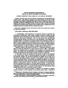
7.2 Smooth problem with Dirichlet boundary conditions We selected the following forcing term and exact solution, q(x, y) = 2π(cos(πx) sin(πy) − 3 sin(πx) cos(πy) + π sin(πx) sin(πy)(−x + 3y)), p(x, y) = sin(πx) sin(πy)(−x + 3y). First we implemented the case of Q1 elements that corresponds to the classical finite element and classical finite volume methods. We compute L2 and H 1 errors. We present the results in Table 0 10 1 and displayed graphically in Figures 3 and 4. We observe here optimal convergence of both FEM (2.0104) strategies. FV (2.0109) FV+λ (2.0303) 10-2

10-4

10-6 -3 10

10-2

10-1

100

Figure 3: Log-log graphic of FEM and FV L2 errors for numerical solutions of Example 1, using Q1 discretization, h = 2−M , M = 1, . . . , 9. We now consider the case of Q2 finite element space. We have computed the FEM solution as well as the solution of the saddle point system (15). We call this last solution the High order FV solution. We estimate the L2 and H 1 errors for both FEM and FV and compare the results through the log-log graphics shown in Figure 5 and Figure 6. See also the Table 2 for comparisons. Numerical convergence is observed with a rate of 2 for the H 1 error. The error p − ph is not optimal in L2 . For this error, the observed convergence rate is close to 2 but if we observe the error p − (ph + λh ) in L2 we estimate a convergence rate of 3. These results coincide with our theoretical predictions four our High order FV formulation.

17

101 FV (1.0078) FEM (1.0084)

100 10-1 10-2 10-3 -3 10

10-2

10-1

100

Figure 4: Log-log graphic of FEM and FV H 1 errors for numerical solutions of Example 1, using Q1 discretization, h = 2−M , M = 1, . . . , 9. We now turn our attention to the norm k · kV h , defined in (37), of the computed error. We introduce the seminorm, Nh Z X 2 |∆p|2 . (41) |p|V h = ℓ=1

Rℓ

Note that kpk2V h = |p|2H 1 + h2 |p|2V h . We present the results in Table 3. We see from this results that the error in the seminorm | · |2V h decays linearly and recall that this seminorm is scaled by a factor h in the definition of the extended norm k · k2V h in (37). Using our high order formulation we compute the conservative approximation of the pressure and a Lagrange multiplier which is used to correct the solution for a improved L2 approximation. Note that the exact solution value of the Lagrange multiplier is λ = 0. We now compute the error in the Lagrange multiplier approximation. The results are presented in Table 4. We observe a convergence of order 2 in the approximation of the Lagrange multiplier. To finish this subsection we compute energy and conservation of mass indicators in Table 5. The energy is defined as Z Z 1 2 E(p) = |∇p| dx − qp (42) 2 Ω Ω while the conservation of mass indicator is given by, J(p) =

X Z R

−∇p · n −

∂R

Z

R

18

q

2 !1/2

.

(43)

M 1 2 3 4 5 6 7 8 9

F EM, L2 Error 1.5538 × 10−1 3.6342 × 10−2 8.9720 × 10−3 2.2548 × 10−3 5.5513 × 10−4 1.3875 × 10−4 3.4685 × 10−5 8.6711 × 10−6 2.1678 × 10−6

F V + λ, L2 Error 1.5103 × 10−1 3.1881 × 10−2 7.5.276 × 10−3 1.9348 × 10−3 4.6095 × 10−4 1.1513 × 10−4 2.8776 × 10−5 7.1935 × 10−6 1.7983 × 10−6

F EM, H 1 Error 1.1297 × 100 5.3226 × 10−1 2.6374 × 10−1 1.3163 × 10−1 6.5833 × 10−2 3.2948 × 10−2 1.6418 × 10−2 8.2838 × 10−3 4.1639 × 10−3

F V, H 1 Error 1.1338 × 100 5.3416 × 10−1 2.6403 × 10−1 1.3172 × 10−1 6.5840 × 10−2 3.2924 × 10−2 1.6489 × 10−2 8.2141 × 10−3 4.1857 × 10−3

Table 1: Table of FEM and FV L2 and H 1 errors for numerical solutions of Example 1, using Q1 discretization, calculated over 9 different values of mesh norm, h = 2−M . M 1 2 3 4 5 6 7 8 9

F EM L2 Error 1.4061 × 10−2 2.1217 × 10−3 2.6860 × 10−4 3.3875 × 10−5 4.2437 × 10−6 5.3075 × 10−7 6.6353 × 10−8 8.2944 × 10−9 1.0369 × 10−9

F V + λ, L2 Error 2.5448 × 10−2 4.9023 × 10−3 6.4789 × 10−4 8.1756 × 10−5 1.0242 × 10−5 1.2810 × 10−6 1.6015 × 10−7 2.0019 × 10−8 2.5024 × 10−9

F EM H 1 Error 1.9302 × 10−1 5.4862 × 10−2 1.4072 × 10−2 3.5418 × 10−3 8.3539 × 10−4 2.2016 × 10−4 5.5043 × 10−5 1.3761 × 10−5 3.4403 × 10−6

F V, H 1 Error 2.2436 × 10−1 7.2895 × 10−2 1.8847 × 10−2 4.7552 × 10−3 1.2667 × 10−3 2.9616 × 10−4 7.4046 × 10−5 1.8512 × 10−5 4.6280 × 10−6

Table 2: Table of FEM and FV L2 and H 1 errors for numerical solutions of Example 1, using Q2 discretization, calculated over 9 different values of mesh norm, h = 2−M .

7.3 Problems with Neumann boundary condition For comparison, we also solve two problems with Neumann boundary conditions. The first problem has a singular forcing term in the form of a font located at (0, 0) and a source located in (1, 1). The computed solution for this problem is shown in the Figure 7. The second problem has a smooth forcing term. 7.3.1 Singular forcing Table 6 shows F EM and F V computed order of convergence of the error. Apart from computing L1 and L2 norms of the error we also include the measure of the error in the seminorm W 1,1 (note that in this case the solution of this problems in not regular and is not in H 1 (Ω)). We observe here that, in terms of approximation, the performance of both strategies FEM and FV perform similarly

19

100 FEM (2.975) FV+λ (2.9467) FV (1.9582)

10-5

10-10 -3 10

10-2

10-1

100

Figure 5: Log-log graphic of FEM and FV L2 errors for numerical solutions of Example 1, using Q2 discretization, h = 2−M , M = 1, . . . , 9. with respect to the order of the polynomials. The main difference between the two computed solution is only the conservation of mass that is being satisfied only by the FV solution. 7.3.2 Smooth forcing To finish our comparison with Neumann boundary condition we consider the case where the flux term is given by q(x, y) = x − y. In Table 7 we show the results. We obtain expected results with our FV formulation being as accurate as the FEM formulation and still satisfying the conservation of mass restrictions.

8 Conclusions and perspectives As we previously announced, we have emphasized the challenges in the construction of new methodologies into a reservoir simulation should have into account the following issues: 1) local mass conservation properties, 2) stable-fast solver and 3) the flexibility of re-use of the novel technique into more complex models (such as to nonlinear time-dependent transport equations equation for the convection dominated transport equation). For Darcy-like model problems with very high contrasts in heterogeneity, the discretization of model (1) alone may be very hard to solve numerically due to a large condition number of the arising stiffness matrix. Moreover, the situation in even more intricate for modeling non trivial two- [19, 25] and three-phase [2, 1] transport convection dominated phenomena problems for flow through porous media (see also other relevant works [27, 4, 17, 5]). In addition, existence, uniqueness and regularity issues for such problems at a fine level out of reach. Thus, numerical simulation of fluid dynamics provide insight into the numerical simulation of fluid flow linked to theory, numerics and applications. 20

100 FV (1.9676) FEM (1.9827) -2

10

10-4

10-6 -3 10

10-2

10-1

100

Figure 6: Log-log graphic of FEM and FV H 1 errors for numerical solutions of Example 1, using Q2 discretization, h = 2−M , M = 1, . . . , 9. With this in mind, as a future perspective is to plug our novel high-order conservative finite element method in a numerical simulator. For the purpose of such study it is necessary to describe a coupled pressure-velocity (elliptic) and convection dominated transport (parabolic with a strong hyperbolic character) conservative solution and stable-fast algorithm to model essentially the interface capturing problems for multiphase flows where neither of the phases can be regarded as dominant. While the volume fractions (or saturation) are gained by solving the pertinent transport equations, fluid flow velocity is solved by solving the Darcy pressure problem; although the need of the pressure as primary unknown, is just the Darcy velocity that we need to plug into the convection dominated transport system. Thus, to achieve a sufficiently coupling between the volume fractions (or saturation) and the pressure-velocity, the full problem can be treated along with a fractional-step numerical procedure [2, 1]; we point out that we are aware about the very delicate issues linked to the discontinuous capillary-pressure (see [3] and the references therein); such issues must be considered no matter how is the time discretization of the convection dominated transport, namely, explicitly or implicitly. Before continuing, remember that Figure 1 illustrates a primal Th and dual Th∗ mesh made of squares. Thus, a feasible time marching algorithm (see, e.g. [2, 1, 19, 25]) to the full set of nonlinear differential model saturation-pressure-velocity equations is given by solving for the saturation, in hyperbolic -parabolic sub-steps, and the total Darcy velocity, in the velocity-pressure sub-steps. The approximation of elliptic pressure equation will take advantage of our high-order conservative finite element method while the transport equation can be handle by fast-accurate finite-volume method, by combining primal and dual meshes as we are using here. Indeed, the fluxes (Darcy velocities) are smooth at the vertices of the cell defining the integration volume in the dual triangularization, since these vertices are located at the centers of non-staggered cells, away from the jump discontinuities along the edges. This facilitates the con21

M 1 2 3 4 5 6 7 8 9

|p − ph |2V h 2.9810 × 100 1.6915 × 100 8.6654 × 10−1 4.3578 × 10−1 2.1820 × 10−1 1.0914 × 10−1 5.4574 × 10−2 2.7288 × 10−2 1.3644 × 10−2

Table 3: Table of scaled seminorm errors, see (41), for FV solution, h = 2−M . Recall that the seminorm | · |2V h in (41) is scaled by a factor h in the definition of the extended norm (37) . M 1 2 3 4 5 6 7 8 9

Error 2.4825 × 10−1 9.9023 × 10−2 2.5293 × 10−2 6.3369 × 10−3 1.5848 × 10−3 3.9623 × 10−4 9.9061 × 10−5 2.4765 × 10−5 6.1913 × 10−5

Table 4: Table of error values for the Lagrange multiplier approximation. struction of second-order and high-order approximations linked to the hyperbolic-parabolic model problem. This also means that the pertinent spatial integrals can be approximated in a straightforward manner. For instance, the finite volume differencing [2, 1, 19], unlike upwind differencing, bypasses the need for Riemann solvers, yielding simplicity, avoiding dimensional splitting in multidimensional problems. In particular, such framework also allows for the extension of the scheme to hyperbolic systems by component-wise application of the scalar framework (for more details see [2, 1, 19] and the references cited therein). Moreover, at the same vertices of the integration volume, the novel high-order conservative finite element method gives the best accurate velocity field even in the presence of highly variable permeability fields, providing useful insights into the numerical simulation of fluid flow. This gives some of the benefits of staggering between primal and dual mesh triangulation by combining our novel high-order conservative finite element method with finite volume for hyperbolic-parabolic conservation laws modeling fluid flow in oil reservoirs and groundwater modeling as well as associated hazards of contamination and transport by ground 22

M 1 M 1

Q1 , E(uF EM ) -4.5230278474 Q1 , J(uF EM ) 5.2434 × 10−6

Q2 , E(uF EM ) -4.523568683883 Q2 , J(uF EM ) 8.2205 × 10−8

Q1 , E(uF V ) -4.5230278425 Q1 , J(uF V ) 2.2928 × 10−14

Q2 , E(uF V ) -4.5233568683864 Q2 , J(uF V ) 1.0261 × 10−13

Table 5: Energy minimization and conservation indicator with h = 2−9 .

Figure 7: Plot of numerical solution for the problem with homogeneous Neumann boundary conditions and singular right hand side. water, CO2 geological sequestration and storage, acid mine drainage remediation, just to name a few up to date subsurface hydrology and groundwater modeling, and geothermal energy associated to petroleum science and engineering. Acknowledgements: E. Abreu (P.I.) thanks financial support FAPESP through grants No. 2014/032049 and CNPq through grants No. MCTI/CNPQ/Universal 445758/2014-7. Ciro Diaz thanks CAPES for a graduate fellowship. Marcus Sarkis thanks in part by nsf-mri 1337943 and nsf-mps 1522663

References [1] E. Abreu, Numerical modelling of three-phase immiscible flow in heterogeneous porous media with gravitational effects, Mathematics and Computers in Simulation, 97 (2014) 234-259. [2] E. Abreu, J. Douglas, Jr., F. Furtado, D. Marchesin and F. Pereira, Three-phase immiscible displacement in heterogeneous petroleum reservoirs. Math. Comput. Simul. 73(1), 2-20 (2006). [3] B. Andreianov and C. Cancs, Vanishing capillarity solutions of Buckley-Leverett equation with gravity in two-rocks medium, Computational Geosciences 17 (3) (2013) 551-572. [4] P. Bastian, A fully-coupled discontinuous Galerkin method for two-phase flow in porous media with discontinuous capillary pressure. Comput. Geosci. 18 (2014) 779-796. 23

L1 L2 W 1,1

Q1 1.8463 1.0000 0.8694

Q2 1.8707 1.0121 0.9983

L1 L2 W 1,1

1.8490 1.0000 0.8590

1.8715 1.0000 0.9977

F EM

FV FV + λ FV + λ

Table 6: Values of L1 , L2 and W 1,1 error order of F EM and F V for the homogeneous Neumann boundary condition problem with singular forcing. L1 L2 W 1,1

Q1 1.9999 1.9999 1.0000

Q2 3.0000 3.0000 2.0000

L1 L2 W 1,1

2.0000 1.9999 1.0000

3.0000 3.0000 2.0000

F EM

FV FV + λ FV + λ

Table 7: Values of L1 , L2 and W 1,1 error order of F EM and F V for the homogeneous Neumann boundary condition problem with smooth forcing. [5] J. Bear and C. Alexander H.-D. Cheng, Theory and Applications of Transport in Porous Media - Modeling Groundwater Flow and Contaminant Transport, 23 Springer Science Business Media B.V. 2010. [6] L. Beiro da Veiga, F. Brezzi, L. D. Marini and A. Russo, Virtual Element Method for general second-order elliptic problems on polygonal meshes, Math. Models Methods Appl. Sci. 26, 729 (2016). [7] M. Benzi, G. H. Golub and J. Liesen, Numerical solution of saddle point problems, Acta numerica 14 (2005) 1-137. [8] D. Boffi, F. Brezzi and M. Fortin, Mixed Finite Element Methods and Applications Vol 44 (Springer Series in Computational Mathematics), Springer Berlin Heidelberg, 2013, 685 pages. [9] D. Braess, Finite elements (III edition) (Theory, fast solvers, and applications in elasticity theory, Translated from the German by Larry L. Schumaker), Cambridge University Press, Cambridge 2007. 24

[10] H. Brezis and F. Analysis, Sobolev Spaces and Partial Differential Equations, Springer Science Business Media, 2010, 600 pages. [11] F. Brezzi, T. J. R. Hughes, L. D. Marini, and A. Masud, A stabilized mixed discontinuous Galerkin method for Darcy flow, Comput. Methods Appl. Mech. Engrg. 195 (2006) 33473381. [12] L. Chen, A New Class of High Order Finite Volume Methods for Second Order Elliptic Equations, SIAM J. Numer. Anal., 47(6) (2010) 4021-4043. [13] Z. Chen, J. Wu and Y. Xu, Higher-order finite volume methods for elliptic boundary value problems, 37(2) (2012) 191-253. [14] Z. Chen, Y. Xu and Y. Zhang, A construction of higher-order finite volume methods, Math. Comp. 84 (2015) 599-628. [15] M. A. Christie and M. J. Blunt, Tenth SPE comparative solution project: a comparison of upscaling techniques. SPE Reserv Eval Eng 4 (2001) 308-317. [16] D. Cortinovis and P. Jenny, Iterative Galerkin-enriched multiscale finite-volume method, Journal of Computational Physics, 277(15) (2014) 248-267. [17] J. Dong and B. Riviere, A semi-implicit method for incompressible three-phase flow in porous media, Comput Geosci (DOI 10.1007/s10596-016-9583-2; First Online: 12 August 2016 ) [18] J. Douglas Jr., F. Furtado and F. Pereira, On the numerical simulation of waterflooding of heterogeneous petroleum reservoirs, Computational Geosciences 1 (1997) 155-190. [19] L. J. Durlofsky, A Triangle Based Mixed Finite Element-Finite Volume Technique for Modeling Two Phase Flow through Porous Media, Journal of Computational Physics 105(2) (1993) 252-266. [20] Y. Efendiev and T. Y. Hou, Multiscale Finite Element Methods: Theory and Applications (Surveys and Tutorials in the Applied Mathematical Sciences) vol. 4 (2009) 234 Pages. [21] Y. Efendiev, J. Galvis, T. Hou, Generalized multiscale finite element methods, Journal of Computational Physics 251 (2013) 116–135. [22] Y. Efendiev, J. Galvis, X. H. Wu, Multiscale finite element methods for high-contrast problems using local spectral basis functions, Journal of Computational Physics 230 (4) (2011) 937–955. [23] J. Galvis, Y. Efendiev, Domain decomposition preconditioners for multiscale flows in high contrast media, SIAM J. Multiscale Modeling and Simulation 8 (2010) 1461–1483.

25

[24] J. Galvis, Y. Efendiev, Domain decomposition preconditioners for multiscale flows in high contrast media. reduced dimension coarse spaces, SIAM J. Multiscale Modeling and Simulation 8 (2010) 1621–1644. [25] M. G. Gerritsen and L. J. Durlofsky, Modeling fluid flow in oil reservoirs, Annu. Rev. Fluid Mech. 37 (2005) 211-38. [26] D. Gilbarg and N. S. Trudinger, Elliptic Partial Differential Equations of Second Order (Classics in Mathematics) Springer, 2015, 518 pages. [27] M. Ghasemi, Y. Yang, E. Gildin, Y. Efendiev and V. Calo, Fast multiscale reservoir simulations using POD-DEIM model reduction. Paper 173271-MS presented at the SPE Reservoir Simulation Symposium, Houston, USA, 22-25 February 2015. [28] G. M. Homsy, Viscous Fingering in Porous Media, Annual Review of Fluid Mechanics, 19 (1987) 271-311. [29] T. J. R. Hughes, A. Masud and J. Wan, A stabilized mixed discontinuous Galerkin method for Darcy flow, Comput. Methods Appl. Mech. Engrg. 195 (2006) 3347-3381. [30] J. D. Jansen and L. J. Durlofsky, Use of reduced-order models in well control optimization, Optimization and Engineering (First Online: 22 February 2016; DOI: 10.1007/s11081-0169313-6) [31] M. Presho and J. Galvis, A mass conservative Generalized Multiscale Finite Element Method applied to two-phase flow in heterogeneous porous media, Journal of Computational and Applied Mathematics, 296 (2016) 376-388. [32] Susanne C. Brenner and L. Ridgway Scott, The mathematical theory of finite element methods (Texts in Applied Mathematics) 15 3rd ed. Springer, New York 2008.

26