Studies in Nonlinear Dynamics and Econometrics Quarterly Journal April 2001, Volume 5, Number 1 The MIT Press
Studies in Nonlinear Dynamics and Econometrics (E-ISSN 1081-1826) is a quarterly journal published electronically on the Internet by The MIT Press, Cambridge, Massachusetts, 02142-1407. Subscriptions and address changes should be addressed to MIT Press Journals, Five Cambridge Center, Cambridge, MA 02142-1407; (617)253-2889; e-mail:
[email protected]. Subscription rates are: Individuals $40.00, Institutions $135.00. Canadians add additional 7% GST. Submit all claims to:
[email protected]. Prices subject to change without notice. Permission to photocopy articles for internal or personal use, or the internal or personal use of specific clients, is granted by the copyright owner for users registered with the Copyright Clearance Center (CCC) Transactional Reporting Service, provided that the per-copy fee of $10.00 per article is paid directly to the CCC, 222 Rosewood Drive, Danvers, MA 01923. The fee code for users of the Transactional Reporting Service is 1081-1826/01 $10.00. For those organizations that have been granted a photocopy license with CCC, a separate system of payment has been arranged. Address all other inquiries to the Subsidiary Rights Manager, MIT Press Journals, Five Cambridge Center, Cambridge, MA 02142-1407; (617)253-2864; e-mail:
[email protected].
c 2001 by the Massachusetts Institute of Technology °
On Impossibility of Limit Cycles in Certain Two-Dimensional Continuous-Time Growth Models Sergey Slobodyan CERGE-EI Prague, Czech Republic
[email protected]
Abstract. This article proves that periodic trajectories are generically impossible in a class of continuous-time growth models that allow a locally indeterminate steady state. Those models reducible to the two-dimensional Lotka-Volterra system of equations constitute the class considered here. Knowledge of the presence or absence of the limit cycles allows a global phase diagram of the system to be constructed. In particular, an explosive steady state implies that all perfect-foresight trajectories diverge to infinity and that the model cannot be used even locally.
Keywords.
indeterminacy, limit cycles
Acknowledgments. For helpful comments we thank William Barnett, Gaetano Antinolfi, James Bullard, John Duffy, Heinz Schaettler, participants in the Computing in Economics and Finance conference in Boston, Massachusetts, and the Eighth Annual Symposium of the Society of Nonlinear Dynamics and Econometrics in Atlanta, Georgia. 1 Introduction
Recently, a number of continuous-time growth models allowing indeterminacy of a steady state for some parameter values have appeared (for a recent review, see Benhabib and Farmer 1999). In two dimensions, local dynamics around a steady state can be saddle path stable (one negative eigenvalue and one positive), stable (two eigenvalues with negative real parts), and absolutely unstable (two eigenvalues with positive real parts). Configurations with one or both eigenvalues being zero or having zero real parts are not generic. One of the necessary conditions for the Hopf bifurcation theorem is two eigenvalues passing through the imaginary axis as some system parameter is varied (see Guckenheimer and Holmes 1997, 151). Therefore, it is widely assumed that when a particular steady state can be both stable and absolutely unstable for different parameter values, the Hopf bifurcation and limit cycles can occur. For example, note 6 in Benhabib and Farmer 1994 states that it is impossible to rule out limit cycles for an absolutely unstable case. This note will prove that for a particular class of two-dimensional growth models, stable or unstable limit cycles are generically impossible even though eigenvalues can pass through the imaginary axis. The question of the existence of limit cycles is very relevant for models that can have an explosive or indeterminate steady state. Two scenarios are generally possible in a Hopf bifurcation. In one, the stable steady state loses stability, becoming absolutely unstable, and a stable limit cycle forms around it. In the other, an unstable limit cycle exists around the stable steady state and disappears when the steady state becomes
c 2001 by the Massachusetts Institute of Technology °
Studies in Nonlinear Dynamics and Econometrics, April 2001, 5(1): 33–40
absolutely unstable. Consider an unstable (explosive) steady state. If a stable limit cycle around it exists, then for the state variable (say, capital) in some neighborhood of the steady state value, one can find an interval of the control variable (say, consumption) values such that the resulting trajectory converges to the limit cycle. The equilibrium dynamics is indeterminate and cyclical, but it stays finite. On the other hand, if no stable limit cycle appears around the unstable steady state, then any perfect-foresight equilibrium trajectory potentially diverges to infinity if initial capital is not equal to the steady-state value. Turning our attention to the stable (indeterminate) steady state, we see that if an unstable limit cycle exists around it, then the dynamics converges to the steady state only for the values of capital close to the steady-state value. Other initial values probably lead to trajectories diverging to infinity. Absence of an unstable limit cycle might mean global stability of the indeterminate steady state. The schemes considered in the previous paragraph demonstrate the importance of knowledge of the presence or absence of the limit cycles for global dynamic analysis of economic models described by two-dimensional systems of differential equations. The model that makes sense locally can completely break down if initial conditions are far from the steady state. There might be no bounded perfect-foresight trajectory converging to an attractor. Limit cycles become especially important for models that allow indeterminate or explosive steady states. The class of models discussed here includes the model described in Benhabib and Farmer 1994 and different modifications of it. The original model is a continuous-time optimal-growth model with endogenous labor and a production function that has constant private returns to scale but increasing social returns to scale because of externalities. For some calibrations, the steady state of the model is indeterminate, whereas for others, it is absolutely unstable. Modifications of the model include Wen 1998, which introduces variable capital utilization with a depreciation rate depending on the utilization rate; Schmitt-Grohe and Uribe 1997, which considers income taxes; and Guo 1999 and Guo and Lansing 1998, which study separate progressive taxes on interest and wage income. As the basis for discussion we will use a slightly modified version of Guo 1999. Section 2 briefly describes the model. Section 3 discusses steady states and their stability. The main result of the paper is presented in Section 4, which also includes an analysis of the global behavior of the model, and Section 5 concludes. 2 The Model
There is a continuum of identical households maximizing the utility ¶ Z ∞µ N 1−χ e −ρt dt, A > 0 log C − A 1−χ 0
(2.1)
where C and N are household consumption and working hours. Households own capital that is rented to firms, and the budget constraint is given by ·
K = (1 − τk )(r − δ)K + (1 − τn )wN − C , K (0) given
(2.2)
with r being the interest rate, w the wage rate, and K the household’s capital stock. Tax rates are given by the following expressions: µ ¶φk Yk , ηk ∈ [0, 1], φk ∈ [0, 1) (2.3a) τ k = 1 − ηk Yk µ ¶φn Yn , ηn ∈ [0, 1], φn ∈ [0, 1) (2.3b) τ n = 1 − ηn Yn where Yn = wN and Yk = (r − δ)K are the household’s taxable labor and interest income. The tax code includes depreciation allowance. Parameters φi and ηi , i ∈ {k, n}, determine the slope and the level of taxes.
34
Impossibility of Limit Cycles
φ 6= 0 means a “progressive” tax, because in this case the marginal tax rate is higher than the average. In a departure from Guo 1999, in which Y k and Y n were the steady state values of the taxable interest and wage income, in this paper they will represent economy-wide averages of respective incomes. This difference means that in a symmetric equilibrium in which every household has the same amount of capital and supplies the same number of hours, tax rates will not depend on the current average output. In Guo 1999, the symmetric equilibrium average tax rates were decreasing in the average level of output, thus generating countercyclical government spending. In the variant used here, the average tax rate in the symmetric equilibrium does not depend on the business cycle stage, which more closely resembles reality. There is also a continuum of identical firms with the production function Y = K aN bK
α−a
N
β−b
(2.4)
where a + b = 1, α > a, β > b, and K and N are economy-wide averages of K and N per firm, which are taken as given by every individual firm. From the profit maximization, the interest rate and the wage rate are given by wN = bY
(2.5)
r K = aY
The government balances its budget at every point in time. Therefore, there is no government debt in the model. In a symmetric perfect-foresight equilibrium, every household has the same amount of capital and supplies the same number of hours, and every firm employs the same quantity of capital and labor. Write the following current-value Hamiltonian as # " µ ¶φ µ ¶φn Yk k Yn N 1−χ (r − δ)K + ηn wN − C (2.6) + µ ηk H = log C − A 1−χ Yk Yn Taking corresponding derivatives, one gets the necessary conditions: 1 = µ C AN
−χ
= (1 − φn )µηn
(2.7a) µ
Yn Yn
·
µ = µρ − µ(1 − φk )ηk lim e −ρt
t→∞
¶φn (2.7b)
w µ
Yk Yk
¶φk (r − δ)
(2.7c)
K = 0 C
(2.7d)
together with the capital accumulation equation ·
K = ηk (r − δ)K + ηn wN − C , K (0) given
(2.8)
Substituting (2.7a) into (2.7b) and (2.7c), recalling that by definition in the symmetric equilibrium Y n = Yn = wN , Y k = Yk = (r − δ)K , and substituting (2.5), we obtain the following set of equations: AC N 1−χ = (1 − φn )ηn bY
(2.9a)
·
aY − δK C = (1 − φk )ηk −ρ C K
(2.9b)
·
Y C aY − δK K = ηk + ηn b − K K K K
(2.9c)
Sergey Slobodyan
35
Y = K αN β K = 0 lim e −ρt t→∞ C
(2.9d) (2.9e)
Switching to logs, c = log(C ), k = log(K ), and y = log(Y ), and using (2.9a) and (2.9d) to obtain y as a function of c and k, we arrive at the following two-dimensional system of differential equations: ·
c = (1 − φk )ηk (a exp(w + uc − vk) − δ − ρ) ·
k = (aηk + bηn ) exp(w + uc − vk) − ηk δ − exp(c − k)
(2.10)
where w =
β (log(A) − log(ηn (1 − φn )) − log(b)) β +χ −1
v =
β − (1 − α)(1 − χ) β +χ −1
u =
β β +χ −1
(2.11)
Finally, changing the coordinates to x = exp(w − vk + uc) y = exp(c − k)
(2.12)
we get the system of equations presented below: ·
x = x{[au(1 − φk )ηk − v(aηk + bηn )]x + vy − uρ − [u(1 − φk ) − v]ηk δ} ·
y = y{[a(1 − φk )ηk − (aηk + bηn )]x + y + φk ηk δ − ρ}
(2.13)
By construction, x and y are non-negative; therefore, only the first quadrant of the (x, y) space should be considered. To simplify notation we will assume in the following that ηk = ηn = η and φk = φn = φ. The main result of the paper, namely, the absense of limit cycles, is not sensitive to this assumption. Note that in the case φ = 0 (flat tax) and η = 1 (tax rate is zero in equilibrium), the system in Equation (2.13) transforms into the model described in Benhabib and Farmer 1994. It is possible to characterize completely the global dynamics of Equation (2.13). We will construct its phase portrait in the indeterminate or explosive case in the following sections. 3 Steady States and Stability
The positive steady state of Equation (2.13) is A = (x ∗ , y ∗ ) = ( ρ−δφη+δη , ρ−δφη+δη(1−a(1−φ)) ). In the remainder of (1−φ)aη (1−φ)a the paper we assume that ρ − δφη > 0, and thus A lies in the first quadrant of the plane. Linearization of Equation (2.13) around this steady state produces " # x ∗ η(au(1 − φ) − v) x ∗ v ∗ J = y∗ y ∗ η(a(1 − φ) − 1) The necessary and sufficient condition for explosive or indeterminate steady state (two stable or unstable roots) is Det|J∗ | = x ∗ y ∗ η(u − v)(1 − φ) > 0. Assuming φ < 1 (progressivity of the tax code not at its topmost level) and η > 0 (symmetric equilibrium tax rate less than 100%), this is equivalent to u − v > 0. Recalling definitions of u and v and simplifying, one gets u−v =
36
Impossibility of Limit Cycles
(1 − α)(1 − χ) >0 β +χ −1
(3.1)
Following Benhabib and Farmer 1994, in which α < 1, χ < 0, Inequality (3.1) becomes β + χ − 1 > 0. This is exactly the celebrated necessary condition for indeterminacy derived in Benhabib and Farmer 1994. Therefore to obtain economically meaningful explosive or indeterminate steady state, we need the following conditions to hold: ρ − δφη > 0 β +χ −1>0
(3.2)
There are other possible steady states of Equation (2.13): B = (0, 0) C = (0, ρ − δφη) ¶ µ uρ + [u(1 − φ) − v]δη ,0 D = au(1 − φ) − v Steady state C lies on the positive half of the y-axis by virtue of Equation (3.2). In the expression for the abscissa of D, the denominator is given by au(1 − φ) − v =
uδφη + [u(1 − φ)δη − v]δη = δη(u − v) > 0
(3.4)
Therefore, D lies in the second quadrant and does not interest us.1 Linearizing Equation (2.13) around the origin, one gets the following Jacobian: " J=
#
−{uρ + [u(1 − φ) − v]δη}
0
0
−(ρ − δφη)
(3.5)
The first nonzero element was estimated in Equation (3.4) and is always negative, whereas the second is negative by Equation (3.2). Therefore, the origin is also stable in Equation (2.13). Finally, for steady state C, one gets " J=
−(u − v)(ρ − δφη + δη)
0
#
η(a(1 − φ) − 1)(ρ − δφη) ρ − δφη
Here the (2,2) element of J is positive, and the (1,1) element is negative if Equation (3.2) holds. Therefore, C is a saddle.
states B and C both represent trajectories diverging to (-∞, −∞) in the (c, k) space, but those trajectories have different asymptotic behavior. Along the trajectory that converges to B, the consumption-to-capital ratio is falling exponentially, but it remains constant for the path converging to C. The change of variables collapses infinity points from the lower half of the (c, k) space onto the vertical half-axis in the (x, y) space. Trajectories with different asymptotic behavior at minus infinity are mapped into different points on the y-axis.
1 Steady
Sergey Slobodyan
37
4 Dulac Criterion and Limit Cycles
The Dulac criterion states that if for the analytic two-dimensional system ·
x = P (x, y) ·
y = Q(x, y)
(4.1)
in a simply connected region G there exists a continuously differentiable function B(x, y), such that ∂(P B) + ∂(QB) does not change sign in G, then there are no simple closed curves in G that are unions of paths ∂x ∂y of the system.2 In particular, there are no limit cycles (see Andronov et al. 1973). Proposition 1. For a system 3 ·
x = x(a1 x + b1 y + c1 ) ·
y = y(a2 x + b2 y + c2 ) the Dulac function is B(x, y) = x k−1 y h−1 , where k =
b2 (a2 −a1 ) , 1
h=
a1 (b1 −b2 ) , 1
(4.2) and 1 = a1 b2 − a2 b1 6= 0. Then
a1 c2 (b1 − b2 ) b2 c1 (a2 − a1 ) k−1 h−1 ∂(P B) ∂(QB) + =( + )x y ∂x ∂y 1 1
(4.3)
B) + ∂(QB) vanishes only along the integral curves x = 0 and When ξ = a1 c2 (b1 − b2 ) + b2 c1 (a2 − a1 ) 6= 0, ∂(P ∂x ∂y y = 0. It does not change sign in the interior of any of the four quadrants. Therefore, system (4.2) does not have limit cycles when ξ 6= 0.
Also, it can be shown that in this case there can be no closed contours that are unions of paths. After some algebraic transformations, it can be shown that the condition on ξ amounts to Tr(J∗ ) = a1 x ∗ + b2 y ∗ 6= 0, where (x ∗ , y ∗ ) denotes the steady state with nonzero x and y, and J∗ is the Jacobian of Equation (4.2) at this steady state. When Tr(J∗ ) = 0, all trajectories of the system are closed orbits. One of the necessary conditions of the Hopf bifurcation theorem is two eigenvalues crossing the imaginary axis with Tr(J∗ ) = 0 for a critical value of some parameter. Further change of the parameter leads to the appearance of a stable or unstable limit cycle around the steady state, with the magnitude depending on the difference between the current and the critical value of the parameter. As follows from Equation (4.3), this scenario is impossible in system (4.2), because closed periodic orbits exist only when Tr(J∗ ) = 0. Not all necessary conditions of the Hopf bifurcation theorem are satisfied in system (4.2), and the Hopf bifurcation is impossible as a result. An obvious and quick calculation assures one that system (2.13) has the same structure as system (4.2). Therefore, limit cycles are impossible in it generically. System (2.13) is obtained as a transformation of Equation (2.10), and therefore we have just proven that closed orbits, in particular limit cycles, are impossible in Guo 1999 except for a unique configuration of parameters when all the system’s trajectories are closed orbits. Absence of limit cycles allows us to construct a global phase portrait of Equation (2.13), which is presented in Figure 1 for the case of indeterminate (stable) steady state. The whole state space is divided into regions of attraction of two steady states, A and B. Any trajectory that starts above the stable manifold of C converges to the positive steady state A. On the other hand, if A becomes explosive, then no trajectory converges to it, and no trajectory remains bounded. All perfect-foresight paths diverge to infinity.4
that Bendixson’s criterion is a special case of Dulac’s with B(x, y) = 1. is a two-dimensional Lotka-Volterra system. Lotka-Volterra systems are studied extensively in mathematical biology. 4 The only trajectory that remains bounded is the one that starts exactly at A. In this paper we do not consider trajectories converging to the origin. 2 Note 3 This
38
Impossibility of Limit Cycles
y = EXP (c − k)
0.2
A
0.15
dx/dt=0
0.1
dy/dt=0
0.05 C 0 0
B 0.05
0.1
0.15
0.2
0.25
0.3
x = EXP (w + u * c − v * k) Figure 1 Phase portrait of the transformed system in (x, y) variables.
It is obvious to check that in a special case φi = 0, ηi = 1, i = k, n, system (2.13) has the same general form as Equation (4.2). Therefore, limit cycles are also impossible there.5 In this case, the tax rates are zero at any level of income, and this is the model described in Benhabib and Farmer 1994. Immediate calculation shows that in the case where interest income is taxed without the depreciation allowance, after the change of variables similar to that in Equation (2.12), the resulting system of differential equations still has the structure of Equation (4.2), and there are no limit cycles. Setting φk = φn = φ, ηk = ηn = η, in a model without depreciation allowance, one arrives at the model described in Schmitt-Grohe and Uribe 1997. Calculations similar to those performed above show that the model described in Wen 1998 also can be reduced to Equation (4.2), therefore proving the absence of limit cycles in that model. In all these models the steady state can be indeterminate or absolutely unstable for some parameter values. 5 Conclusion
In this paper we have shown that in a set of models derived from the one described in Benhabib and Farmer 1994, limit cycles are generically impossible even though a steady state can move from being absolutely stable (locally indeterminate) to absolutely unstable by having two eigenvalues pass the imaginary axis. Such passage is a necessary condition for the presence of the Hopf bifurcation and, consequently, a limit cycle. This class of models can be reduced, however, to a two-dimensional Lotka-Volterra system of differential equations that does not allow limit cycles. Parameter values that lead to an explosive (unstable) steady state are not more “pathological” than those resulting in an indeterminate one. For example, in Benhabib and Farmer 1994, the steady state becomes absolutely unstable if labor externality is as high as in the indeterminate case but capital externality is small or zero. In the case of an absolutely unstable steady state, no perfect-foresight trajectory converges to it, and the
5 For
more detailed study of the global deterministic and stochastic dynamics of this system, see Slobodyan 2001.
Sergey Slobodyan
39
model cannot be used even locally. Full characterization of the global dynamics allows new questions about the model’s behavior to be studied (for an example, see Slobodyan 2001). References Andronov, A. A., E. Leontovich, I. Gordon, and A. Maier. (1973). Qualitative Theory of Second-Order Dynamical Systems. New York: John Wiley & Sons. Benhabib, J., and R. E. Farmer. (1994). “Indeterminacy and increasing returns.” Journal of Economic Theory, 63: 97–112. Benhabib, J., and R. E. Farmer. (1999). “Indeterminacy and sunspots in macroeconomics.” In J. Tailor and M. Woodford (eds.), Handbook of Macroeconomics. Amsterdam: North Holland, pp. 387–448. Guckenheimer, J., and P. Holmes. (1997). Nonlinear Oscillations, Dynamical Systems, and Bifurcations of Vector Fields. New York: Springer. Guo, J.-T. (1999). “Multiple equilibria and progressive taxation of labor income.” Economics Letters, 65: 97–103. Guo, J.-T., and K. J. Lansing. (1998). “Indeterminacy and stabilization policy.” Journal of Economic Theory, 82: 481–490. Schmitt-Grohe, S., and M. Uribe. (1997). “Balanced-budget rules, Distortionary taxes, and aggregate instability.” Journal of Political Economy, 105: 976–1000. Slobodyan, S. (2001). “Sunspot fluctuations: A way out of a development trap?” Working paper no. 175, CERGE-EI, Prague. Wen, Y. (1998). “Capacity utilization under increasing returns to scale.” Journal of Economic Theory, 81: 7–36.
40
Impossibility of Limit Cycles