On Temporal Logic Programming Using Petri Nets - System ...

IEEE TRANSACTIONS ON SYSTEMS, MAN, AND CYBERNETICS—PART A: SYSTEMS AND HUMANS, VOL. 29, NO. 3, MAY 1999

245

On Temporal Logic Programming Using Petri Nets Abbas K. Zaidi, Member, IEEE Abstract— A methodology for modeling temporal (timesensitive) aspects of discrete-event systems is presented. A formalism of temporal logic which incorporates both point and interval descriptions of time is formulated, which is an extension of Allen’s interval logic [1]. A formal axiomatic system of this point-interval logic is presented. A graph model is shown to implement the axiomatic system of point-interval logic. This graph-based approach transforms the system’s specifications given by temporal statements into a graph structure. The graph-based temporal inference engine (TIE) identifies temporal ambiguities and errors (if present) in the system’s specifications, infers new temporal relations among system’s intervals, and identifies the user-defined intervals of interest.

I. INTRODUCTION

T

HE growing need for a formal logic of time for modeling and analyzing real world systems has led to an emergence of various kinds of representations and reasoning schemes for temporal information. The earliest attempts at formalizing a time calculus date back to 1941 by Findlay [2], and 1955 by Prior [3], [4]. Since then, there has been a number of attempts on issues related to this subject matter, like topology of time [5], first-order and modal approaches to time [6]–[18], treatments of time for simulating action and language, etc. Several attempts on mechanizing the temporal reasoning processes have also been reported in the literature [19]–[24]. The list of references provided in this paper is not at all exhaustive and may have missed some of the major contributions; for a comprehensive discussion on issues and an overview of temporal methodologies, the reader is referred to [4]. A majority of these approaches is formulated to handle issues relevant to a specific application area of interest to the scholar(s) who proposed the approach. Therefore, each approach comes with its advantages in addressing certain issues and disadvantages for lack of generality in handling others. Artificial Intelligence, software engineering, planning, cognitive sciences, time-sensitive databases, program verification and modeling of discrete-event systems are some of the examples of the application areas which have contributed mainly to the formulation of time calculi. This paper presents an approach for the modeling and subsequent analysis of the temporal aspects of discreteevent systems. A system’s temporal aspects might be represented in terms of properties that hold for certain time intervals, processes taking some time to complete, and/or events/occurrences requiring virtually no time to take place. In order to model a system’s temporal aspects, one, therefore, Manuscript received June 25, 1997. This work was supported by the Air Force Office of Scientific Research under Contract F49620-95-1-0134 and the Office of Naval Research under Contract N00014-93-1-0912. The author is with the Department of Computer Science, Mohammad Ali Jinnah University, Karachi, Pakistan. Publisher Item Identifier S 1083-4427(99)01453-8.

needs to have a formalism capable of handling both interval and point descriptions of various components of the system. An extension of Allen’s [1], [7]–[11] interval logic that incorporates both descriptions, point and interval, of time is presented. The new formalism, called point-interval temporal logic (PITL), extends the axiomatic system of interval logic by adding new axioms to it. A Petri net model is shown to represent this axiomatic system by transforming the system’s specifications given by temporal statements of pointinterval logic into Petri net structures. A temporal inference engine (TIE) based on this Petri net representation infers new temporal relations among system intervals, identifies temporal ambiguities and errors (if present) in the system’s specifications, and finally identifies the intervals of interest defined by the user. The real strength of this inference engine is that it performs all these functions by completely avoiding the combinatorial nature of the problem inherent in the inference engines of its kind [20]. The paper is organized as follows. Section II presents the definitions of different notions and terms used in the approach together with an introduction of PITL. The section also presents an analytical model for the temporal relations. A transformation of this model to an equivalent Petri net representation is presented in Section III. The structure of Petri net representing temporal relations among intervals is shown to reveal inconsistencies and incompleteness present in the system. The graph-based inference engine, TIE, is also presented in this section. Section IV applies the result of the methodology to an example problem. Finally, Section V concludes the discussion by summarizing the contributions and identifying future extensions of the approach.

II. MATHEMATICAL MODEL Definition 1: Interval: An interval is denoted by a symbol, , where i.e., a letter or a digit, and is defined as . In this definition denotes “start of ” and “end of ”. The two bounds are abstract notions and may not have numerical values assigned to them. The intervals considered in this paper are all closed intervals. Definition 2: Interval Length: The length of an interval , denoted by , is defined as . with is a point Definition 3: Point: An interval is a point interval or point, also denoted interval; . In a system description, a point may be used to signify as an occurrence or an event. Definition 4: Temporal Relation : The temporal relation is a truth functional binary relation defined as

1083–4427/99$10.00  1999 IEEE

246

IEEE TRANSACTIONS ON SYSTEMS, MAN, AND CYBERNETICS—PART A: SYSTEMS AND HUMANS, VOL. 29, NO. 3, MAY 1999

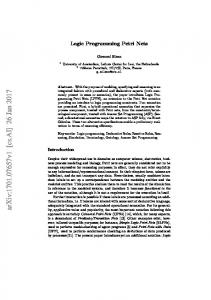
where is the set of intervals and and are the Boolean values, true and false. and Definition 5: Composite Interval: Let be two intervals, where and , then they are jointly represented by a composite interval . By definition or simply . and Definition 6: Composite Point: Let represent a single point on the time line, i.e., , then . the composite point is represented as A. Point-Interval Temporal Logic The point-interval logic presented in this paper is an extension of Allen’s interval logic [1], [7]–[11]. The formalism considers a single time line. Any two intervals with nonzero lengths on this time line are related by one of the seven relationships presented in Fig. 1, case I. This set of seven temporal relations between two intervals was first presented by Allen [1]–[3] in his interval logic. The underlying assumption of the interval logic is the nonzero lengths of time intervals [4]. The present approach relaxes this assumption and allows intervals with zero lengths—points. Case II, Fig. 1, presents two possible temporal relations between two points. Finally, case III, Fig. 1, presents the possible set of temporal relations between a point and an interval. From now on, the term interval is used to refer both intervals and points if not explicitly stated otherwise. represents Definition 7: Set of Temporal Relations, : and is given as the set of temporal relations Before, Meets, Overlaps, Starts, During, Finishes, Equals Proposition 1: The temporal relations presented in Fig. 1 are mutually exclusive and exhaustive, i.e., is an element of , then there does not 1) if in , such that holds true; exist an and there must exist an 2) for any two intervals in such that either or holds true (with the exception of Equals relation where ). B. Analytical Model An analytical representation of temporal relations among intervals is shown in Fig. 1. According to this representation, a temporal relation between two intervals can be described as a set of algebraic inequalities among points representing the start and end of these intervals. and , on a single time line can be related Two points, to each other by one of the following four relations: ; 1) ; 2) ; 3) ? (? represents “unknown”. This is added to 4) incorporate incomplete information.) With these four possibilities and the analytical model of between two intervals and Fig. 1, a temporal relation

Fig. 1. Temporal relations in PITL.

can be represented as a four-digit string made of elements ? , where the first (left-most) from the alphabet and , second digit digit represents the relation between and , third digit represents relation between between and , and fourth between and . The representation does and . not take into account the point or interval nature of The information about the nature of intervals is assumed to be known; however, this four-digit representation can be extended to accommodate this feature as well. (known or unThe description of a temporal relation and , known or partially known) between two intervals therefore, requires only 8 bits (for a computer implementation). This byte representation of a temporal relation between two intervals, and the nature of the intervals (which requires 1 bit for each interval) are all that is required to store (and maintain) complete, or partially/totally incomplete information about the two intervals. Even if one needs to store temporal relations between all possible combinations of intervals from a set of intervals, it will take bytes to store all

ZAIDI: ON TEMPORAL LOGIC PROGRAMMING

247

this information. Temporal inconsistencies can be identified by checking inconsistent patterns of this 8-bit representation. C. Axioms of Point-Interval Logic 1) Point Axioms: , and be points defined on a single time line. Let The following four (1–4) axioms can be used to infer the temporal relation between two points on the time line. The remaining combinations of temporal relation among three points (L.H.S. of the axioms) result in an unknown, ?, relation between the two points at the R.H.S. of the axioms; this is described by axiom 5, where underscore, , is used to denote combinations of any of the four ? not covered by axioms temporal relations 1–4. Together with the four-digit representation of a temporal relation and the nature of the intervals involved, point axioms implement the axiomatic system of the point-interval logic. The following example illustrates some of the axioms of point-interval logic. ; 1) ; 2) ; 3) ; 4) ? . 5) and be three intervals, with the Example 1: Let , following known relations among them: ; 1) . 2) The corresponding string representations are given as follows: Vs Vs Vs Vs Vs

Vs

Vs

Vs

The application of point axioms to these two strings yields Vs

Vs

Vs ?

Vs

The resulting string corresponds to one of the following and : relations between Before (obtained by replacing “?” with “ ”); 1) (obtained by replacing “?” with “ ”); 2) (obtained by replacing “?” with “>”). 3) The corresponding axiom of the point-interval logic can now be described as

The logical operator

where

is Not

.

is defined as follows:

D. Inference Engine One may visualize an inference engine based on the axiomatic system presented in the previous section. Suppose we have a known temporal relation between two intervals and . Now, if a new temporal relation between two intervals and is discovered (or supplied by the user), the inference engine constructs an analytical representation of the temporal and with the help of known relations relation between and , and the point axioms presented in the preamong vious section. The resulting string representation of the relation and is pattern matched with the string reprebetween sentations of temporal relations to infer the applicable one(s) between and . However, the construction of the analytical representation of an unknown relation between two intervals, and , from the known temporal relation among system’s other intervals can be accomplished via a combinatorially large number of ways. The following example illustrates this issue. Example 2: Let a system be described in terms of the following statements: ; 1) ; 2) ; 3) . 4) The inference engine is required to infer temporal reand . In the example lation between intervals statements, there are two possible alternatives to calculate the unknown relation; a) with the help of known , and , infer the relations and ; b) with the help of temporal relation between , and , known relations and . Both infer the temporal relation between alternatives imply the same temporal relation between . the two intervals— The example illustrates the fact that an inference engine based on the axiomatic system of PITL has to search all possible combinations of the known temporal statements in order to explore the right combination(s) of statements that yields the result. The inference required to calculate an unknown relation may not be a single step inference (as illustrated in the example, where two statements are used to infer a third one.) Consider a situation where an unknown relation between and is required to be inferred, and the known statements . In are such a situation, a chain of inference is required to derive and . The search for all the unknown relation between such combinations of statements that (may) yield the required result among all possible combinations of known statements makes the inference process computationally intensive. (The combinations that may yield the required result are referred to as feasible combinations.) One may suggest that an inference engine does not have to search for all feasible combinations of statements; the search can be halted as soon as the first such combination is encountered, and a required relation is inferred. An inference engine with this approach can only be applied to a system of temporal statements, which is known to be consistent a priori. A formal definition of consistency in temporal logic follows in the next section.

248

IEEE TRANSACTIONS ON SYSTEMS, MAN, AND CYBERNETICS—PART A: SYSTEMS AND HUMANS, VOL. 29, NO. 3, MAY 1999

An inference engine for PITL requires an exhaustive enumeration of the result through all feasible combinations of statements, provided no knowledge of system’s correctness intervals there is available a priori. For a system with could be different combinations to calculate the unknown relation between two intervals, where each combination with intervals itself can have possible ways to perform the desired calculation. An inference engine that outputs the result as soon as it finds the first feasible set of inputs can only be applied to a known consistent system of temporal statements. This, in turn, requires a front-end verification mechanism for the inference engine that verifies the system’s correctness prior to applying the axioms of PITL. A detailed discussion and solution to this problem is presented in the next section. III. TL/PN METHODOLOGY The complete formal axiomatic system presented in Section II for PITL can now be used to model temporal aspects of a system. This section presents a graph based approach, termed temporal logic/Petri net (TL/PN) formalism, for the implementation of the axiomatic system of PITL. The TL/PN approach transforms the system’s specifications given by temporal statements into a graph structure. The graph-based temporal inference engine (TIE) identifies temporal ambiguities and errors (if present) in the system’s specifications, infers new temporal relations among system’s intervals, and finally identifies the windows of interest to the user. The temporal inference engine, TIE, of the TL/PN methodology performs all these tasks by completely avoiding the combinatorial nature of the inference mechanism discussed in the previous section. In the present approach, all input statements are connected together with an implicit conjunction; they are all valid simultaneously. Therefore, they represent a system’s temporal description on a single time line: for any point on this time line there will exist only one future—a paradigm which will be referred to as single time line single future (STSF). A. Petri Net Representation presented The analytical model of a temporal relation in Fig. 1 is transformed to a Petri Net (PN) representation by the following approach. is represented as a transition, labeled . • A point with are represented as a single • Two points . transition, labeled with are represented as two • Two points and , with a link from to . transitions, Readers not familiar with the theory and formalism of Petri nets are referred to [26]–[28] for both an introductory and advanced treatment of the subject matter. is said to constitute a link Definition 8: Link: A place to another if the following condition holds: from and where and represent the pre- and post-set of the place . and be two points on a single time Example 3: Let ; the Petri net representation of the temporal line with relation between the two points is shown in Fig. 2(a). For the

(a)

(b) Fig. 2. Petri net representation.

sake of simplicity, the PN is transformed to a simpler graph representation with each transition in the PN represented as a node (vertex) and a link between two transitions as an arc (edge) between the two nodes representing the transitions. The temporal relation of the example is now represented as in Fig. 2(b). The example presents a much simpler graphical representation for the temporal relation between two time points and is referred to as point graph (PG) representation. From now on, instead of using the Petri net representation, the PG representation is used for illustration purposes. However, the use of the Petri net formalism for modeling temporal statements will become necessary when the TL/PN methodology is extended to include alternative inputs. A discussion on this issue will appear in a future publication. is a Definition 9: Point Graph: A point graph PG representing directed graph with each node or vertex , between a point on a time line and each edge and , representing a temporal relation “ ” two vertices . between the two vertices— between two intervals and can A temporal relation now be represented by an equivalent Point Graph representation, as shown in Fig. 3. The TL/PN approach takes statements in the point-interval logic and transforms each individual statement into an equivalent PG representation. The PG representing the entire system of temporal statement is then constructed by unifying individual PG’s to a (possibly) single connected graph. The unifying process employs a very simple approach, which merges two nodes into a single node if the labels of the two nodes contain at least one point in common. The following definition presents a formal description of this unification process. and Definition 10: Unification: Let be two nodes in a PG representation. If there exist such that: and , a point s.t. then the two nodes are merge into a single node

The following example illustrates the unification process. Example 4: Let a system be described in terms of the following statements: ; 1) ; 2) ; 3) . 4)

ZAIDI: ON TEMPORAL LOGIC PROGRAMMING

249

A path between two nodes in a PG may not be a connected chain as is the case in Example 4. However, identification of connected chains in a PG may be a desirable feature for a computer implementation of this methodology. Filtering out all the chains that are nonconnected may result in a smaller graph with no loss of information. This issue is left for a later treatment of this subject.

B. System Verification

Fig. 3. Point graph representations of temporal relations.

(a)

(b) Fig. 4. Point graph representation of temporal statements in Example 4.

The point graph representations of individual statements and the unified point graph are shown in Fig. 4. Proposition 2: The set of nodes, , in a unified PG is ordered (possibly partially) by the relation “ ” (depicted as an arc in PG representation).

The PG representation of a system’s temporal aspects organizes the information contained in temporal statements into a graphical structure. This section presents an analysis of this graphical representation. The analysis applies certain graphtheoretic concepts on the structure of point graphs, identifies their structural properties, and finally interprets the results obtained in terms of the temporal aspects of the systems under consideration. As mentioned in Section II, the inference engine of PITL requires a consistent system specification in order to infer temporal relation among system intervals. A verification methodology is presented in this section, which makes use of the structural properties of the PG to detect inconsistencies, if present in the system description. Definition 11: Inconsistency [25]: A set of statements (inferences) is said to be inconsistent if they can not all be true at the same time. Definition 12: Inconsistency in Point-interval Logic: A system’s description contains inconsistent information if for some intervals and both and , or and (with the exception of ) hold true. In the point representation of intervals, the inconsistency is defined as follows. Definition 13: Inconsistency in Point-interval Logic: A system’s description contains inconsistent information if for some and (representing start and/or end of intervals) points and or and the following hold true: . Proposition 3: A set of temporal statements is inconsistent if and only if the PG representation of the set contains selfloops and/or cycles. Proof: Proof of the Proposition follows from the definition of inconsistency (Definition 12) and the construction of PG’s. Definition 14: Self-Loop: In a Petri net, a place is said to constitute a self-loop if it is both input and output place of the same transition. In a point graph an arc forms a self-loop if it originates and ends in the same node. A consistent set of temporal statements is, therefore, characterized by Proposition 4. Proposition 4: A set of temporal statements is consistent if and only if the PG representation of the set is an acyclical graph. The following example illustrates the results presented in Proposition 3. Example 5: The following is a set of inconsistent statements. The cyclic structure of the unified PG, shown in Fig. 5,

250

IEEE TRANSACTIONS ON SYSTEMS, MAN, AND CYBERNETICS—PART A: SYSTEMS AND HUMANS, VOL. 29, NO. 3, MAY 1999

Fig. 6. Complete system.

Fig. 5. Inconsistent case.

reveals the inconsistency present in the system. ; 1) ; 2) ; 3) . 4) The self-loops present in a PG representation can be easily identified by individually scanning all the nodes in the graph. The discussion so far has characterized inconsistency in a set of temporal statements and has illustrated the ways in which an inconsistent set of statements reveals itself in the PG representation. The following are some graph-theoretic results that help calculate the cycles inside a point graph. Definition 15: Marked Graph: A Marked graph is a connected Petri net in which each place has exactly one input and one output transition. Proposition 5: The underlying Petri net of a connected point graph is a marked graph. Proof: The proof follows from the definition of Marked graphs and the construction of point graphs. Proposition 5 allows the application of following results on PG representation. Theorem 1 [29]: The -components of minimal support invariants of a Marked graph are exactly its directed elementary circuits. (Note: For the definitions of -component, and minimal support, refer to [30].) Definition 16: -Invariant: Given an incidence matrix of a Petri net, an -invariant is a nonnegative integer of the kernel of , i.e., vector

Definition 17: Connectivity Matrix [31]: A Point Graph directed arcs and nodes can be represented by with matrix , the Connectivity matrix. The rows a correspond to arcs, the columns correspond to nodes. if the directed arc in -th row originates from • the th node. if the directed arc in -th row terminates in the • th node. if the directed arc in -th row is not connected • to th node. Proposition 6: The connectivity matrix of a PG is exactly the incidence matrix of its underlying Petri net. Proof: Proof follows from the definitions of connectivity and incidence matrices, and the construction of a point graph from a Petri net. Now, using results from Proposition 6 and Theorem 1, the cycles present in a PG can be identified as follows.

Fig. 7. Incomplete system.

Proposition 7: A point graph contains cycles if and only if it has nonzero -invariants calculated using the connectivity matrix. Once cycles are detected in a PG by calculating nonzero -invariants, the nodes responsible for these cycles can be easily identified. This will, in turn, identify intervals involved in these cycles. This information can be used to correct the system of temporal statements. The PG model constructed for a system also helps identify the missing temporal relations among system intervals, thus provides means for elicitation of a complete specification of system’s temporal aspects. A complete system specification is characterized by the following definition. Definition 18: Completeness: A system’s description is and , there exists a temporal complete if for all intervals in , which is either provided explicitly or can relation be inferred through the axiomatic system. The application of Definition 18 on the PG representation of a system’s intervals gives rise to the following definition of completeness. Definition 19: Completeness in the PG Representation: A and in system’s description is complete if for all nodes its PG representation, there exists a relation “ ” between them. Proposition 8: A system’s description is complete if and only if the PG representing the system is an acyclical structure with 1) exactly one source node and one sink node; 2) one connected chain from the source node to the sink node that contains all the nodes in the system description. Example 6: Let a system be described in terms of the following statements: ; 1) ; 2) . 3) The PG representing the system is shown in Fig. 6. According to Definition 19 and Proposition 8, the system specification is complete. Example 7: Let a system be described in terms of the following statements: ; 1) . 2) The PG representing the system is shown in Fig 7.

ZAIDI: ON TEMPORAL LOGIC PROGRAMMING

(a)

(b) Fig. 8. Redundancy in PG Representation.

The PG represents an incomplete system specification since no single temporal relation can be established between interand from the given input. vals Although the PG in Example 7 does not establish a temporal relation between intervals and , the application of axioms on this representation yields that the only temporal relations ” and that can hold between the two interval are “ ”—a fact also apparent in the PG representation “ have the same end points. Introduction because both and of any other relation between the two intervals will inevitably introduce loops in the PG representation, thus forcing inconsistencies in the system. The TL/PN formalism, therefore, can be used to identify incompleteness and then to elicit a complete specification of a system’s temporal aspects by filling in the missing relations in a consistent manner. Redundancy in a system of temporal statements refers to the presence of multiple copies of the same relation, which is an extension of the definition of redundancy in a set of decision rules [33]. Definition 20: Redundancy: A system’s description contains redundant information, if one or all of the following cases are present: , between 1) Multiple copies of a temporal relation, two intervals. both explicitly and implicitly (can be inferred 2) by axioms) given. Some of the redundant cases, as characterized by the definition, are automatically removed in the PG representation of the system; relations appearing as multiple arcs between two adjacent nodes are filtered out in the construction of the PG representation. A relation between two nodes and in a Point Graph, represented by an arc from to , also introduces a redundancy if does not cover . Example 4 presents such redundant cases. Fig. 8(a) reproduces the PG in Example 4. An equivalent representation of the PG in Fig. 8(a) is shown in 8(b), where the redundant relations among nodes are filtered out. The redundant cases illustrated in Fig. 8 increase the size of the PG representation, and therefore require more storage than an equivalent PG representation without these cases. On the other hand, from a computational point of view, the presence of such cases may not directly affect the system performance in an adverse manner. However, an approach, although expensive

251

in terms of computational requirements, is presented that can be used to filter out such redundancies. The approach first constructs a virtual external node, , in the PG representation and draws arcs from it to all the source nodes in the PG. Similarly, arcs are drawn from all the sink nodes in the PG to this external node. A connectivity matrix is then constructed for this new PG. The -invariants are calculated for . The calculated -invariants correspond to all the directed paths from source nodes of the PG to sink nodes (assuming there are no internal loops in the PG representation). The maximal -supports of the calculated invariant correspond to all the connected chains in the PG. A point graph formed by these connected chains (excluding the external node) would yield an equivalent representation of the PG without redundant arcs. is an -invariant, the set Definition 21: -Support: If of input and output nodes of the arcs whose corresponding are strictly positive is the -support of the components in invariant. The -support of an -invariant is said to be maximal if and only if it is not contained in the -support of another -invariant but itself. C. TL/PN Inference Engine Once a consistent (error-free) description of a system is derived and represented in terms of a PG structure, the calculation of unknown temporal relations among system intervals and windows of interest becomes a mere search problem in the net. The advantage of the TL/PN formalism is that it not only verifies system correctness prior to any inference making, but also overcomes the combinatorial problem, discussed in Section II, associated with inferring new temporal relations. The TL/PN inference engine (TIE) infers temporal relation and by between two intervals constructing the string representation of the temporal relation between the two intervals by searching for the directed paths between the nodes representing the intervals in the PG representation and using the facts that “start of an interval” is less than or equal to “end of the interval”. The search for the directed paths between two nodes in a PG requires the use of two algorithms called FPSO and FPSI [33], two variants of algorithm, an earlier FindPath algorithm [32]. The FPSO in a PG, collects all the nodes when applied to a node algorithm, on the that have directed paths to . The FPSI other hand, collects all the nodes to which has a directed path. The existing implementation of the two algorithms uses a depth-first search strategy to calculate the result. The search terminates as soon as it encounters the desired node during its search or encounters all the sink nodes without hitting the desired node. Tables I and II present the formal descriptions , used in the tables, of the two techniques. The notation represents the binary relation that a directed path exists from node to node . The following example illustrates the mechanism of TIE in calculating the unknown temporal relation between intervals. Example 8: Consider the system of temporal statement introduced in Example 4.

252

IEEE TRANSACTIONS ON SYSTEMS, MAN, AND CYBERNETICS—PART A: SYSTEMS AND HUMANS, VOL. 29, NO. 3, MAY 1999

TABLE I FINDPATH-TO-SOURCES (FPSO) ALGORITHM

TABLE II FINDPATH-TO-SINKS (FPSI) ALGORITHM

D. The Algorithm

1) ; ; 2) ; 3) . 4) The PG representing the set of temporal statements is shown in Fig. 8. The inference engine is then asked to calculate the and , represented temporal relation between the intervals ” in TIE formalism. The inference engine as “?by first tries to build the string representation for searching for the relation between points “ ” and “ ”. Since FPSI , the engine (TIE) calculates “ ”. Using ” and “ ”, the entire string the fact that “ representation is calculated to be Vs

Vs

Vs

ELSE IF (?) THEN return ELSE IF (?) THEN return ELSE return . For the example system the inference engine will return as the window of interest associated with intervals and . A recursive definition for the calculation of windows associated with intervals follows: ?-window(?-window ?-window ; (where corresponds to “no” with ?-window in TIE formalism).

Vs

The string corresponds to “ ”—returned by TIE. Table III presents the general form of queries and their return values as implemented in the inference engine TIE. The following example illustrates the inference engine’s processing for identifying an interval of interest to user. Example 9: Consider the temporal system in Example 8. Let the interval representing the overlap between intervals and is desired to be calculated, denoted as “?”. The inference engine processes this query window by the following algorithm: ?-window IF (?) THEN return ELSE IF (?) THEN return ELSE IF (?) THEN return ELSE IF (?) THEN return ELSE IF (?) THEN return ELSE IF (?) THEN return ELSE IF (?) THEN return

This section summarizes the results presented in earlier sections. The TL/PN methodology can be organized in the steps listed below: Assumption: System has only one time line with a single future—STSF system. ). Step 1: Input statements in PITL (i.e., Step 2: Construct a unified point graph. Step 3: Verify system correctness by applying the -invariant algorithm to the connectivity matrix of the PG. Report the inconsistent cases and halt. Step 4: Invoke TIE for calculating temporal relation and windows of interest. IV. APPLICATION Suppose a system’s description is given as follows. at 06:00/Day 1. 1) Drill allocated to Robot at 11:00/Day 1. 2) Drill freed by Robot 3) Drill moved from Robot to Robot at 09:00/Day 1. to Robot at 4) Drill bit #1 moved from Robot 07:00/Day 1. 5) Drill bit #1 freed by Robot at 10:00/Day 1. Step 1: The temporal aspects of the system are formally represented in terms of statements of point-interval temporal logic, PITL, given as follows. 1) where is a point specifying the event of allocating Drill to Robot , and is the interval during is in possession of Drill. which Robot 2) where is a point specifying the event of is the interval Drill being taken from Robot , and is in Possession of Drill. during which Robot and 3) where is a point specifying the event of to Robot , and reallocation of Drill from Robot and are the intervals specified before. and 4) where is a point specifying the event of to Robot reallocation of Drill bit #1 from Robot is the interval during which Robot is in possession of Drill bit #1, and is the interval during which Robot is in possession of Drill bit #1.

ZAIDI: ON TEMPORAL LOGIC PROGRAMMING

253

QUERIES

FOR

TABLE III CALCULATING TEMPORAL RELATIONS

Fig. 9. Unified PG.

5) where is an empty interval specifying the event of Drill bit #1 being taken from Robot , and is the interval during which Robot is in Possession of Drill bit #1. and 6) . Step 2: The point graph constructed by unifying the PG’s obtained for individual statements is shown in Fig. 9. Step 3: The net has no self loops or cycles, therefore, has no temporal inconsistency. Note that the system description is incomplete does not have a directed path to/from the since the node in the PG representation of the system. node labeled as Step 4:

Now if it is required to know the precise period (interval) during which Drill and Drill bit #1 are both in the possession of Robot —the window associated with intervals and —the inference engine is asked the following query: . ?-window ) returns a value ‘yes’, the found Since (?or in the comwindow is: posite representation. V. CONCLUSION The TL/PN formalism provides a basic engine for system description and modeling. The Petri net model of the system is not merely a different representation of the same information present in the statements of point-interval temporal logic, but it provides an analytical tool for temporal reasoning, validation, verification, and calculation of windows of interest. The current approach offers the following: 1) A general, complete and sound formalism of pointinterval temporal logic (PITL). This extends the approach of Allen’s temporal logic. 2) An inference engine (TIE) that infers the temporal relationship among intervals without running into combinatorial problem.

254

IEEE TRANSACTIONS ON SYSTEMS, MAN, AND CYBERNETICS—PART A: SYSTEMS AND HUMANS, VOL. 29, NO. 3, MAY 1999

3) A verification mechanism for the temporal formalism that identifies inconsistencies and incompleteness in the system of temporal statements. 4) A temporal information elicitation tool that identifies the present incompleteness in the input. It builds the system knowledge base incrementally and, therefore, new temporal statements can be added to the system at any stage of the TL/PN methodology; however, the statements that are already input can not be deleted without restarting the whole process from the beginning. The input statements to the methodology are all connected together with logical AND. Therefore, they represent a system’s description on a single time line. Due to incompleteness we may not map these intervals on a single line, but a complete system will have all its intervals on a single time line (a PG with one connected chain). For any point on this time line there will exist only one future. The approach presented does not take into consideration the lengths of intervals and the actual time (clock time) of occurrence of events. An extension of the approach will incorporate these features into the methodology. The inference engine would be extended to answer queries regarding actual time of an event or length of an interval.

REFERENCES [1] J. F. Allen, “A general model of action and time,” Tech. Rep. TR97, Univ. of Rochester, Rochester, NY, 1981. [2] J. N. Findlay. “Time: A treatment of some puzzles,” Aust. J. Phil., vol. 19, pp. 216–235, 1941. [3] A. N. Prior, “Diodoran modalities,” Phil. Quart., vol. 5, pp. 205–213, 1955. [4] A. Galton, Temporal Logics and Their Applications. New York: Academic, 1987. [5] W. H. Newton-Smith, The Structure of Time. London, U.K.: Routledge and Kegan, 1980. [6] W. V. Quine, Elementary Logic, revised ed. New York: Harper and Row, 1965. [7] J. F. Allen, “An interval based representation of temporal knowledge,” in Proc. 7th IJCAI, 1981. [8] , “Maintaining knowledge about temporal intervals,” Commun. ACM, vol. 26, pp. 832–843, Nov. 1983. [9] J. F. Allen, “Toward a general theory of action and time,” Artif. Intell., vol. 23, no. 2, pp. 123–154, 1984. [10] J. F. Allen and P. Hayes, “A commonsense theory of time: The longer paper,” Tech. Rep., Univ. of Rochester, Rochester, NY, 1985. [11] , “A commonsense theory of time,” in Proc. IJCAI, 1985, pp. 528–531. [12] A. N. Prior, Past, Present and Future. Oxford, U.K.: Clarendon, 1967. [13] A. Pnueli, “The temporal logic of programs,” in Proc. 18th IEEE Symp. Foundations Computer Science, 1977, pp. 46–67. [14] Z. Manna and A. Pnueli, “Verification of concurrent programs: The temporal framework,” The Correctness Problem in Computer Science, R. S. Boyer and J. S. Moore, Eds. London, U.K.: Academic, 1981, pp. 215– 273. [15] N. Rescher and A. Urquhart, Temporal Logic. Berlin, Germany: Springer-Verlag, 1971.

[16] R. P. McArthur, Tense Logic. Dordrecht, The Netherlands: Reidel, 1976. [17] B. C. Bruce, “A model for temporal reference and its application in a question-answering program,” Artif. Intell., vol. 3, pp. 1–25, 1972. [18] D. McDermott, “A temporal for reasoning about processes and plans,” Cogn. Sci., vol. 6, pp. 101–155, 1982. [19] K. Kahn and G. Gorry, “Mechanizing temporal logic,” Artif. Intell., vol. 9, pp. 87–108, 1977. [20] J. F. Allen and J. A. Koomen, “Planning using a temporal world model,” in Proc. 8th Int. Joint Conf. Artificial Intelligence, 1983, pp. 741–747. [21] M. Abadi and Z. Manna, “Nonclausal temporal deduction,” Logics of Programs, Lecture Notes in Computer Science, R. Parikh, Ed. Berlin, Germany: Springer-Verlag, 1985, pp. 1–15. [22] Fari˜as del Cerro, “Resolution modal logics,” in Logics and Models of Concurrent Programs, K. R. Apt, Ed. Berlin, Germany: SpringerVerlag, 1985, pp. 27–56. [23] E. M. Clarke et al., “Automatic verification of finite-state concurrent systems using temporal logic specifications,” ACM Trans. Progr. Lang. Syst., vol. 8, pp. 244–263, 1986. [24] Y. Yao, “A Petri net model for temporal knowledge representation and reasoning,” IEEE Trans. Syst., Man, Cybern., vol. 24, pp. 1374–1382, Sept. 1994. [25] A. Galton, Logic for Information Technology. Chichester, U.K.: Wiley, 1990. [26] J. L. Peterson, Petri Net Theory and the Modeling of Systems. Englewood Cliffs, NJ: Prentice-Hall, 1981. [27] W. Reisig, Petri Nets, An Introduction, Berlin, Germany: SpringerVerlag, 1985. [28] T. Murata, “Petri nets: Properties, analysis, and applications,” Proc. IEEE, vol. 77, Apr. 1989. [29] H. P. Hillion, Performance Evaluation of Decisionmaking Organizations Using Timed Petri Nets, LIDS-TH-1590, Lab. of Inform. and Decision Syst., Mass. Inst. Technol., Cambridge, 1986. [30] A. K. Zaidi, “On the generation of multilevel distributed intelligence systems using Petri nets,” Tech. Rep., GMU/C3I-112-TH, Center of Excellence in C3I, George Mason Univ., Fairfax, VA, 1992. [31] A. K. Zaidi and A. H. Levis, “On verifying inferences in an influence diagram,” in Proc. 1995 1st Int. Symp. Command Control Research and Technology, National Defense University, Washington, DC, June 19–23, 1995, pp. 443–451. [32] V. Y. Jin, Delays for Distributed Decisionmaking Organizations LIDSTH-1459, Lab. for Inform. Decision Syst., Mass. Inst. Technol., Cambridge, 1986. [33] A. K. Zaidi and A. H. Levis, “Validation and verification of decision making rules,” Automatica, vol. 33, no. 2, pp. 155–169, 1997.

Abbas K. Zaidi (M’90) was born in 1965 in Karachi, Pakistan. He received the B.E. degree in electrical engineering from NED University of Engineering and Technology, Karachi, in 1989, and the M.S. degree in electrical engineering and Ph.D. degree in information technology and engineering from George Mason University (GMU), Fairfax, VA, in 1991 and 1994, respectively. He has taught at NED University, FAST Institute of Computer Science, and the University of Karachi. He has also worked as a Research Assistant Scientist at the Center of Excellence in C31, GMU. At present, he is an Associate Professor, Department of Computer Science, Mohammad Ali Jinnah University, Karachi, and is a Consultant, Systems Architectures Laboratory, Center of Excellence in C31, GMU. His current research interests include distributed intelligence systems, temporal control of discrete event systems, V&V of rule-based Systems, and colored Petri nets. Dr. Zaidi was elected a full member of Sigma Xi in 1995.