On the Computation of Multiphase Interactions in. Transonic and Supersonic Flows. Theo Theofanous1 and Chih-Hao Chang2. Center for Risk Studies and ...
On the Computation of Multiphase Interactions in Transonic and Supersonic Flows Theo Theofanous1 and Chih-Hao Chang2 Center for Risk Studies and Safety, UCSB, Santa Barbara, CA, 93117
The well-known non-hyperbolic character of the two-fluid model obtains new significance in the computation of multiphase interactions at transonic and supersonic speeds, such as found in atmospheric dissemination and/or explosively-driven dispersal of liquid or solid agents. We show that previous claims (and extensive use) of remedying this ill by the addition of a volume-fraction propagation equation are not well founded, and that the soobtained 7-equation model is only an aid to numerical regularization; that is, employed along with a numerical relaxation process it can be used to obtain solution to the ill-posed, “standard” 6-equation model. On the other hand interfacial pressure (an effective physicsbased remedy in incompressible flow) fails in the transonic region; and we argue that renewed efforts are needed for such physics-based hyperbolization rather than numericsbased regularization. As a perspective of current capabilities in this area we provide results of our (AUSM-based) code for the shock-fluidization experiments of Rogue [Shock Waves, vol. 8 (1998)]
Nomenclature α a Cd
= volume fraction = speed of sound = drag coefficient
C *p
= interfacial pressure coefficient
E F nv FD M p
= = = = =
pint
ρ u
specific total energy non-viscous inter-phasic interaction term inter-phase drag Mach number (based on relative velocity) average (coarse-grained) pressure
= interfacial pressure = density = velocity
subscripts:
c d ∞
R L, R
1 2
= = = = =
continuous phase disperse phase free stream property ratio between disperse and continuous phases values, ( ) R = ( ) d / ( ) c left and right fluid state in a Riemann problem setting
Professor of Chemical and Mechanical Engineering, Director CRSS, 6740 Cortona Dr., Goleta, CA 93117. Assistant Researcher, CRSS, 6740 Cortona Dr., Goleta, CA 93117, AIAA member. 1 American Institute of Aeronautics and Astronautics AIAA-2008-1233
I. Introduction In flow situations where multiple material phases are found at scales that cannot be resolved by direct numerical simulation, the dynamics can be described by effective field, or coarse-grain models (Ishii12, Ishii and Hibiki14, Zhang and Prosperetti25, Drew and Passman8). Here we are concerned with the flow involving at least one fluid moving at arbitrarily high Mach number and high relative velocities, the basic formulation of the so-called two-fluid model, and the numerical issues that arise from the well-known non-hyperbolic and non-conservative characters of this model. Of particular interest is the application of this model to flows with steep gradients (and shocks) in flow quantities that occur in high-speed, disperse flows as found in modeling of atmospheric dissemination and/or explosive dispersal of liquid agents (Theofanous et al.23). These, in conjunction with the numerical issues just noted, can cause numerical difficulties, such as spurious oscillations and non-convergence of solutions, as known to occur even for much milder conditions in incompressible flows. The “remedies" of incorporating adequate amounts of numerical diffusion, or discarding short wave-length behaviors are not an option here. Other “remedies" found in past work, all for low Mach number flows, are based on the recognition that certain inviscid interactions between the phases have been lost in the coarse-graining procedure (space-, time-, or ensemble-averaging) and that they must be recovered through modeling. In particular, within the one-pressure formulation (which is prevalent), these include virtual mass and interfacial pressure as summarized in Prosperetti and Satrape16. For both of these a number of formulations have appeared, and various interpretations of their role on the mathematical character of the equations have been claimed, but significant questions appear to have remained: [“In light of the previous considerations, a lack of hyperbolicity not corresponding to physical instabilities signals some basic problems with a first-order model that cannot be “cured” by the addition of higherorder derivatives. It would therefore seem that such a model cannot be considered in any sense an approximation to a hitherto yet unknown “good” model.” 16]. This perspective, developed by considering steady-state incompressible flow (as is the case for all previous work—a notable exception is that of Saurel and co-workers19,1 discussed in detail further below) would seem to be especially relevant to the shock-wave, contact-discontinuity-capturing context that is our focus here. In a recent paper (Chang et al.6) we addressed these issues by means of new tools that we have developed for this purpose. They include a new robust two-fluid solver endowed with Structured Adaptive Mesh Refinement (SAMR)4,24, the All-Regime Multi-fluid Solver (ARMS), and an eigenvalues-reduction, symbolic-manipulationbased system applicable to the general two-fluid model formulation. Our practical objective was to relate numerical performance to hyperbolicity, and thus to develop an effective means of calculating robustly, and in a convergent manner, rapidly decelerating flows from high-Mach velocities to near-equilibrium with the atmosphere; a process occurring in a highly transient fashion over large spatial domains. Using interfacial pressure as a hyperbolization parameter we were able to demonstrate excellent performance for the range of conditions found in atmospheric dissemination of liquid agents [that is, arbitrarily high Mach numbers, gas at near atmospheric pressure or lower, and void fractions in the upper end of the range ( α c > 0.6 )] in all but a narrow transonic region ( 0.8 < M < 0.11 ) in which the amount of interfacial pressure required for regularization became un-physically low. We speculated that this region will need a special remedy that accounts for real (physical) instabilities found therein even for singlephase (external) flows. In the present paper we pursue the same issues by examining the merits of an alternative approach, the 7equation model of Saurel and co-workers19,1, developed expressly for the class of problems focused-upon here. More specifically, from a fundamentals perspective, we examine the basis for introducing the seventh equation, a volume fraction propagation equation, and the consequences of the numerical relaxation procedure employed in making this model work. On the other hand from a practical perspective, we examine the performance of the 7-equation model (results found in the literature) against our calculations with the ARMS code—in particular this includes the ShockFluidization experiments of Rogue et al18. To be absolutely clear, we wish to distinguish the present focus from that of Baer and Nunziato’s3 interest in detonation phenomena of closely-packed granular explosives where account needed to be taken of crushing forces at the points of particle contacts, and where thermal (rather than mechanical) non-equilibrium is the key, driving consideration. In the same vain our discussion of Saurel’s work pertains to the mechanical (rather than thermal) nonequilibrium aspects of it. 2 American Institute of Aeronautics and Astronautics AIAA-2008-1233
II. The ARMS code in brief 6 It is sufficient for our purposes to ignore phase change or other thermodynamic effects, and write for a general, disperse two-phase system the basic conservation laws in 1D (Ishii and Hibiki14, for example; Chang et al.6, for particular implementation) as:
∂α k ρ k
+
∂α k ρ k uk
∂α k ρ k uk2
+
∂α k p
k-phase continuity;
∂t
k-phase momentum;
∂α k ρ k uk
+
k-phase energy;
∂α k ρ k Ek
+p
∂t
∂t
∂x
∂α k ∂t
+
∂x
∂x
=p
∂α k ρ k uk H k ∂x
= 0; ∂α k
(1)
+ Fknv + FkD ;
(2)
= uk ( Fknv + FkD );
(3)
∂x
Continuous and disperse phase quantities are indicated by k=c, d respectively, FkD is an algebraic term to model drag in the usual way, and the non-viscous interaction term, Fknv , is modeled by the interfacial pressure (virtual mass is negligible here, ρc � ρd , α d α c � 1 ) is written as (Stuhmiller22, Prosperetti and Satrape16):
Fknv = −( p − pint )
∂α k ∂x
≡ −ΔP
∂α k ∂x
= −C *p α d ρ c ( ud − uc ) 2
∂α k ∂x
(4)
where C p is a coefficient whose value has been suggested to be of O (1) in incompressible flows. We also have one *
or two equations of state, depending one whether one or both phases are compressible, and the compatibility condition that the sum of volume fractions is equal to unity. In total there are 9 unknowns in 9 equations (including the constitutive law expressed by Eq.(4)). * On this basis the specification of C p for the system to be on the hyperbolicity boundary is (Chang et al.6):
M 1/2 < 0.5 :
(
)
(
)
0.5 ≤ M 1/2 < 2 α c M 1/2 > 2 α c
2 where: N = (1 − 4 M 1/2 ) ; ε=
−1
−1
2 −1 C *p = (1 − 4α c M 1/2 )
(5)
⎤ 1 ⎡ N3 + 1⎥ , C ′p ) ⎢ α d ⎣ 27 ε ⎦
:
C *p = max(
:
2 −1 C *p = max (1 − 4α c M 1/2 ) , C ′p
(
(6)
)
u −u αR � 1 ; M 1/2 = c d 2am ρR + αR
with α R = α d / α c , ρ R = ρ d / ρ c and am is a mixture sound velocity defined by: 1/2
⎡ a 2 a 2 (α ρ + α d ρ c ) ⎤ am = ⎢ c d c2 d 2 ⎥ ⎢⎣ α c ρ d ad + α d ρ c ac ⎥⎦
.
The constant C ′p is used to define the lower bound of C p , and we simply choose C ′p = 0 for all simulations. *
3 American Institute of Aeronautics and Astronautics AIAA-2008-1233
(7)
(8)
Our code, the All Regime Multiphase Flow Simulator, (ARMS), is made to solve the above system of equations (for any number of fields) discretized in a finite-volume formulation on structurally-adaptive Cartesian grids. We use the AUSM+-up scheme5,6,15 to handle the physically distinct processes of convection and acoustic wave propagation separately, and we employ the physical speed of sound as a parameter for purposes of constructing appropriate upwind strategies. In the particular implementation considered in Section IV, we use a drag law that accounts for the volume fraction of the dispersed phase as originally proposed by Ishii and Chawla13. 2
⎛ 1 + 17.67 f 6/7 ⎞ αd ⎞ 0.5 ⎛ Cd = Cd , ∞ ⎜ ⎟ ⎟ ; f = (1 − α d ) ⎜ 1 − ⎝ 18.67 f ⎠ ⎝ α dm ⎠
where
2.5α dm
; α dm = 0.62 ; Cd ,∞ = 0.41
(9)
α dm is the maximum packing volume fraction, and Cd ,∞ is the drag coefficient of a single particle.
For the conditions of these calculations the expected value of this coefficient is 0.41 (Bailey and Hiatt2), and we find this to be appropriate for the single-particle data of Rogue et al18 (see Section IV).
III. The 7-Equation model of Saurel and Abgrall1,18 Following the work of Baer and Nunziato3, but after significant reinterpretation, Saurel & Abgrall1,19 have formulated their 7-equation model as: ∂α c ∂α c +V I = μ ( pc − pd ) ∂t ∂x ∂α k ρ k ∂ + (α k ρ k uk ) = 0 ∂t ∂x ∂α k ρ k uk ∂ ∂α k + (α k ρ k uk2 + α k pk ) = p I + λ (uk ′ − uk ) ∂t ∂x ∂x
(10)-(13)
∂α k ρ k Ek ∂ ∂α k + (α k ρ k H k ) = p IV I − μ p I ( pk − pk ′ ) + λ V I (uk ′ − uk ) ∂t ∂x ∂x
where k=c or d, k’≠ k, VI / pI are appropriately-defined interfacial velocities/pressures, and λ/μ respective relaxation parameters in a numerical process that is to drive the system to local mechanical equilibrium. When both, pressures and velocities are equilibrated we have the so-called homogeneous model; it is inappropriate for most situations of interest, except perhaps in describing granular explosives where a principal emphasis is placed on thermal nonequilibrium3,20,21, and phase slip (relative motion) has been considered negligible. While this was the specific context of the Baer-Nunziato model, a big part of the Saurel and coworkers’ effort was in reinterpreting this kind of an approach for non-reacting flows where mechanical non-equilibrium is of key importance. In this context the above model is employed in a manner that ensures (only) pressure-equilibration locally1,19, and it is this context that is our special focus here. We will show that this model is completely equivalent to the “standard” 6-equation model as depicted by the set of Equations (1-3), except for the absence of interfacial pressure. The operator-split involved in Saurel’s numerical procedure can be symbolically depicted by: U n +1 = LΔPRt LΔHt U n n +1
(14)
where U is the vector of dependent variables at the advanced time step, LΔHt is a hyperbolic operator, and LΔPRt is a pressure relaxation operator as explained in the following. 4 American Institute of Aeronautics and Astronautics AIAA-2008-1233
Operator LΔHt is defined by: ∂α c ∂α c +V I = 0 ∂t ∂x ∂α k ρ k ∂ + (α k ρ k uk ) = 0 ∂t ∂x ∂α k ρ k uk ∂ ∂α k + (α k ρ k uk2 + α k pk ) = p I ∂t ∂x ∂x
(15)-(18)
∂α k ρ k Ek ∂ ∂α k + (α k ρ k H k ) = p IV I ∂t ∂x ∂x
which can be shown to indeed be hyperbolic. Note that with Eq.(15), Eq.(18) becomes: ∂α k ρ k Ek ∂α k ∂ + pI + (α k ρ k H k ) = 0 ∂t ∂t ∂x
(19)
which, provided pI = p as it will be the case after the temporary solution, say U 0 , is relaxed by application of operator LΔPRt , is the same as Eq.3 of the “standard” model. In fact, under the same provision it can be easily seen that the system Eqs.(15-18) becomes identical to the system Eqs.(1-3)—the former with the (drag-like) λ-term appropriately calibrated and the latter with a constitutive law for interfacial pressure. To achieve pressure equilibration, Abgrall and Saurel1 evolve the solution of the hyperbolic problem in a virtual time domain until it becomes steady-state; that is, within a specified “error” tolerance. In other words operator LΔPRt is applied as: ∂α k = μ ( pk − pk ′ ) ∂τ ∂α k ρ k = 0 ∂τ ∂α k ρ k uk = 0 ∂τ
(20)-(23)
∂α k ρ k Ek = − μ p I ( pk − pk ′ ) ∂τ
under an imposed sufficiently high value of the relaxation parameter μ. Again, using Eq.(20) in Eq.(23) we can see the close relation to the 6-equation model: ∂α k ρ k Ek ∂α k + pI = 0 ∂τ ∂τ
5 American Institute of Aeronautics and Astronautics AIAA-2008-1233
(24)
Notably, all the conservative properties in mass, momentum and energy equation do not change in this step, so that the pressure relaxation operation amounts to “… looking for α * such that two pressures are equal …”19. It can be easily seen that U * , the relaxed solution, now satisfies:
α k* ρ k* = α kn ρ kn + Rk1 α k* ρ k*uk* = α kn ρ kn ukn + Rk2
(25)
α ρ E + p α = α ρ E + p α +R * k
* k
* k
I
n k
* k
n k
n k
I
n k
3 k
where Rk1 , Rk2 and Rk3 are the time integrals of the spatial difference and source terms. Importantly, α * no longer satisfies the transport equation for void fraction and in fact the whole effect of using the 7th equation amounts to (temporarily) “avoiding” the numerical issues of the standard, 6-equation model. This is similar to the virtual space relaxation method of Dinh et al.7 employed for the same purposes. Apparently this real effect of operator split was missed by the authors of the 7-equation model as they assert that they solve “…a compressible two-phase unconditionally hyperbolic model …” 1. In that reference it is further noted that “… the model is able to deal with a wide range of applications: interfaces between compressible materials, shock waves in condensed multiphase mixtures, homogeneous two-phase flows, and cavitation in liquids… and that the accuracy of the model and method is clearly demonstrated on a sequence of difficult test problems”. The theoretical equivalence between the two methods described above was also practically demonstrated by considering the same set of “very difficult problems” as described below. This comparative exercise also showed that the same or even better success can be achieved by the much more straightforward approach utilized here. Since the Ransom test problem was considered previously by us5, and the sedimentation problem is a simpler case of shock-fluidization, it is sufficient for our purposes here to elaborate on (a) sample cases of shock tubes with pure fluids and mixtures (this section) and (b) simulating the experimental data of Rogue et al.18 (Section IV). For the shock tube case we consider a representative case specified by: α g , L = α g , R = 0.5 , ρ g , L = ρ g , R = 50 kg/m 3 ,
ρ l , L = ρ l , R = 1000 kg/m3 , pL = 109 Pa and pR = 105 Pa. The results are summarized in Figure 1. In this case the published 7-equation model results were only for complete mechanical equilibrium, and as Figure 1 shows in ARMS terms this corresponds to the subspace of solutions with a drag coefficient greater than ~1.
10000 ARMS, Cd = 0.1 ARMS, Cd = 10 ARMS, Cd = 100 Abgrall & Saurel (2003)
Pressure (Bar)
8000
6000
4000
2000
0
0
0.2
0.4
0.6
0.8
1
Location (m) Figure 1: Pressure distributions for two-fluid shock tube problem. The solid line is the solution from Abgrall & Saurel1. The circles are the ARMS result with a drag coefficient Cd = 100 (convergent to complete mechanical equilibrium). 6 American Institute of Aeronautics and Astronautics AIAA-2008-1233
IV. Prediction of shock-fluidization experiments Rogue et al (1998) reported on interesting experiments carried out by Rogue (PhD Thesis) on transient fluidization of glass and Nylon spherical particles in a 6-m-long, 10-cm in diameter shock tube. Particle diameters were 1.5 or 2 mm, and the gases utilized were air, SF6, or Helium. The experiments meticulously progressed from one-phase shock dynamics, to single particles in free-fall, to stationary mono-, or double-layer particle configurations, and finally to 2-cm-beds. Care was taken to demonstrate that the supports used for the stationary beds had a negligible effect on the flow dynamics and could be ignored in the analysis of the experiments. Measurement included pressure transients upstream and downstream of the particle bed, displacement of the downstream front of the bed (this was done unambiguously by visualization of the rather sharp front), and displacement of the upstream end of the bed (this was approximate due to obscuring effect of boundary-layer phenomena, apparent dispersion of particles thereof, and lack of measurements of particle volume fractions). In the following we compare with all these data. In all cases we performed convergence studies, and in all cases we present converged results.
A. Shock interacts with a single particle
In the work of Rodriguez et at18 a dilute stream of particles were dropped from the top of a shock tube and intercepted while in free-fall by an incident shock wave. Trajectory data were used in comparison to the analytical solution on a single particle to deduce an effective drag coefficient. The results, a drag coefficient of 0.5 to 0.61, were reported in Rogue et al, where it was noted that they are significantly higher than the expected value of 0.41 (Henderson10, Bailey and Hiatt2), without further explanation, except for noting that Igra and Takayama11 measured still higher values. In our calculations with ARMS we set all the domain filled with air ( α g = 1 − ε , with ε = 10−7 ), except over the region 0.99 ≤ x ≤ 1.01 m where we set α g = 0.998 ; that is a particle volume fraction of 0.2% over a horizontal slice of 2 cm in thickness. The Nylon/glass densities are 1050/2,500 kg/m3, and the initial (free-fall) velocity was 5.048 m/s as measured in the experiment. The pressure ratio across the incident shock was set to 1.83 so as to match the quoted shock Mach number of M s = 1.3 . Drag coefficients in the 0.50-0.61 range were found to be excessive; instead, as shown in Figure 2 the expected value of 0.41 gave excellent agreement with all the experimental data. 14 12
Location (cm)
10
Location (cm)
6
Computation Rogue et al. (1998)
8 6 4
Computation Rogue et al. (1998)
4
2
2 0 0 0
2
4
6
8
0
2
Time (ms)
4
6
Time (ms)
Figure 2: Prediction of particle trajectories for the shock-particle interaction problem (left Nylon; right glass). The dashed red lines are experiment data from Rodriguez et at17 as quoted in Rogue et al18 and the solid lines are the simulation results with ARMS and Cd ,∞ = 0.41 . 7 American Institute of Aeronautics and Astronautics AIAA-2008-1233
8
B. Shock interacts with single or double layer of particles in 1D
We refer to the experiment setup of Rogue et al18 with a total shock tube length of 5.3 m, and the diaphragm located at x=1 m. The particles support is located at 3.055 m above the diaphragm and two pressure transducers are installed at various positions (11 cm below the support; 4.3 or 71.8 cm above it). We first check our basic set-up by computing the wave dynamics in single-phase (air) flow. The pressure ratio across the diaphragm is set at 3.585 to generate a Mach 1.3 shock. The computed pressure transient is shown in comparison to the experimental data in Figure 3. Note in particular the timings of the rarefaction wave (from the driver end) and the compression wave coming down after shock reflection from the other end. 3.0
Computation
Pressure (bar)
2.5
Rogue et al. (1998)
2.0
1.5
1.0 0
2
4
6
8
10
12
Time (ms)
Figure 3: The pressure-wave dynamics of a Mach 1.3 shock in Rogue’s shock tube as measured by a pressure transducer at position x=4.3 cm above the support. Next we consider the experiment with a single or double layers of glass spheres (2 mm diameter) initially supported at location x = 4.055 m. Pressure time histories were recorded at x = 3.945 and 4.773 m (4.3 cm below and 71.8 cm above the support), and particle displacements were made available from high speed visualizations. In the simulations we use the drag law provided in Eq.(9) with constant drag coefficient of 0.41, as found above, and we model the 2-mm-glass-sphere layer with a particle volume fraction of 0.4 over region 4.055 ≤ x ≤ 4.057 m (single-layer), or 4.055 ≤ x ≤ 4.059 m (double-layer). Sensitivity studies showed particle volume fraction variations over the range 0.35 to 0.40 produce negligible effects. In this case the incident shock found in Figures 11 and 16 of Rogue et al18 was not fully consistent with the quoted driving pressure ratio of 3.585 (Mach 1.3 shock)—an 11% discrepancy most likely owing to experimental deviation from nominal conditions specified. So as to not obscure the comparison we adjust the pressure ratio to 3.221, which yields an incident shock Mach number of 1.29, and strength of 1.8 bar in agreement with the experimental data. The comparisons for pressure transients are shown in Figures 4. It will be noticed that all key respects of the interaction, including timing and amplitudes of reflected and transmitted shocks, and build-up and decay of the downstream pressure signal are predicted quantitatively, and sharply (numerical diffusion barely noticeable). The only discrepancy noticeable in Figure 4 (top portion) is in the pressure-decay rate during the 1st millisecond following the arrival of the reflected shock (and only in the case of the 1-layer “bed”) to the upstream transducer— this is not the case for the 2-layer particle “bed”, as seen in the lower part of Figure 4. In both cases the solutions converged with effective resolutions up to 8 nodes per particle diameter (mesh size 1.0, 0.5 and 0.25 mm, with 2level meshes with 1:2 and 1:4 reduction ratios between levels on AMR framework). The more rapid pressure decay means that in the simulation the bed is “broken-through”, allowing easier permeation than found in the experiment, and this could relate back to the statistically-inadequate nature of this 1-layer (sparse) system. While the 2-layer system is sparse also, apparently it is sufficient organized in its response to provide excellent agreement in this regard too. 8 American Institute of Aeronautics and Astronautics AIAA-2008-1233
Probe 1, computation
3.0
Probe 2, computation
Pressure (bar)
Probe 1, Rogue et al. (1998) Probe 2, Rogue et al. (1998)
2.5
2.0
1.5
1.0 -2
0
2
4
6
8
Time (ms)
Probe 1, computation
3.0
Probe 2, computation
Pressure (bar)
Probe 1, Rogue et al. (1998) Probe 2, Rogue et al. (1998)
2.5
2.0
1.5
1.0 -2
0
2
4
6
8
Time (ms)
Figure 4: Prediction of pressure transients at the upstream (probe 1,4.3 cm below support) and downstream (probe 2, 71.8 cm above support) locations relative to the glass-sphere-particle bed (top: one layer; bottom: two layers of particles).
C. Shock interacts with 2-cm-thick glass bed in 1D
For this test case, we use the same configuration as the previous sub-section, but now with a 2 cm bed of glass particles. As found in Saurel and Abgrall19 there were also experiments with Nylon-sphere 2-cm beds, but these data were reported in Rogue et al and since we could not find in the available time Rogue’s PhD Thesis, we do not include these comparisons here. We only note that as surmised from the Saurel-Abgrall rendition, in this Nylonsphere experiment, the downstream transducer was placed immediately behind the bed, so it was immediately in contact with the fluidized particles, and the signal appears to be somewhat erratic. Also, because of the much lower density of the particles in this case a proper simulation must include turbulence effects and “particle pressure” in particular. This then is left for a future consideration. Predicted pressure transients are compared to experimental data in Figure 5. Bed displacements are compared in Figure 6. In all cases the agreement of these a priory predictions is excellent. Sample void fraction distributions are shown in Figures 7 and 8. The predictions show an interesting internal structure developing, like an 1D “bubble”; unfortunately there are no data on internal void fraction distributions and this would appear an interesting endeavor for future work. 9 American Institute of Aeronautics and Astronautics AIAA-2008-1233
3.0
Pressure (bar)
2.5
Probe 1, computation
2.0
Probe 2, computation Probe 1, Rogue et al. (1998) Probe 2, Rogue et al. (1998)
1.5
1.0 0
1
2
3
4
5
6
7
8
Time (ms)
Figure 5: Prediction of pressure transients at the upstream (probe 1, 11 cm below support) and downstream (probe 2, 71.8 cm above support) locations relative to the particle bed (2cm thickness, 1.5 mm glass spheres). Experiment data are taken from Rogue et al18. 10 Upper front, computation Lower front, computation
Location (cm)
8
Upper front, Rogue et at. (1998) Lower front, Rogue et at. (1998)
6
4
2
0 0
1
2
3
4
Time (ms)
Figure 6: Prediction of bed displacement histories under the pressure dynamics of Figure 6 (2cm thickness, 1.5 mm glass spheres bed). Bed position at 4ms 1.1 1
Void fraction
0.9 0.8 0.7 0.6 0.5 t = 0 ms t = 4 ms
0.4 0.3 -5
0
5
10
Location (cm)
Figure 7: Prediction of particle dispersion under the wave dynamics of Figure 6 (glass). The two arrows mark the experimental bed boundaries at 4 ms. 10 American Institute of Aeronautics and Astronautics AIAA-2008-1233
1.1 1
Void fraction
0.9 0.8 0.7 0.6 t = 0 ms
0.5
t = 1 ms t = 2 ms
0.4
t = 4 ms
0.3
0
5
10
Location (cm) 1.1 1
Void fraction
0.9 0.8 0.7 0.6 t = 0 ms
0.5
t = 8 ms
0.4 0.3
0
5
10
15
20
25
Location (cm)
Figure 8. Evolution of particle volume fraction distributions, and development of internal structure in dispersing bed.
V. Conclusions 1. Shock-fluidization and dispersal of solid particles is well-predicted by the standard, 6-equation, effective field model, made hyperbolic by interfacial pressure and integrated in the manner documented by Chang et al (2007). A problematic narrow region (of unphysical regularization) in the transonic range (0.8< M < 1.1) still exists, and requires further attention, but in most cases a robust numerical scheme is sufficient to overcome instabilities with a negligible impact on the results. 2. The void-fraction propagation equation, the 7th equation of the 7-equation model of Saurel and co-workers, results in over-specification that must be relaxed to get physically-meaningful results. The relaxation to a common pressure (of the two fields), if done properly, results in recovery of the ill-posed (in their case) 6equation model. The further relaxation to a common velocity results in recovery of the 6-equation model with a very large inter-phasic drag — that is to a homogeneous model which is naturally hyperbolic.
11 American Institute of Aeronautics and Astronautics AIAA-2008-1233
Acknowledgments This work was supported by the Joint Science and Technology Office, Defense Threat Reduction Agency (JSTO/DTRA), Lawrence Livermore National Laboratory (the HOPS program), and the National Ground Intelligence Center (NGIC). The support and collaboration of Drs. F. Handler, R. Babarsky and G. Nakafuji is gratefully acknowledged. The help of Dr. N. Loc with the ARMS calculations, under very tight schedule, is greatly appreciated.
References 1
Abgrall, R. and Saurel, R., “Discrete equations for physical and numerical compressible multiphase mixtures,” J. Computational Physics, Vol. 186, 2003, pp. 361-396. 2 Bailey, A. B. and Haitt, J., “Free-flight measurements of sphere drag at subsonic, transonic and near-free-molecular flow conditions,” AIAA J., Vol. 110, 1972, pp. 1436. 3 Baer, M. R. and Nunziato, J. W., “A two-phase mixture theory for the deflagration-to-detonation transition (DDT) in reactive granular materials,” Int. J. Multiphase Flow, Vol. 12, No. 6, 1986, pp. 861-889. 4 Berger, M. J., Colella, P., “Local adaptive mesh refinement for shock hydrodynamics,” J. of Computational Physics, Vol. 82, 1989, pp. 67-84. 5 Chang, C.-H., Liou, M.-S., “A robust and accurate approach to computing compressible multiphase flow: stratified flow model and AUSM+-up scheme,” J. of Computational Physics, Vol. 225, 2007, pp. 840-873. 6 Chang, C.-H,, Sushchikh, S., Nguyen, L., Liou, M.-S. and Theofanous, T., “Hyperbolicity discontinuities, and numerics of the two-fluid model” 5th joint ASME/JSME Fluids Engineering Summer Conference, 10th International Symposium on gasliquid two-phase flows, San Diego, CA, Jul. 30-Aug. 2, 2007. 7 Dinh, T. N., Nourgaliev, R. R. and Theofanous, T., “Understanding the ill-posed two-fluid model,” The 10th International Topical Meeting on Nuclear Reactor Thermal Hydraulics (NURETH-10), Seoul, Korea, Oct. 5-9, 2003. 8 Drew, D.A., Passman, S.L.: Theory of Multicomponent Fluids. Springer-Verlag NY, 1999. 9 Fitt, A.D.: The numerical and analytical solution of ill-posed systems of conservation laws. Appl. Math. Modelling, Vol. 13, 1989, pp. 618-631. 10 Henderson, C. B., “Drag coefficient of sphere in continuum and rarefied flow,” AIAA J., Vol. 14, 1976, pp.707. 11 Igra, O. and Takayama, K., “Shock tube study of the drag coefficient of a sphere in nonstationnary flow,” Proc. 18th Intl. Symposium on Shock Waves, Sendai, Japan, 1991, pp. 491-499. 12 Ishii, M.: Thermo-Fluid Dynamic Theory of Two-Phase Flow. Eyrolles, Paris, 1975. 13 Ishii, M. and Chawla, T. C.: Local drag laws in dispersed two-phase flow, Argonne National Lab. Report, ANL-79-105, 1979. 14 Ishii, M., Hibiki, T.: Thermo-Fluid Dynamic Theory of Two-Phase Flow. Springer, 2007. 15 Liou, M.-S., “A sequel to AUSM, part II: AUSM+-up for all speeds,” J. Computational Physics, Vol. 214, 2006, pp. 137170. 16 Prosperetti, A., Satrape, J.V., “Stability of two-phase flow models,” in Two phase flows and waves, (Eds. Joseph, D.D. and Schaeffer, D.G.), Springer-Verlag, 1990. 17 Rodriguez, X., Gandeboeuf, P., Khélifi, M. and Haas, J. F., “Drag coefficient measurement of spheres in a vertical shock tube and its numerical simulation,” in Proc. 19th Int. Symp. on Shock Waves, Marseille, Springer-Verlag, 1995. 18 Rogue, X., Rodriguez, G., Haas, J. F. and Saurel, R., “Experiment and numerical investigation of the shock induced fluidization of a particles bed,” Shock Waves, Vol. 8, 1998, pp. 29-45. 19 Saurel, R. and Abgrall R., “A multiphase Godunov method for compressible multifluid and multiphase flows,” J. Computational Physics, Vol. 150, 1999, pp. 425-467. 20 Saurel R., Franquet, E., Daniel, E. and Le Metayer, O., “A relaxation-projection method for compressible flows. Part I: The numerical equation of state for Euler equations,” J. Computational Physics, Vol. 223, 2007, pp. 822-845. 21 Saurel R. and Le Metayer, O., “A multiphase model for compressible flows with interfaces, shocks, detonation waves and cavitation,” J. Fluid Mechanics, Vol. 431, 2001, pp. 239-271. 22 Stuhmiller, J.H., “The influence of the interfacial pressure forces on the character of two-phase flow model equations,” Int. J. Multiphase Flow, Vol. 3, 1977, pp. 551-560. 23 Theofanous, T.G., Nouragaliev, R.R., Li, G.J. and Dinh, T.N., “Compressible multi-hydrodynamics (CMH): breakup, mixing, and dispersal, of liquid/solids in high-speed flows,” in Computational Approaches to Multiphase Flow (Ed. Balachander, S. and Prosperetti, A.), Springer, 2006, pp. 353-369. 24 Wissink, A.M., Hornung, R., “SAMRAI: a framework for developing parallel AMR applications,” 5th Symposium on Overset Grids and Solution Technology, Davis, CA, Sep. 18-20, 2000. 25 Zhang, D. Z. and Prosperetti, A., “Averaged equation for inviscid disperse two-phase flow,” J. fluid Mechanics, Vol. 267, 1994, pp. 185-219.
12 American Institute of Aeronautics and Astronautics AIAA-2008-1233