On the Statistical Models for Slow Varying Phase Noise in Communication Systems Hani Mehrpouyan and Mohammad R. Khanzadi Department of Signals and Systems, Chalmers University of Technology, Sweden, Emails:
[email protected] and
[email protected]
Abstract In this report we seek to summarize the statistical models for slow varying oscillator phase noise in communication systems. The simplified constant-phase and uniformly distributed phase noise models are presented first. Next, the more accurate models based on the closed-loop and free-running oscillators are discussed. In the case of closed-loop oscillators, the results in the literature show that the Tikhonov distributions can model the phase noise process accurately while the Wiener random walk model is determined to be a good fit for the case of free running oscillators.
I. I NTRODUCTION Oscillators are an essential part of wireless communication systems and are used to perform frequency and timing synchronization. However, the output oscillators are not perfectly periodic and suffer from many imperfections. Practical clocks, e.g., [1], are affected by phase and frequency instabilities called phase noise. Identifying the effect of noisy oscillators on the performance of communication systems enables the development of algorithms that can overcome the oscillator’s deficiencies and increase the performance of communication systems. Such an approach also allows for quantitative comparison of the performance of communication systems for different oscillators. Therefore, there is a need for accurate models that can capture the characteristics of oscillators in digital communication systems.
1
The oscillator output is typically perturbed by short-term and long-term instabilities. Long-term instabilities, also known as drifts or trends, may be due to aging of the resonator material. These usually vary slowly with time and are much less critical than the short term instabilities, caused by sources such as thermal, shot, and flicker noise in electronic components [2]. Phase noise has been studied intensively in the literature. However, a generally accepted model for phase noise does not seem to exist. Therefore, the modeling of phase noise remains a very active area of research. The phase noise models available in the literature can be generally divided into two categories: closed-loop and free running oscillator models [2], [3]. The closed-loop model is based on the assumption that the receiver is equipped with a phase-locked loop (PLL) that when locked can track the phase of the received signal. Due to the non-linear nature of the PLL, it is very difficult to derive exact analytical phase noise models of closed-loop oscillators. In [4]–[6] the characteristics of the power spectral density (PSD) of oscillator output are used to propose different models for the phase noise process for free-running oscillators. Among these models, the Leeson’s model [4] is widely applied in the literatures. In this model, the spectrum of the noisy oscillator is divided into 1/f β -shaped regions where β = {1, 2, 3, 4}. However, in several early studies on effect and compensation of phase noise in communication systems, e.g., [7] and [8], only the 1/f 2 portion of the oscillator’s spectrum is taken into account. Note that the 1/f 2 section of the phase noise spectrum can be modeled using a random walk or Wiener Process. However, as briefly discussed in this work, it is also important to take the complete spectrum of the phase noise process into account. This report is organized as follows: in Section II and III the constant and uniformly distributed phase noise models are described. Section IV outlines the phase noise model for closed-loop oscillators while Section V presents the statistical models for phase noise in the case of free running oscillators. Notation: italic letters (x) are scalars, bold lower case letters (x) are vectors, bold upper case letters (X) are matrices, ⊙ stands for Schur (element-wise) product, and (·)∗ , (·)T , (·)H , and Tr(·) denote conjugate, transpose, conjugate transpose (hermitian), and trace, respectively.
2
II. C ONSTANT-P HASE M ODEL Assuming that the phase noise process is slowly varying and does not change during the time interval T , where T is the symbol duration, the baseband received signal model for a single-carrier communication system can be written as yk = ejθk xk + nk ,
(1)
where yk and xk are the kth received and transmit symbols, respectively, nk ∈ CN (0, N0 ) is the zeromean additive white Gaussian noise (AWGN) at the receiver, and θk denotes the phase noise affecting the kth received symbol. Note that the signal model in Eq. (1) is based on the assumption that timing and frequency offset between the transmitter and receiver have been estimated and compensated for perfectly. Assuming that the phase noise, θk in (1) is constant over a set of L symbols, (1) can be rewritten as yk = ejθ xk + nk ,
k = 1··· ,L
(2)
where θ in (2) is referred to as the phase offset between transmitter and receiver. However, the above assumption usually does not hold, since the phase offset θ goes through random fluctuations from symbol to symbol. III. U NIFORMLY D ISTRIBUTED P HASE N OISE M ODEL To simplify information theoretical analyses, phase noise is sometimes modeled as a uniformly distributed random variable over [−π, π) [9]. However, as shown in subsequent sections, such a model does not accurately represent the phase noise process in communication systems. IV. C LOSED -L OOP P HASE N OISE M ODEL Phase-locked loops (PLLs) are widely used in passband receivers for acquiring and tracking the phase of the incoming signal [2], [3]. As shown in Fig. 1 the feedback loop in a PLL is used to reduce
3
the difference between the phase of the received signal θy (t) and the phase of the local carrier, θL (t), generated by the voltage-controlled oscillator (VCO), i.e., ∆θ(t) = θy (t) − θL (t).
(3)
The incoming carrier is usually generated by a free-running clock, and its phase θy (t) drifts as a w(t)
y(t)
(t)
u(t)
L(t)
Fig. 1.
Phase-locked loop [2], [10].
random walk as shown in Section V and [2]. A phase detector measures the phase offset ∆θ(t), where its output w(t) depends on ∆θ(t) in a non-linear fashion w(t) = f (∆θ(t)).
(4)
The output of the phase detector w(t) is passed through a low-pass filter, which is most often of first order. The resulting signal u(t) is fed into a VCO, which generates a sinusoid whose phase θL (t) is given by [2], [3], [10] ∫ θL (t) = γu
t
u(t`)dt`,
(5)
−∞
where γu is a positive constant. In other words, the VCO tries to decrease the phase error ∆θ(t) by adjusting θL (t) of the local carrier according to the low-pass filtered error signal. The nonlinear nature of the phase detector used in PLLs makes it very difficult to derive any exact analytical results on the statistics of the phase noise ∆θ(t). In [11], Mehrotra proposes a rigorous mathematical model for PLLs and derives the random process for θl (t). Unfortunately, based on the results presented in [11], the resulting stochastic differential equations for ∆θ(t) are very hard to solve.
4
Therefore, to simply the problem, it is more common to assume that the incoming signal y(t) in (1) is perfectly periodic and the additive noises within the PLL are white [2]. In [12, Chapter 4] and [10] it is shown that under the above conditions and for the case of first-order PLLs (without a low-pass filter) the stationary distribution of ∆θ(t) for a locked PLL is given by the Tikhonov distribution, i.e., pΦ (∆θ(t)) =
exp(αs cos(∆θ(t))) , 2πI0 (αs )
−π ≤ ∆θ(t) ≤ π
(6)
where I0 is the zeroth-order modified Bessel function of the first kind and αs =
A2 , N0 BL
(7)
where BL is the bandwidth of the loop and A2 is the signal power. Since for large αs I0 (αs ) ∼
exp(αs ) , (2παs )1/2
(8)
and pΦ (∆θ(t)) =
exp(αs cos(∆θ(t))) exp(αs (cos(∆θ(t)) − 1)) ∼ , 2πI0 (αs ) (2παs )1/2
(9)
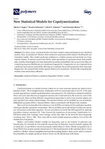
it can be concluded that (6) can be approximated by a Gaussian distribution [10] as also illustrated in Fig. 2. Note that for details on the derivation of (6) the reader is referred to [10]. The following remark is in order: Remark 1: No exact analytical results seem to exist for PLLs with low-pass filters1 . Nevertheless, the distribution in (6) seems to be a good approximation of experimentally obtained histograms of the phase error in such PLLs [12, pp. 112-117]. Remark 2: The block diagram in Fig. 3 does not correctly depict the use of a PLL in communication systems. As shown in Fig. 3 in practical communication systems the PLL is used to lock on to a reference signal generated by a very accurate crystal oscillator. The exact details of this PLL model is still a work in progress and more details will be provided in the next version of this report. 1
PLLs with first-order low-pass filters are most often used.
5
4
α =100 s
αs=30
3.5
α =10 s
α =3 s
3
α =1 s
α =0.5 s
α =0
2.5
p(∆θ)
s
2
1.5
1
0.5
0 −1
Fig. 2.
−0.8
−0.6
−0.4
−0.2
0
0.2
∆θ(t) normalized to π
0.4
0.6
0.8
1
Tikhonov distribution for different values of αs .
(t)
y(t)
Accurate low frequency crystal oscillator with frequency c
w(t)
C(t)
u(t)
L(t)/
!"
L(t)
L(t)
vco c
Fed back to the system but the details are yet unknow Fig. 3.
VCO
The practical implementation of phase-locked loop.
V. F REE RUNNING O SCILLATOR P HASE N OISE M ODEL The output of a noisy oscillator is given by [3] ζ(t) = (1 + ϵ(t)) cos(ωosc t + θ(t)),
(10)
6
where ϵ(t) and θ(t) are real random processes (RPs) that denote amplitude and phase fluctuations, respectively, and ωosc is the oscillator’s central frequency. Since ϵ(t) has a negligible effect on the output signal compared to the phase noise θ(t), the complex valued output of the oscillator can be written as [13], [14] ψ(t) = ej(ωosc t+θ(t)) .
(11)
Different types of noises affect the oscillator circuitry, which are then integrated to produce the phase fluctuations in the oscillator output [4], [15]. In continuous time, the phase fluctuation is expressed by ∫
t
Ω(t´) dt´
θ(t) =
(12)
0
where Ω(t) is the noise in the circuit. The circuit noise is a result of different parameters such as thermal noise, fluctuations in the input voltage of VCO, etc. [16]. In most scenarios Ω(t) is assumed to be a stationary zero-mean Gaussian random process and can be white or colored depending on the source of the noise. The phase noise variation caused by the phase noise process during the time interval τ is defined as
∫
t+τ
∆θ(τ ) = θ(t + τ ) − θ(t) =
Ω(t´) dt´,
(13)
t
where ∆θ(τ ) is the phase noise innovation, which according to the properties of Ω(t), is a zero-mean Gaussian random variable. Thus, the phase noise process θ(t) can be classified as a fractional Brownian motion. Note that, the variance of ∆θ(τ ) and its correlation properties are dependent on Ω(t). Next, we focus on the discrete-time properties of the phase noise process.
A. Discrete-time Model Considering a sampling time T , (12) can be rewritten as θ(nT ) =
N ∫ ∑ n=1
nT
(n−1)T
Ω(t´) dt´ =
N ∑ n=1
∆θ(nT ),
(14)
7
where ∆θ(nT ) denotes the sampled phase innovation ∆θ(τ ) and can be modeled as a zero-mean Gaussian random variable, since summation of zero-mean Gaussian random variables is also a zeromean Gaussian random variable. Therefore, the phase noise in each sample is given by
θn = θn−1 + ∆θ(nT ).
(15)
Using simple algebraic manipulations the autocorrelation of ∆θ(nT ), R∆θ (n, n+M ) can be calculated as 2 R∆ (n, n + M ) = π
∫
∞
SΩ (ω) 0
cos(M T ω)(1 − cos(T ω)) dω, ω2
(16)
where SΩ (ω) is the PSD of the circuit noise. The autocorrelation of ∆θ(nT ) for white circuit noise Ω(t) with constant PSD can be determined as
SΩ (ω) = k ⇒ R∆θ (M ) =
kT 0
if M = 0 .
(17)
if M ̸= 0
As it can be seen, the variance of ∆θ(nT ) is a linear function of the sampling time T . For this case, the phase noise process is a special case of discrete fractional Brownian motion known as random walk or the Wiener Process.
B. Future Work As it is discussed before, white noise is not the only type of noise that affects the oscillator circuitry. Empirical measurements of the phase noise show that flicker noise also plays an important part in the overall spectrum of phase noise. Thus, in order to have a more accurate model of phase noise, the effect of flicker noise must be also considered. Accordingly, the autocorrelation of phase noise innovation in this case needs to be derived. This is one of the many aspects of oscillator phase noise modeling that are being considered within the context of the MAGIC project.
8
VI. C ONCLUSION In this report we have summarized the phase noise models available in the literature. The constantphase and uniformly distributed phase noise models have been applied in the literature for performing information theoretical analyses due to their simplicity. However, as discussed these two models fail to accurately capture the properties of the phase noise process in communication systems. Next, the closed-loop and free-running oscillator phase noise models have been discussed, where it is highlighted that the Tikhonov distribution can accurately model the phase noise innovation in closedloop communication systems, e.g., when a PLL is applied to compensate the effect of phase noise. In the case of open-loop oscillators, the result of our investigation shows that the Wiener random walk model has been widely accepted as an accurate statistical representation of phase noise.
R EFERENCES [1] J. J. Kim, Y. Lee, and S. B. Park, “Low-noise CMOS LC oscillator with dual-ring structure,” IEEE Electronics Letters, vol. 40, no. 17, Aug. 2004. [2] J. H. G. Dauwels, “On graphical models for communications and machine learning: Algorithms, bounds, and analog implementation,” A dissertation submitted to the Swiss Federal Institute of Technology, Zurich for the degree of Doctor of Sciences ETH Zurich, pp. 161–166, May 2006. [3] M. Meyr and S. A. Fechtel, Synchronization in Digital Communications, Volume 1: Phase-, Frequency-Locked-Loops, and Amplitude Control.
New York, John Wiley & Sons, 1990.
[4] D. Leeson, “A simple model of feedback oscillator noise spectrum,” Proc. IEEE, vol. 54, no. 2, pp. 329 – 330, Feb. 1966. [5] A. Demir, A. Mehrotra, and J. Roychowdhury, “Phase noise in oscillators: a unifying theory and numerical methods for characterization,” IEEE Trans. Circuits Syst. I, Fundam. Theory Appl., vol. 47, no. 5, pp. 655 –674, May 2000. [6] A. Hajimiri and T. Lee, “A general theory of phase noise in electrical oscillators,” IEEE J. Solid-State Circuits, vol. 33, no. 2, pp. 179 –194, Feb. 1998. [7] L. Tomba, “On the effect of wiener phase noise in OFDM systems,” IEEE Trans. Commun., vol. 46, no. 5, pp. 580 –583, May 1998. [8] F. Munier, T. Eriksson, and A. Svensson, “An ICI reduction scheme for OFDM system with phase noise over fading channels,” IEEE Trans. Commun., vol. 56, no. 7, pp. 1119 –1126, 2008. [9] A. Lapidoth, “On phase noise channels at high SNR,” Information Theory Workshop, 2002, pp. 20–25, Oct. 2002.
9
[10] A. J. Viterbi, “Phase-locked loop dynamics in the presence of noise by fokker-planck techniques,” Proceedings of IEEE, pp. 1737–1753, 1963. [11] A. Mehrotra, “Noise analysis of phase-locked loops,” IEEE Trans. on Circ. and Systems I: Funda. Theory and Appl., vol. 49, no. 9, Sep. 2002. [12] A. Viterbi, Principles of Coherent Communication. McGraw-Hill, 1966. [13] G. Klimovitch, “A nonlinear theory of near-carrier phase noise in free-running oscillators,” in Proc. IEEE Intl. Conf. on Circuits Systs., Mar. 2000, pp. 1 –6. [14] S. Rytov, Principles of Statistical Radiophysics 2: Correlation Theory of Random Processes. New York: Springer, 1988, vol. 2. [15] A. Chorti and M. Brookes, “A spectral model for rf oscillators with power-law phase noise,” IEEE Trans. Circuits Syst. I, Reg. Papers, vol. 53, no. 9, pp. 1989 –1999, Sep. 2006. [16] F. Herzel, “An analytical model for the power spectral density of a voltage-controlled oscillator and its analogy to the laser linewidth theory,” IEEE Trans. Circuits Syst. I, Fundam. Theory Appl., vol. 45, no. 9, pp. 904 –908, Sep. 1998.