VAR models for the simulation of sea and wind state parameters ... In this work the use of vector autorregresive (VAR) and Regime Switching VAR models for the ...
Marine Technology and Engineering – Guedes Soares et al. (Eds) © 2011 Taylor & Francis Group, London, ISBN 978-0-415-69808-5
On the use of Vector Autoregressive (VAR) and Regime Switching VAR models for the simulation of sea and wind state parameters Sebastián Solari Universidad de Granada, Grupo de Dinámica de Flujos Ambientales, Granada, Spain Universidad de la República, IMFIA, Montevideo, Uruguay
Pieter H.A.J.M. van Gelder Delft University of Technology, Faculty of Civil Engineering and Geosciences, Delft, The Netherlands
ABSTRACT: The simulation of long (several years) time series of multivariate wave and wind state parameters has many applications in coastal and ocean engineering, including coastal morphology, transportation and energy exploitation studies, amongst others. In this work the use of vector autorregresive (VAR) and Regime Switching VAR models for the simulation of wave height, period and direction, and wind speed and direction, is studied. In order to normalize and stationarize the series, non-stationary mixture uni-variate distributions are fitted to the above five variables. Then three different VAR models (one standard model and two regime switching models) are fitted and new time series are simulated. Finally, an in depth analysis of the long term simulations is performed, in order to study its ability to reproduce the behavior of the original series. It is found that VAR models are able to capture main features of the original series, but they fail in reproducing some of the persistence regimes and some aspects of the bi-variate distributions. On the other hand, although Regime Switching VAR models improve some aspects of the simulations, they produce some unexpected behavior in the correlation of the simulated series.
1
INTRODUCTION
Simulation of time series of wave and wind parameters has many applications. Some of them are the design and management of harbors and waterways, the study of coastal morphology and the design of shore protection structures, the design, construction and operation of off-shore structures, etc. (Guedes Soares and Cunha 2000; Stefanakos and Belobassakis 2005). This work focuses on the study of a methodology for the simulation of new time series of the variables that defines the sea and wind states on deep waters, i.e.: spectral significant wave height H m 0 , peak period Tp , mean wave direction θ M , wind speed VW and wind direction θW . For the application and verification of the methodology a hindcasted time series is used. It corresponds to 13 years of 3 hours states, taken at the Gulf of Cádiz (36.5ºN, 6.5ºW), Spain. First, the five variables are normalized and stationarized. For this non-stationary parametric marginal distributions functions of the variables are used. Then, for modeling time dependence and interdependence of the normalized variables, the use of three Vector Autoregressive (VAR) models
is studied: a standard VAR model, and two Regime Switching VAR models, the Self Exiting Threshold VAR model (TVAR) and the Markov Switching VAR model (MSVAR). The objective is to study the ability of the different VAR models to reproduce the behavior of the original time series when they are used for long term simulations (several years). For this, simulated time series are compared with original ones in terms of its marginal distributions, its auto- and cross- correlation functions, and its persistence regimes over different thresholds. The rest of the document is organized as follows. Section 2 presents a brief revision of previous work on the use of autoregressive models for the simulation of multivariate met-ocean variables. In sections 3 to 5 the methodology used for the simulation is introduced as well as the structure of the different models used. Estimation of the parameters of the models for the study case is dealt with in sections 6 to 8. Once parameters are estimated new time series are simulated. The comparison of the new series with the original ones is done at section 9. Finally, a discussion of the results is done at section 10, while main conclusions of this work are summarized at section 11.
217
For the sake of readability of this document, many of the graphical results that partially justify the conclusions, as well as some details of the models used, are skipped. 2
BACKGROUND
This works focus on the multivariate simulation of time series of met-ocean variables by means of autoregressive models. The use of univariate autoregressive (AR) models for the simulation of significant wave height was presented in Guedes Soares and Ferreira (1996) and Guedes Soares et al. (1996). In Scotto and Guedes Soares (2000) the analysis is extended to the use of univariate self exiting threshold autoregressive (TAR) models. More recently Cai et al. (2007) analyze the use of AR models for the simulation of time series of environmental variables. With regards to multivariate simulation, Guedes Soares and Cunha (2000) use bivariate autoregressive models for the simulation of wave height and peak period time series. Stefanakos and Belobassakis (2005) use a vector autoregressive moving average model to the simulation of wave height, peak period and wind speed, while Cai et al. (2008) use a bivariate AR model for the study of wave heights and storm surges. Main differences of this work with previous ones are: (a) the analysis of TVAR and MSVAR models for 5-variate met-ocean variables, (b) the method used for normalization of the variables, and (c) the in depth analysis performed on the simulated series. In our work this analysis comprises several aspects not usually covered in previous works: probability distribution of the persistence regimes, marginal bivariate distributions of the normalized as well as of the original variables, and the ability of the model to reproduce the variability actually observed on the climatic variables (i.e. some years are more severe than others). This in depth analysis gives a better idea of the applicability and the limitation of the VAR models for met-ocean variables simulation than that obtained by only comparing autocorrelations and first moments of the original and simulated distributions. 3
METHODOLOGY
The proposed methodology comprises three steps: (a) Non-stationary distributions functions and normalization of the variables. For each one of the variables under study a non-stationary distribution function is fitted Vi (t ) ∼ Fi (Vi t ) . Using this function, variables are normalized by means of
(
)
Zi (t ) = Φ −1 Fi (Vi (t ) | t )
(1)
where Φ( ) is the standard normal univariate distribution. Non-stationary functions used in this work are introduced in section 4, the fitting of the functions to the data is presented on section 6, and the analysis of the normalized variables is shown in section 7. (b) Vector Autoregressive Models (VAR). These models are used to explain the time dependence and the inter-dependence of the normalized variables. First a order p VAR linear model is fitted (VAR( p ) ). Then, two different regime switching versions are fitted: a Self Exiting Threshold VAR model (TVAR( R ) ), and a Markov Switching VAR model (MSVAR( K R p ) ), where K R is the number of regimes of the models. The structure of the different models is introduced in section 5, while the estimation of its parameters is shown in section 8. (c) Simulation. The simulation of new time series comprises two steps. First, one of the VAR models is used for the simulation of a new time series of the normalized variables { i }. Then normalized variables are transformed to the original ones by means of the non-stationery distributions Vi Fi 1( (Zi ) | t ) . The simulated time series obtained with the different models are analyzed on section 9. 4
PROBABILITY DISTRIBUTIONS
Here the univariate marginal distribution functions used for normalization of the variables are described. Variables under study are H m 0 , Tp , θ M , VW and θW . Four different stationary and non-stationary distribution functions are used for the normalization of these five variables. These distributions are shown next. The parameters of these distributions are estimated through maximum likelihood. 4.1
c-GPD model
The distribution used for H m 0 and VW is the same that was used by (Solari and Losada 2011c). This distribution consists of a mixture of a truncated central distribution function for the central part, and two generalized Pareto distributions (GPD) for the tails. The distribution is ⎧ fm x )Fc (u1 ) x < u1 ⎪ f x) = ⎨ fc x ) u1 ≤ x ≤ u2 ⎪ f x ) ( − F ( u )) x > u2 c ⎩ M where fc is the density function selected for the central part, fm is the lower tail GPD and fM is
218
the upper tail GPD; u1 and u2 are lower and upper thresholds where the central distribution is truncated; Fc (u1 ) and 1 − Fc (u2 ) are scale constants for the lower and upper GPD respectively. For the density function (2) to be continuous and to have lower bound equal to zero, the following relations must be fulfilled (Solari and Losada 2011a; Solari and Losada 2011b)
σ1
ξ1u1 ξ1
F (u1 ) 1 − Fc (u2 ) σ2 = u1 fc (u1 ) fc u2 )
For modeling wave heights H m 0 a Log-Normal (LN) distribution is taken for the central function fc , and the resulting model is called LN-GPD. For wind speeds VW central distribution fc is taken to be a biparametric Weibull distribution (WB), and the resulting model is called WB-GPD. LN distribution has position parameter μLN and scale parameter σ LN > 0; the WB distribution has scale parameter αWB > 0 and shape parameter βWB > 0 ; the minimum GPD fm has shape parameter ξ1, scale parameter σ 1 ≥ 0 and position parameter u1; the maximum GPD fM has shape parameter ξ2 , scale parameter σ 2 ≥ 0 and position parameter u2 . In order to simplify the analysis the position parameters of both GPD, u1 and u2, are replaced by Z1 and Z2 , where ui Fc−1( (Zi )), being Φ the univariate standard normal distribution (see Solari and Losada 2011c). Then Z1 and Z2 are assumed to be constants, while the remaining parameters are time varying. Parameters of the LN-GPD distribution are ( μLN , σ LN , ξ2 , Z1, Z2 ), while those of the WB-GPD distribution are (α LN , β LN , ξ2 , Z1, Z2 ). Parameters μLN , σ LN , αWB , βWB and ξ2 are time varying, and are expressed as Fourier series
θ
Nk
θ a 0 + ∑ (θ
π
+θ
k =1
π
)
(3)
where t is on annual scale, and as a consequence only variations of periods less or equal to one year are taken into account (seasonal variations).
4.3
For both mean wave direction θ M and wind direction θW a mixture of four stationary normal distributions, truncated at 0 and 360 , is used 4
f x ) = ∑ α i fN i x x))⎡⎣ FN i ( i =1
5
−1
(5)
VECTOR AUTOREGRESSIVE MODELS
Autoregressive models give the value of the current observation as a linear function of past observations and a white noise. Vector Autoregressive models are an extension of autoregressive models for multivariate data. Here, three different models are considered. First, the classical Vector Autoregressive model of finite order p ( VAR( p ) ). Secondly two regime switching non-linear models constructed using the classical one: the Self Exciting Threshold Vector Autoregressive model of K R regimes and order p ( TVAR( R ) ), and the Markov Switching Vector Autoregressive model of K R regimes and order p (MSVAR( K R p ) ). These two model are based on the definition of different regimes. For each regime a VAR( p ) model isused, and as a consequence these two models are piecewise linear. For a description of vector autoregressive models the reader is referred to Lu¨tkepohl (2005). 5.1
VAR(p) model
The Vector Autoregressive model of order p is given by (see e.g.: Lu¨tkepohl (2005). p
yt
For the peak period Tp a mixture model composed by two LN distributions is defined. The model is ) fLN2 x )
) FN i ( ) ⎤⎦
where fN and FN are the probability density function (PDF) and the cumulative distribution function (CDF) of the normal distribution, and ∑ i4=1 α i = 1. The distribution has position parameters μNi and scale parameters σ Ni > 0 , with i = 1, 2, 3, 4 , and proportion parameters α i with 3 i = 1, 2, 3, being α 4 ∑ i 1 α i . Circular distributions for the direction variables will not be considered in this phase.
4.2 Bi log-normal model
f x ) = α fLN N1 x ) + (
Tetra truncated normal model
(4)
The parameters of the distribution are ( μ1 , σ 1, μ2 , σ 2 , α ), with σ 1,σ 2 > 0 and 0 α 1. All parameters are time varying and are expressed as Fourier series using (3).
∑ Ai yt i =1
i
+ ut
(6)
where yt ( y t , , yKt )′ is a vector of dimensions ( ), being K the number of variables; each Ai is a matrix of autoregressive coefficients, of dimensions ( ) ; ν (ν1, ,ν K )′ is a vector of dimension ( ) that allows for a non zero mean E ( yt ) ; and ut (u t , , uKt )′ is a K—dimensional white noise, also called innovation process or error, that
219
must fulfill E (ut ) = 0, E (u u ′ ) = Σ and E (u u ′ ) = 0 t t u t s for s ≠ t . In this work the parameters of the VAR( p ) model are estimated through Least Square (see Lu¨tkepohl 2005, Ch. 3). For this the model is expressed on matrix notation as Y = BZ U , where Y ( y1, , yT ), B ( , A1, , Ap ) , Zt [1 yt , , yt p +1 ]′ , Z (Z0 , Z1, , ZT −1 ) and U (u1, , uT ) , being T the number of observations available for estimation. Then, autoregresg sive parameters are estimated as Bˆ = YZ −11( ′ )−1; while the covariance matrix Σ u of the withe noise ˆ as ut is estimated through the errors Uˆ = Y − BZ ˆ ˆ ′ /( − + 1). Σˆ u = UU For defining the order p of the model that should be used it is possible to use the Bayesian Information Criteria BIC = −2 LLF + log(T )N p , where LLF is the log likelihood function and N p is the number of parameters of the model. Procedure is as follows: first model parameters are estimated for a series of orders p; then, LLF and BIC are estimated for each one of the models and the one with the lower BIC is selected as the “optimum” model. Assuming that the white noise follows a multivariate normal distribution of zero mean and covariance Σˆ u, the LLF is T
(f
LLF = ∑ l t =1
( | 0, Σˆ u ))
ˆ where fM MVN V ( ˆ | 0, Σ u ) is the density function of the multivariate normal distribution. 5.2
TVAR(KR,p) model
Threshold VAR models assume that there exists more than one possible regime for the system, and that at each time t the regime is defined by the value taken by the variable z at time t d , where d is the delay. When z is one of the variables of the regression, the model is called Self Exiting. This last case is the one studied here. The structure of the TVAR( R ) model is p
yt
( j)
∑ Ai( j ) yt i =1
i
+ ut( j )
if
rj
< zt − d ≤ rj (7)
where the set rj are the thresholds that defines the different regimes. Once that the number of regimes K R , the set of thresholds rj , the delay d , and the variable z used to identify the regimes are all defined, it is possible to estimate the autoregressive parameter and the covariance matrix of each regime in the same way it was done for the VAR model, using the Least Square method.
Here BIC is used for estimation of z , d , rj . To calculate the BIC of the TVAR model: (a) the LLF is estimated using a multivariate normal distribution for each regime, and (b) the number of parameters N p includes the parameters of all regimes. Then, given the number of regimes K R , for each one of the possible variables z a set of thresholds rj and a set of delays d are defined. Then, BIC is estimated for each possible model, and the one with the lower BIC is selected. This is repeatedwith different number of regimes, and again the one with the lower BIC is taken as the “optimum” model. This procedure is similar to that used by Tsay (1998), but in this case BIC is used for selecting the model, while Tsay used the mean square error. 5.3
MSVAR(KR,p) model
In the Markov Switching VAR model it is assumed the existence of an unobserved variable t that determines the regime at each time steps, and that this variables follows a discrete Markov process. Again, for each regime j a VAR model is defined. Then, the MSVAR( K R p ) is defined as p
yt
( j)
∑ Ai( j ) yt i =1
i
+ ut( j )
if
st
j
(8)
where the unobserved variable st follows a Markov process with transition matrix Ps , which has to be estimated on basis of the observed variables yt . There are two possible approaches for parameter estimation of MSVAR models: the use of maximum likelihood method, through a EM algorithm (see e.g. Hamilton 1990), or the use of Bayesian estimation procedure, through the use of Markov Chain Monte Carlo (MCMC) methods (see e.g. Albert and Chib 1993; Harris 1999). In this work the later approach is used. Again, the BIC is used for the selection of number of regimes K R and of the order p of the model. However in this case the likelihood function of the joint distribution of the observed and unobserved variables is used for the calculation of the BIC, and as a consequence the BIC obtained here can not be compared with those obtained for the VAR and TVAR models. The joint likelihood function is n
f Yn s
sn λ ) = f Yn Sn λ )P P((s ( s1 )∏ P(s P ( t st 1 ) t =2
(9) where
220
f Yn Sn λ
n
f (Y (Yr Sr λ ) ∏ f yt Yt t r +1
1
st λ ) (10)
with f Yr Sr λ ) being the likelihood of the first r observations and f yt Yt 1 st λ ) is the likelihood of the remaining observations conditional to the regimes and the previous observations, P( s1 ) is the marginal probability of the regimes and P ( st st 1 ) is the transition probability from st−1 to st . It should be noted that the estimation of the absolute likelihood of the observed variables would require the integration of (9) on all the possible realizations of st . 6
8 4
Hm0 [m]
2
0.4 0.2 0,1
DISTRIBUTIONS FITTING
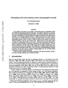
The parameters of the marginal distributions of the five variables are obtained through maximum likelihood. For the non-stationary distributions different models are fitted, varying the order of approximation of the Fourier series between 0 and 4 . For each model the BIC is estimated, and the one with the lower BIC is selected. The procedure is similar to that used in Solari and Losada (2011c). Models give a very good fitting for the five variables under study. Figures 1 and 2 show the model obtained for H m 0 . In figure 1 the annual mean probability density function (PDF) and cumulative distribution function (CDF) are presented. It is noticed that the model fits very well the data, except for the mode of the model, which is approximately 0.1 m smaller than the empirical mode. To verify that the model is able to capture the seasonal behavior of the variable, non-stationary empiri-
1 Hm0 Data Non stationary LN−GPD Model 0.5
0
0
1
2
3
4
5
Hm0 [m] Hm0 Data
0.99 0.9 0.5 0.1 0.01
Non Stationary LN−GPD Model
.1
.2
.4 .6 .8 1 Hm0 [m]
1 0.8 0.6
2
4
6 8 10
Figure 1. Annual probability density functions PDF (top) and cumulative distribution function CDF (bottom) for H m 0 .
0
0.2
0.4 0.6 Time [years]
0.8
1
Figure 2. Empirical (gray) and modeled (black) quantiles of 1, 5 , 10, 25 , 50 , 75 , 90 , 99 and 99.9% for H m 0 as a function of time.
cal and modeled quantiles are plotted in figure 2, where agreement between both is noticeable. A similar analysis (not shown here) is performed for the other four variables with similar results. 7
NORMALIZED DATA SERIES
By means of (1), and using the marginal distributions fitted in the previous section, the data series are normalized, obtaining the normalized variables ZH , ZT , Zθ M , ZV , and ZθW . First what can be noticed is that the normalization procedure is actually capable of producing standard normal distributions. Figure 3 shows the CDF of the normalized variables on normal probability paper. It is observed that they follow a standard normal distribution expect for probabilities lower than 0.1% or higher than 99.9%. Figure 4 shows the time series of the normalized variable ZH . It is noticed that, although there are no seasonal variations in the normalized time series (middle and bottom panels show the variable and the moving average of the mean and the standard deviation in annual scale), there are some important inter-annual variations that the transformation is not able to cope with. For example, the first two years of the series show higher values than the others (top panel). A complete analysis of the time series of the five normalized variables was also performed. Stationarity of the mean, the standard deviation and the auto- and cross-correlation were studied using the methodology described in van Gelder et al. (2007). In general terms no seasonal variations are observed in the mean and the standard deviation of the variables ZH , ZT are ZV , i.e. they can be assumed weakly stationary. However, some
221
seasonal variations are observed in the time series of Z0 M and ZθW . These variations are not considered significant and are overlooked. However, they could be avoided by using a non-stationary version of the tetra truncated normal model (5). With regards to correlations, it is noticed that autocorrelations of variables ZH and ZT show seasonality, while crosscorrelations ( H T ) , ( H V ) and ( T V ) show some non-stationary behavior but no clear seasonal pattern can be recognized.
It is concluded that the marginal non-stationary distributions can be used for the transformation of the original non-stationary variables into standard normal weakly stationary variables. However, there is non-stationarity remaining in the time dependence structure of the normalized variables that may justify the use of time varying models when modeling the time-dependence structure of the normalized variables. 8 8.1
Probability
0.999 0.99
VAR model
The parameters of the VAR( p ) model are estimated through the least square method described on section 5, for order p between 1 and 8. For each model the BIC is calculated, and the lower BIC is obtained with p = 7.
0.90 0.50 0.10 0.01 0.001 −4
AUTOREGRESSIVE MODELS PARAMETERS ESTIMATION
8.2 −2
0 Z
2
4
ZH
Figure 3. CDF of the normalized variables in normal probability paper.
TVAR model
First a two regimes model (KR = 2) is fitted using several different variables z for defining the regimes: wave height H m 0 , normalized wave height ZH , peak period Tp , normalized period ZT , wind speed VW , normalized wind speed ZV , wave
4 2 0 −2 −4 0
0.5
1
1.5
2
2.5
3
ZH
Time
3.5 x 10⁴
4 2 0 −2 −4 0
0.2
0.4 0.6 Time [year]
0.8
1
0.2
0.4 0.6 Time [year]
0.8
1
1 0.5 0 0
Figure 4. Time series of the normalized variable ZH (top), normalized variable on annual scale (middle), and 90 days moving average of the mean and the standard deviation (bottom).
222
responds to wave heights and wind speeds higher than the mean, and peak period lowerthan the mean, all characteristics of sea conditions. Regime two can be seen as an intermediate regime, with average wave heights and periods, and moderate to high wind speeds. 8.4
Residuals analysis
A usual way to evaluate the quality of the autoregressive models is to study the residuals. In this work residuals where supposed to follow a normal distribution in order to estimate the LLF of the autoregressive models. Figure 5 shows the residuals of of ZH obtained with the VAR(7 ) model. It is notice that residuals do not show significant autocorrelation (middle panel), and that 80% of them follows a normal distribution (lower panel). The lower and upper 10% of the residuals also tend to follow a normal distributions, but with higher variance. This is considered to be a consequence of the non-stationarity observed on the variance of the residual (upper panel). Also an analysis on the stationarity and independence of all the remaining residuals was performed. It was observed that residuals show some non-stationarity. This is coherent with the
2 UH
steepness H m Tp2 and pseudo normalized wave steepness ZH ZT . According to the BIC the best fit model is obtained when z is wind speed VW , although good fits are also obtained when taking z as the normalized wind speed or the wave height. In all the three cases optimum delay d is 1 and optimum order p is 7 . After that a three regime (K R = 3 ) model is fitted, but in this case only significant wave height H m 0 , wind speed VW and normalized wind speed ZV are evaluated as regime defining variables z . Again best fit, evaluated through BIC, is obtained when z VW with delay d = 1 and order p = 7. BIC of the three regimes model TVAR( ) is smaller than the BIC of the two regimes model TVAR( ) , which in turn is smaller than the BIC of the standard model VAR(7 ) . Therefore model TVAR( ) is selected, with z VW and ( 1 2) = ( ). Results obtained indicate that the time dependence structure of the variables depends on the intensity of the wind. Three different structures are identified: one for soft winds, with VW 3.8 m/s (Beaufort under 4), other for relatively strong winds VW 7.1 m/s (Beaufort over 5), and a last one for intermediate winds speeds 3.8 /s < VW < 7.1 .1 m/s (Beaufort between 4 and 5). It was noticed that for every studied TVAR model the optimum order p was 7 and the optimum delay d was 1, except when the pseudo-steepness was used for z , for which optimum delay d was 3 .
0 −2
8.3
MSVAR model
0 Sample Autocorrelation
MSVAR models with two and three regimes are studied. In both cases order p varying between 1 and 8 is evaluated and BIC is estimated using (9). The model with the minimum BIC is MSVAR(3, 7 ). In the MSVAR model the vector ν ( j ) gives an idea of the physical meaning of each regime. Table 1 presents the three ν ( j ) vectors obtained for the MSVAR(3, 7 ). It is seen that regime one corresponds to wave heights lower than the mean, with peak periods over the mean and wind speeds lower than the mean, all of them characteristics of swell conditions. Regime three on the other hand cor-
ZH
ZT
ZθM
ZV
ZθW
1 2 3
–0.105 0.023 0.308
0.102 0.038 –0.842
0.215 –0.091 –0.694
–0.282 0.188 0.228
–0.078 0.053 0.006
0.4 0.6 Time [year]
0.8
1
1
0.5
0 0
6
12
18
24 30 36 Lag [hours]
42
48
54
60
Probability
0.999
Table 1. ν vector for the three regimes of the model MSVAR(3,7). Reg.
0.2
0.90 0.50 0.10 0.001 −2
−1
0 UH
1
2
3
ˆ H obtained with VAR(7 ) model Figure 5. Error U ˆ H (middle), CDF of U ˆ H in (top), autocorrelation of U normal probability paper (bottom).
223
non-stationarity observed in the dependence structure of the normalized variables. However, from the point of view of this work, i.e. the long term simulation of new series for engineering applications, it is considered that the best way of evaluating adequacy of the models is by studying the new simulated time series. This is conducted in the next section.
1
PDF
0.8 0.6 0.4 0.2 0
9
SIMULATION
Three time series of the normalized variables, of 500 years each, are simulated using the three autoregressive models fitted in previous section. Then, these series are transformed to the original variables by means of the marginal distributions. Next, the simulated series are compared with the original ones in terms of its marginal distributions (uni- and bi-variate) and its interannual variability, of its persistence regimes and of its auto- and cross-correlations. 9.1
Univariate marginal distributions and interannual variability
Ferreira and Guedes Soares (2002) pointed out that probability models for sea state parameters should be able to reproduce the interannual variability that is characteristic of environmental variables. This variability is evident when one compares the PDF of different measured years. Here, it is verified that the simulated series share the same mean annual PDF as the original series, and that they also reproduce most of the interannual variability registered on the original time series. In figure 6 the annual PDF of each of the 500 years simulated with the VAR(7 ) model are presented, along with the PDF of the 13 measured years and its mean annual PDF. Results obtained for the other variables, as well that those obtained with models TVAR( ) and MSVAR(3, 7 ), have the same behavior as those presented here. First, it is noticed that the simulated series are able to reproduce the mean annual PDF of the measured series. On the other hand, the simulations show a significant variation in the annual PDF. The annual PDF of the simulated series produce a cloud around the annual mean PDF of the measured data that includes most of the measured annual PDF. However, there are at least two years of measured data whose PDF can not be reproduce by the simulated series. Those two years correspond to the first two years of the measured series, for which severer weather was observed, i.e. higher wave heights and wind speed and lower peak period.
0
1
2 Hm0 [m]
3
4
0.25
PDF
0.2 0.15 0.1 0.05 0
5
10 Tp [s]
15
20
Figure 6. Interanual variability of the anual PDF for H m 0 (top) and Tp (bottom). Grey: annual PDF for each simulated year; Broken Black: anual PDF for each measured year; Continuous Black: mean anual measured PDF.
9.2 Bivariate distributions It is important that the simulated series reproduce not only the marginal bivariate distributions of the measured data but also its marginal multivariate distributions, since the latter contain information about the joint occurrence of values of the variables. Among the multivariate distributions, bivariate distributions are the the easiest to evaluate graphically and are the most familiar for the coastal engineer, therefore here the ability of the simulated series to reproduce the original bivariate distributions is analyzed. The 10 possible bivariate distributions were analyzed. Here only the two most commonly used bivariate distributions are included. Figures 7 and 8 show bivariate distributions of ( H m 0 ,Tp ) and ( H m 0 ,VW ) respectively, for both the original and the normalized variables. It was observed that data series simulated with VAR(7 ) model reproduce well those bivariate distributions of the normalized variables whose behavior is similar to that of a multivariate normal distribution, i.e. with only one mode and with constant dependence structure for the whole range of values of the variables. When the bivariate dis-
224
2.5
2
2
1
−1
0.5
−2 5
10 Tp [s]
−3 −3
15
3
2.5
2
2
1
−2
−1
0 Z(Tp)
1
2
3
−2
−1
0 Z(Tp)
1
2
3
−2
−1
0 Z(Tp)
1
2
3
−2
−1
0 Z(Tp)
1
2
3
m0
)
3
Z(H
1.5
0
1
−1
0.5
−2 5
10 Tp [s]
−3 −3
15
3
2.5
2
2
1 m0
)
3
Z(H
1.5
0
1
−1
0.5
−2
0
5
10 Tp [s]
−3 −3
15
3
2.5
2
2
1 )
3
m0
Hm0 [m]
0
1
0
Hm0 [m]
Z(H
1.5
0
Hm0 [m]
m0
)
3
1.5
Z(H
Hm0 [m]
3
0
1
−1
0.5
−2
0
5
10 Tp [s]
−3 −3
15
Figure 7. Bivariate distribution of Hm0 − Tp (left) and of ZH − ZT (right), obtained with the measured data (top) and with the data simulated with the VAR (second from top), the TVAR (third from top) and the MSVAR (bottom) models.
225
3
2.5
2
2
1 Z(Hm0)
Hm0 [m]
3
1.5
0
1
−1
0.5
−2
0
0
5
−3 −3
10
−2
−1
0 Z(VW)
1
2
3
−2
−1
0 Z(VW)
1
2
3
−2
−1
0 Z(VW)
1
2
3
−2
−1
0 Z(VW)
1
2
3
3
3
2.5
2
2
1 Z(Hm0)
Hm0 [m]
VW [m/s]
1.5 1
−1
0.5
−2
0
0
5
−3 −3
10 VW [m/s]
3
3
2.5
2
2
1 Z(Hm0)
Hm0 [m]
0
1.5
0
1
−1
0.5
−2
0
0
5
−3 −3
10
3
3
2.5
2
2
1 Z(Hm0)
Hm0 [m]
VW [m/s]
1.5
0
1
−1
0.5
−2
0
0
5
VW [m/s]
−3 −3
10
Figure 8. Bivariate distribution of Hm0 − VW (left) and of ZH − ZV (right), obtained with the measured data (top) and with the data simulated with the VAR (second from top), the TVAR (third from top) and the MSVAR (bottom) models.
226
tribution shows multimodality or its dependence structure depends on the value of the variables, as is the case of (ZH ,ZT ) and (ZH ,ZV ) respectively, the model is unable to capture this behavior. Model TVAR( ) has a better performance capturing the varying dependence structure of the (ZH ,ZV ) distribution, but it is unable to reproduce the bimodality of the (ZH ,ZT ) distribution. MSVAR(3, 7 ) on the other hand is capable of reproducing the bimodality of the (ZH ,ZT ) distribution and also improves the results obtained with the TVAR( ) in the (ZH ,ZV ) distribution. However, the improvement obtained with the regime switching models in the representation of the bivariate distribution of the normalized variables, does not translate into a significant improvement in the representation of the bivariate distributions of the original variables. It is observed that the bivariate distributions obtained with the three autoregressive models are very similar. All of them reproduce the main features of the bivariate distribution of the measured data, but still all of them fail in reproducing some details of the distributions, as can be the increase on the dependence between H m 0 and Tp for storm conditions (high wave height and low periods). 9.3 Persistence regimes Persistence regimes over different thresholds are useful for the estimation of the operationality of navigation channels, for the planning of marine operations, or for the estimation of the availability of renewable energy resources as wind and waves. Therefore, it is important that the simulation is as accurate as possible on the representation of the persistence regimes of the variables. Persistence regimes of the three simulated series are very similar. In general terms it is observed that persistence regimes are well reproduced by the simulated series for thresholds close to the mean of the variables. As the threshold increases the difference between the persistence regimes of the measured
and the simulated series increases too. The general trend is to produce shorter persistences than those observed in the measured data. As an example of this, figure 9 shows persistence regimes of H m 0 and VW over thresholds corresponding to nonexceedance probabilities 0.5 and 0.9. Although it has not been verified, it is suspected that the observed trend to produce shorter persistences than observed may be partially caused by the inability of the model in reproducing all the observed interannual variability of the variables, i.e. if more severe years could be simulated it is expected that also longer persistence over high thresholds would occur. 9.4
Auto- and cross-correlation
Figure 10 shows auto- and cross-correlation functions, for lag up to hours, obtained with the measured and the simulated series. It is observed that VAR(7 ) model is the one that better reproduce the correlation structure of the measured series. In the case of the normalized variables the correlations obtained with the simulated series are almost identical to those obtainedwith the measured series. However, in case of the original variables, some significant difference are observed for those correlations that involves any of the direction variables. This may be because in this work direction variables are treated as linear variables, when in fact they are circular variables. Maybe the correlation structure of the simulated series could be improved by using circular model for direction variables. On the other hand, regime switching models ( ) and MSVAR(3, 7 ) produce unexpected effects on the correlation structure of the simulated series. In particular it is noted that the series simulated with the MSVAR(3, 7 ) model have higher cross-correlation between H m 0 and the variables Tp , θ M and θW , than that observed on the measured series. Additionally, it shows positive cross-correlation between Tp and VW , while the
0.08
0.08
0.08
0.06
0.06
0.06
0.04
0.04
0.04
0.02
0.02
0.02
0
0
0.1
0
0.08 0.06 0.04
0
24 48 72 Persistence of Hm0 over 0.9 m [hours]
Figure 9.
96
0.02 0
24 48 72 Persistence of Hm0
96
0
24 48 72 Persistence of VW over 5.4 m/s [hours]
over 2 m [hours]
96
0
0
24 48 72 Persistence of VW over 10 m/s [hours]
Persistence of Hm0 and VW over thresholds corresponding to mean annual probability 0.5 and 0.9.
227
96
0.5 0
W M
W
0.5 0
12 24 36 time lag [hrs]
1 0.5 0 1 0.5 0 1 0.5 0 1 0.5 0
0.5 0
12 24 36 time lag [hrs]
48
CCF (Hm0;θW) CCF (Hm0;θM)
0.2 0.1 0
W
0.3
0
p
0 0.1
−0.1 −0.2 0
0.1
0
−0.3 −0.6
0.6 0.3
0.3
0.1
24
36
48
0
0
−0.1 −48 −36 −24 −12 0 12 time lag [hrs]
24
36
48
24
36
48
−0.3
0.8
0.3
0.4 0 0.3
0
0 0
−0.3
0
−0.1
1
CCF (T ;V )
0
0 −48 −36 −24 −12 0 12 time lag [hrs]
48
W
ACF θ )
m0
ACF Z(H
0.4
−0.1
CCF (θ ;θ )
1
ACF Z(Tp)
−0.2
p
ACF V
W
W
CCF (T ;θ )
1
0
CCF (θM;VW)
0
0.1
0
−0.1
CCF (VW;θW)
p
0.5
0.1
CCF Z(VW;θW) CCF Z(θ ;V ) CCF Z(T ;V ) CCF Z(H ;θ ) CCF Z(Hm0;θM) M W p W m0 W
ACF θ
M
1
ACF Z(θM)
;T )
m0
0.5 0
ACF Z(VW)
0.8
CCF Z(Tp;θM) CCF Z(H ;V ) CCF Z(H ;T ) m0 W m0 p
ACF T
p
1
ACF Z(θW)
CCF (H
0
0
0.2
CCF (Tp;θM) CCF (Hm0;VW)
0.5
0
0.4
CCF Z(θM;θW) CCF Z(T ;θ ) p
m0
ACF H
1
0
−0.3
0.4
0.1
0.2 0 −48 −36 −24 −12
0
12
time lag [hrs]
24
36
48
0
−0.1 −48 −36 −24 −12
0
12
time lag [hrs]
Figure 10. Auto- and cross correlation functions of the original (top) and normalized (bottom) variables. Lags expressed in hours. Blue circles: measured data; continuos line: VAR model simulated series; dashed line: TVAR model simulated series; dotted line: MSVAR model simulated series.
measured data shows negative cross-correlation (with higher winds sea condition is observed, while with lower winds swell prevails). 10
DISCUSSION
The proposed univariate marginal distribution functions provide a good fit to the measured data
series, and gives a valid alternative to the methods used by other authors (Cunha and Guedes Soares 1999; Stefanakos and Belobassakis 2005) for the normalization and stationarization of the data series. However, the proposed method has two limitations. First, it does not account for interannual variations and trends on the series. Secondly, it is unable to produce fully non-stationary series.
228
First mentioned limitation can easily be overcome by allowing the parameters of the distributions to have different time variation structure. Without background modifications of the proposed models, just by including additional factors on equation (3), the parameters can be allowed to vary with periods greater than one year (e.g.: multi year cyclic variations), to have nonperiodic dependence on time (e.g.: to have trends), and even to be a function of covariables (e.g.: climatic indexes). On the other hand, the second mentioned limitation does not have a straightforward solution. The detailed study done about the stationarity of the normalized time series shows that these can only be considered weakly non-stationary, and that they have time varying dependence structure. This last aspect can not be taken into account with the proposed normalization procedure. In order to cope with it, it would be necessary to use time varying models for modeling the dependence structure (e.g. time varying VAR models). It was found that, when using the VAR model for modeling the time dependence structure of the series, most of its behavior can be explained. New simulated series obtained with the fitted VAR model reproduce satisfactorily the auto- and crosscorrelation structure of the original series, as well as its univariate marginal distributions, and to some extend its interannual variability and its persistence regimes. Studied regime switching models (TVAR and MSAR) were found more able in reproducing the behavior of the bivariate marginal distributions of the normalized variables. Particulary the MSVAR is able to capture both bimodal and dependence varying bivariate distributions. This however does not translate into a significant improvement of agreement between the measured and the simulated bivariate distributions of the original variables. 11
CONCLUSIONS
In summary, a methodology based on the use of non-stationary distributions and autoregressive models was introduced, which can be used for the simulation of long-term series of 5-variate metocean variables. Through an in depth analysis of the simulated series main limitations of the simulation procedure, when used for engineering applications, were identified. Amongst them is the inability of the models to reproduce the observed persistence regimes for high thresholds of the variables. It has been shown that the use of regime switching models do not necessarily produce better simulated series, although fitting errors are reduced, and better agreement is achieved between the measured
and simulated bivariate distributions of the normalized variables. Given the unexpected behavior of the correlations observed in the series simulated with the regime switching models, its use in our case study is discouraged. At least two possible work lines were identified and discussed in previous sections that could improve the simulation of met-ocean variables: (a) to introduce long term variations, trends and covariables into the parameters of the marginal univariate distributions, and (b) to use time varying VAR models for modeling time dependence structure of the normalized series.
ACKNOWLEDGEMENTS Sebastián Solari would like to acknowledge to Ministerio de Educación (Spanish Ministry of Education), for the financial support provided through the FPU scholarship (reference number AP200903235), and to the Consejería de Economía, Innovación y Ciencia of Junta de Andalucía (Ministry of Economy, Innovation and Science of the Andalusian Government, Spain) for financial supporting his stay at Delft University of Technology. Wave and wind data series used in this work were kindly provided by Puertos del Estado (Spanish Port Authority).
REFERENCES Albert, J.H. and S. Chib (1993). Bayes inference via gibbs sampling of autoregressive time series subject to markov mean and variance shifts. Journal of Business and Economic Statistics 11(1), 1–15. Cai, Y., B. Gouldby, P. Dunning, and P. Hawkes (2007). A simulation method for flood risk variables. In 2nd Institute of Mathematics and its Applications International Conference on Flood Risk Assessment, 4th September 2007 , University of Plymouth, England. Cai, Y., B. Gouldby, P. Hawkes, and P. Dunning (2008). Statistical simulation of flood variables: incorporating short-term sequencing. Journal of Flood Risk Management 1, 3–12. Cunha, C. and C. Guedes Soares (1999). On the choice of data transformation for modelling time series of significant wave height. Ocean Engineering 26, 489–506. Ferreira, J. and C. Guedes Soares (2002). Modelling bivariate distributions of significant wave height and mean wave period. Applied Ocean Research 24, 31–45. Guedes Soares, C. and A.M. Ferreira (1996). Representation of non-stationary time series of significant wave height with autoregessive models. Probabilistic Engineering Mechanics 11, 139–148. Guedes Soares, C., A.M. Ferreira, and C. Cunha (1996). Linear models of the time series of significant wave height on the southwest coast of portugal. Coastal Engineering 29, 149–167.
229
Guedes Soares, C. and C. Cunha (2000). Bivariate autoregressive models for the time series of sognificant wave height and mean period. Coastal Engineering 40, 297–311. Hamilton, J.D. (1990). Analysis of time series subject to change in regime. Journal of Econometrics 45, 39–70. Harris, G.R. (1999). Markov chain monte carlo estimation of regime switching vector autoregressions. Astin Bulletin 29(1), 47–79. Lu¨tkepohl, H. (2005). New Introduction to Multiple Time Series Analysis. Springer-Verlag. Scotto, M. and C. Guedes Soares (2000). Modelling the long-term series of significant wave height with non-linear threshold models. Coastal Engineering 40, 313–327. Solari, S. and M.A. Losada (2011a). Identification of minimum, mean and maximum wave regimes. part i: Model description. To be submitted to Coastal Engineering. Solari, S. and M.A. Losada (2011b). Identification of minimum, mean and maximum wave regimes. part ii: Application. To be submitted to Coastal Engineering.
Solari, S. and M.A. Losada (2011c). Non-stationary wave height climatie modeling and simulation. To be submitted to Coastal Engineering. Stefanakos, C.N. and K.A. Belobassakis (2005, June 12-16). Nonstationary stochastic modelling of multivariate long-term wind and wave data. In Proceeding of 24th International Conference on Offshore Mechanics and Arctic Engineering (OMAE2005). Halkidiki, Greece. Tsay, R.S. (1998). Testing and modeling multivariate threshold models. Journal of the American Statistical Association 93, 1188–1202. van Gelder, P., W. Wang, and J. Vrijling (2007). Extreme Hydrological Events: New Concepts for Security, Volume 78 of Earth and Environmental Sciences, Chapter Statistical estimation methods for extreme hydrological events, pp. 199–252. Springer.
230