Radio Networks. Monireh ... AbstractâIn a cognitive radio network, a secondary user learns ...... when we talk about an attacker employing PROLA, we assume.
1
Optimal Online Learning with Randomized Feedback Graphs with Application in PUE Attacks in CRN
arXiv:1709.10128v1 [cs.NI] 28 Sep 2017
Monireh Dabaghchian, Amir Alipour-Fanid, Kai Zeng, Qingsi Wang, Peter Auer
Abstract—In a cognitive radio network, a secondary user learns the spectrum environment and dynamically accesses the channel where the primary user is inactive. At the same time, a primary user emulation (PUE) attacker can send falsified primary user signals and prevent the secondary user from utilizing the available channel. The best attacking strategies that an attacker can apply have not been well studied. In this paper, for the first time, we study optimal PUE attack strategies by formulating an online learning problem where the attacker needs to dynamically decide the attacking channel in each time slot based on its attacking experience. The challenge in our problem is that since the PUE attack happens in the spectrum sensing phase, the attacker cannot observe the reward on the attacked channel. To address this challenge, we utilize the attacker’s observation capability. We propose online learning-based attacking strategies based on the attacker’s observation capabilities. Through our analysis, we show that with no observation within the attacking slot, the attacker loses on the regret order, and with the observation of at least one channel, there is a significant improvement on the attacking performance. Observation of multiple channels does not give additional benefit to the attacker (only a constant scaling) though it gives insight on the number of observations required to achieve the minimum constant factor. Our proposed algorithms are optimal in the sense that their regret upper bounds match their corresponding regret lower-bounds. We show consistency between simulation and analytical results under various system parameters.
I. I NTRODUCTION Nowadays the demand to wireless bandwidth is growing rapidly due to the increasing growth in various mobile and IoT applications, which raises the spectrum shortage problem. To address this problem, Federal Communications Commission (FCC) has authorized opening spectrum bands (e.g., 35503700 MHz and TV white space) owned by licensed primary users (PU) to unlicensed secondary users (SU) when the primary users are inactive [1, 2]. Cognitive radio (CR) is a key technology that enables secondary users to learn the spectrum environment and dynamically access the best available channel. Meanwhile, an attacker can send signals emulating the primary users to manipulate the spectrum environment, preventing a secondary user from utilizing the available channel. This attack is called primary user emulation (PUE) attack [3, 4, 5, 6, 7, 8, 9]. Existing works on PUE attacks mainly focus on PUE attack detection [10, 11, 12] and defending strategies [5, 6, 7, 8]. However, there is a lack of study on the optimal PUE attacking strategies. Better understanding of the optimal attacking strategies will enable us to quantify the severeness or impact
of a PUE attacker on the secondary user’s throughput. It will also shed light on the design of defending strategies. In practice, an attacker may not have any prior knowledge of the primary user activity characteristics or the secondary user’s dynamic spectrum access strategies. Therefore, it needs to learn the environment and attack at the same time. In this paper, for the first time, we study the optimal PUE attacking strategies without any assumption on the prior knowledge of the primary user activity or secondary user accessing strategies. We formulate this problem as an online learning problem. We also need to mention that the words play, action taking, and attack are used interchangeably throughout the paper. Similar idea holds between actions and channels. Different from all the existing works on online learning based PUE attack defending strategies [5, 6, 7, 8], in our problem, an attacker cannot observe the reward on the attacked channel. Considering a time-slotted system, the PUE attack usually happens in the channel sensing period, in which a secondary user attempting to access a channel conducts spectrum sensing to decide the presence of a primary user. If a secondary user senses the attacked channel, it will believe the primary user is active so that it will not transmit the data in order to avoid interfering with the primary user. In this case, the PUE attack is effective since it disrupts the secondary user’s communication and affects its knowledge of the spectrum availability. In the other case, if there is no secondary user attempting to access the attacking channel, the attacker makes no impact on the secondary user, so the attack is ineffective. However, the attacker cannot differentiate between the two cases when it launches a PUE attack on a channel because no secondary user will be observed on the attacked channel no matter a secondary user ever attempted to access to the channel or not. The key for the attacker to launch effective PUE attacks is to learn which channel or channels a secondary user is most likely to access. To do so, the attacker needs to make observations on the channels. As a result, the attacker’s performance is dependent on its observation capability. We define the observation capability of the attacker as the number of the channels it can observe after it launches the attack within the same time slot. We propose two attacking schemes based on the attacker’s observation capability. In the first scheme called Attack-OR-Observe (AORO), an attacker if attacks, cannot make any observation in a given time slot due to the short slot duration in highly dynamic systems [13] or when the channel switching time is long. We call this attacker an attacker with
no observation capability (since no observation is possible if it attacks). To learn the most rewarding channel though, the attacker needs to dedicate some time slots for observation only without launching any attacks. On the other hand, an attacker could be able to attack a channel in the sensing phase and observe other channels in the data transmission phase within the same time slot if it can switch channels fast enough. We call this attacking scheme, Attack-But-Observe-Another (ABOA). For the AORO case, we propose an online learning algorithm called POLA -Play or Observe Learning Algorithm- to dynamically decide between attack and observation and then to choose a channel for the decided action, in a given time slot. Through theoretical analysis, √ we prove that POLA achieves a ˜ 3 T 2 ) where T is the number of slots regret in the order of O( the CR network operates. Its higher slope regret is due to the fact that it cannot attack (gain reward) and observe (learn) simultaneously in a given time slot. We show the optimality of our algorithm by matching its regret upper bound with its lower bound. For the ABOA case, we propose PROLA -Play and Random Observe Learning Algorithm- as another online learning algorithm to be applied by the PUE attacker. PROLA dynamically chooses the attacking and observing channels in each time slot. The PROLA learning algorithm’s observation policy fits a specific group of graphs called time-varying partially observable feedback graphs [14]. It is derived in [14] √ that ˜ 3 T 2 ). these feedback graphs lead to a regret in the order of O( However, our algorithm, PROLA, is based on a new theoretical √ ˜ T ). framework and we prove its regret is in the order of O( √ ˜ T) We then prove its regret lower bound in the order of Ω( which matches its upper bound and shows our algorithms’ optimality. Both algorithms proposed address the attacker’s observation capabilities and can be applied as optimal PUE attacking strategies without any prior knowledge of the primary user activity and secondary user access strategies. We further generalize PROLA to multi-channel observations where an attacker can observe multiple channels within the same time slot. By analyzing its regret, we come to the conclusion that increasing the observation capability from one to multiple channels does not give additional benefit to the attacker in terms of regret order. It only improves the constant factor of the regret. Our main contributions are summarized as follows: •
•
We formulate the PUE attack as an online learning problem without any assumption on the prior knowledge of either primary user activity characteristics or secondary user dynamic channel access strategies. We propose two attacking schemes, AORO and ABOA, that model the behavior of a PUE attacker. For the AORO, a PUE attacker, in a given time slot, dynamically decides either to attack or observe; then chooses a channel for the decision it made. While in the ABOA case, the PUE attacker dynamically chooses one channel to attack but chooses at least one other channel to observe within the same time slot.
We propose an online learning algorithm POLA for the AORO case. POLA achieves an optimal learning regret in √ ˜ 3 T 2 ). We show its optimality by matching the order of θ( its regret lower and upper bounds. • For ABOA case, we propose an online learning algorithm, PROLA, to dynamically decide the attacking and observing channels. We prove √ that PROLA achieves an ˜ T ) by deriving its regret optimal regret order of θ( upper bound and lower bound. This shows that with an observation capability of at least one, there is a significant improvement on the performance of the attacker. • The algorithm and the analysis of the PROLA are further generalized to multichannel observation case. • Theoretical contribution: For PROLA, despite observing the√actions partially, it achieves an optimal regret order √ of ˜ 3 T 2 ). ˜ T ) which is better than a known bound of θ( θ( We accomplish it by proposing randomized time-variable feedback graphs. • We conduct simulations to evaluate the performance of the proposed algorithms under various system parameters. Through theoretical analysis and simulations under various system parameters, we have the following findings: • With no observation at all in the attacking slot, the attacker loses on the regret order. While with the observation of at least one channel, there is a significant improvement on the attacking performance. • Observation of multiple channels in the PROLA algorithm, does not give additional benefit to the attacker p in terms of regret order. The regret is proportional to 1/m, where m is the number of channels observed by the attacker. This non-linear relationship implies, the regret reduces more when the number of observing channels increases in the beginning. As more observing channels are added, the reduction in the regret becomes marginal. Therefore, a relatively small number of observing channels is sufficient to approach a small constant factor. √ • The attacker’s regret is proportional to K ln K, where K is the total number of channels. The rest of the paper is organized as follows. Section II discusses the related work. System model and problem formulation are described in Section III. Section IV proposes the online learning-based access strategies applied by the attacker and derives the regret bounds. Simulation results are presented in section V. Finally, section VI concludes the paper and discusses future work. •
II. R ELATED W ORK A. PUE Attacks in Cognitive Radio Networks Existing work on PUE attacks mainly focus on PUE attack detection [10, 11, 12] and defending strategies [5, 6, 7, 8]. There are few works discussing attacking strategies under dynamic spectrum access scenarios. In [5, 6], the attacker applies partially observable Markov decision process (POMDP) framework to find the attacking channel in each time slot. It is assumed that the attacker can observe the reward on the attacking channel. That is, the attacker knows if a secondary user is ever trying to access a channel or not. In [7, 8], it is
assumed that the attacker is always aware of the best channel to attack. However, there is no methodology proposed or proved on how the best attacking channel can be decided. The optimal PUE attack strategy without any prior knowledge of the primary user activity and secondary user access strategies is not well understood. In this paper, we fill this gap by formulating this problem as an online learning problem. Our problem is also unique in that the attacker cannot observe the reward on the attacking channel due to the nature of PUE attack.
23, 24]. In jamming attacks, an attacker can usually observe the reward on the attacking channel where an ongoing communication between legitimate users can be detected. Also it is possible for the defenders whether they are defending against a jammer or a PUE attacker to observe the reward on the accessed channel. PUE attacks are different in that the attacker attacks the channel sensing phase and prevents a secondary user from utilizing an available channel. As a result, a PUE attacker cannot observe the instantaneous reward on the attacked channel. That is, it cannot decide if an attack is effective or not.
B. Multi-armed Bandit Problems There is a rich literature about online learning algorithms. The most related ones to our work are multi-armed bandit (MAB) problems [15, 16, 17, 18, 19]. The MAB problems have many applications in cognitive radio networks with learning capabilities [7, 20, 21]. In such problems, an agent plays a machine repeatedly and obtains a reward when it takes a certain action at each time. Any time when choosing an action the agent faces a dilemma of whether to take the best rewarding action known so far or to try other actions to find even better ones. Trying to learn and optimize his actions, the agent needs to trade off between exploration and exploitation. On one hand the agent needs to explore all the actions often enough to learn which is the most rewarding one and on the other hand he needs to exploit the believed best rewarding action to minimize his overall regret. For most existing MAB frameworks as explained, the agent needs to observe the reward on the taken action. Therefore, these frameworks cannot be directly applied to our problem where a PUE attacker cannot observe the reward on the attacking channel. Most recently, Alon et al. generalize the cases of MAB problems into feedback graphs [14]. In this framework, they study the online learning with side observations. They show in their work that if an agent takes an action without observing its reward, but observes the reward of all the other √ actions, it can achieve an optimal regret in the ˜ T ). However, the agent can only achieve a regret order √ of O( ˜ 3 T 2 ) if it cannot observe the rewards on all the other of O( actions simultaneously. In other words, even one√missing edge ˜ 3 T 2 ). in the feedback graph leads to the regret of O( In this paper, we propose two novel online learning policies. The first one, POLA, for the case when either only observation or attack is possible within a √ time slot, is shown to achieve ˜ 3 T 2 ). We then advance this a regret in the order of O( theoretical study by proposing a strategy, PROLA, which is suitable for an attacker with higher observation capabilities. We prove √ that PROLA achieves an optimal regret in the order ˜ T ) without observing the rewards on all the channels of O( other than the attacking one simultaneously. In PROLA, the attacker uniform randomly selects at least one channel other than the attacking one to observe in each time slot. Our framework is called randomized time-variable feedback graph. C. Jamming Attacks There are several works formulating jamming attacks and anti-jamming strategies as online learning problems [21, 22,
D. Adaptive Opponents Wang et al. study the outcome/performance of two adaptive opponents when each of the agents applies a no regret learning-based access strategy [21] . One agent tries to catch the other on a channel and the other one tries to evade it. Both learning algorithms applied by the opponents not only are no regret algorithms but also are designed for oblivious environments. In other words, each of the learning algorithms are designed for benign environments and non of them assumes an adaptive/learning-based opponent. It is shown in this work, that both opponents applying a no-regret learning-based algorithm, reach an equilibrium which is in fact Nash Equilibrium in that case. In other words, despite the fact that the learning-based algorithms applied are originally proposed for oblivious environments, the two agents applying these algorithms act reasonably well achieving an equilibrium. Motivated by this work, in our simulations in Section V, we have considered a learning-based secondary user. More specifically, even though we proposed learning-based algorithms for oblivious environments, but in the simulations, we evaluate its performance in an adaptive environment. The simulation results show the rationality of the attacker that even against an adaptive opponent (learning-based cognitive radio) performs well and achieves a regret below the derived upper bound. III. S YSTEM M ODEL AND P ROBLEM F ORMULATION We consider a cognitive radio network consisting of several primary users, multiple secondary users, and one attacker. There are K (K > 1) channels in the network. We assume the system is operated in a time-slotted fashion. A. Primary User In each time slot, each primary user is either active (on) or inactive (off). We assume the on-off sequence of PUs on the channels is unknown to the attacker a priori. In other words, the PU activity can follow any distribution or can even be arbitrary. B. Secondary User The secondary users may apply any dynamic spectrum access policy [25, 26, 27]. In each time slot, each SU conducts spectrum sensing, data transmission, and learning in three consecutive phases as shown in Fig. 1(a).
Table I: Main Notation
Figure 1: Time slot structure of a) an SU and b,c,d) a PUE attacker. At the beginning of each time slot, each secondary user senses a channel it attempts to access. If it finds the channel idle (i.e., the primary user is inactive), then accesses this channel; Otherwise, it remains silent till the end of the current slot in order to avoid interference to the primary user. At the end of the slot, it applies a learning algorithm to decide which channel it will attempt to access in the next time slot based on its past channel access experiences. We assume the secondary users cannot differentiate the attacking signal from the genuine primary user signal. That is, in a time slot, when the attacker launches a PUE attack on the channel a secondary user attempts to access, the secondary user will not transmit any data on that channel. C. Attacker We assume a smart PUE attacker with learning capability. We do not consider attack on the PUs. The attacker may have different observation capabilities. Observation capability is defined as the number of channels the attacker can observe after the attack period within the same time-slot. Observation capabilities of the attacker are impacted by the overall number of it’s antennas, time slot duration, switching time, etc. Within a time-slot, an attacker with at least one observation capability conducts three different operations. First in the attacking phase, the attacker launches the PUE attack by sending signals emulating the primary user’s signals [6] to attack the SUs. Note that, in this phase, the attacker has no idea if its attack is effective or not. That is, it does not know if a secondary user is ever trying to access the attacking channel or not. In the observation phase, the attacker is supposed to observe the communication on at least one other channel. The attacker may detect a primary user signal, a secondary user signal, or nothing on the observing channel. The attacker applies its observation in the learning phase to optimize its future attacks. At the end of the learning period, it decides which channels it attempts to attack and observe in the next slot. Fig. 1(b) shows the time slot structure for an attacker with at least one observation capability. If the attacker has no observation capability, at the end of each time slot it still applies a learning strategy based on which, it decides whether to dedicate next time slot for attack or observation and chooses a channel for either of them. Fig. 1(c,d) show the time slot structure for an attacker with no observation capability. As shown in these two figures, the attacker conducts only either attack or observation at each time slot.
T K k It Jt R γ η pt (i) qt (i) ωt (i) δt
total number of time slots total number of channels index of the channel index of the channel to be attacked index of the channel to be observed total regret of the attacker in Algorithm 1 exploration rate used in algorithm 2 learning rate used in Algorithms 1 and 2 attack distribution on channels at time t in Algorithms 1 and 2 observation distribution on channels at time t in Algorithm 1 weight assigned to channel i at time t in Algorithms 1 and 2 Observation probability at time t in Algorithm 1
D. Problem Formulation Since the attacker needs to learn and attack at the same time and it has no prior knowledge of the primary user activity or secondary user access strategies, we formulate this problem as an online learning problem. We consider T as the total number of time slots the network operates. We define xt (j) as the attacker’s reward on channel j at time slot t (1 ≤ j ≤ K, 1 ≤ t ≤ T ). Without loss of generality, we normalize xt (j) ∈ [0, 1]. More specifically: ( 1, SU is on channel j at time t xt (j) = (1) 0, o.w. Suppose the attacker applies a learning policy ϕ to select the attacking and observing channels. The aggregated expected reward of attacks by time slot T is equal to: " T # X Gϕ (T ) = Eϕ xt (It ) (2) t=1
The attacker’s goal is to maximize the expected value of the aggregated attacking reward, thus to minimize the throughput of the secondary user. maximize
Gϕ (T )
(3)
For a learning algorithm, regret is commonly used to measure its performance. The regret of the attacker can be defined as follows. Regret = Gmax − Gϕ (T )
(4)
where Gmax = max j
T X
xt (j)
(5)
t=1
The regret measures the gap between the accumulated reward achieved applying a learning algorithm and the maximum accumulated reward the attacker can obtain when it keeps attacking the single best channel. This regret is usually called the weak regret [17]. Then the problem can be transformed to minimize the regret. minimize Gmax − Gϕ (T ) Table I summarizes the main notation used in this paper.
(6)
observation capability, provides insight to find the approximate number of observations required to achieve the minimum constant factor in the regret upper bound. A. Attacking Strategy 1: POLA Learning Algorithm
Figure 2: Decision Making process based on the POLA strategy: First the agent decides between play and observe, then for either of them chooses a channel dynamically.
POLA is an online learning algorithm for the learning of an agent with no observation capability. In other words, the agent cannot play and observe simultaneously. If modeled properly as a feedback graph as is shown in Appendix A, this problem can be solved based on the EXP3.G algorithm presented in [14]. However, our proposed learning algorithm, POLA, leads to a smaller regret constant compared to the one in [14] and it is much easier to understand. Based on the POLA attacking strategy, the attacker at each time slot decides between attacking and observation, dynamically. If it decides to attack, it applies an exponential weighting distribution based on the previous observations it has made. It chooses a channel uniformly at random if it decides to make an observation. Fig. (2) represents the decision making structure of POLA. The proposed algorithm is presented in Algorithm 1.
IV. O NLINE L EARNING -BASED ATTACKING S TRATEGY In this section we propose two novel online learning algorithms for the attacker. These algorithms do not require the attacker to observe the reward on the attacked channel. Moreover, our algorithms can be applied in any other application with the same requirements. The first algorithm proposed, POLA, is suitable for an attacker with no observation capability. For this attacker, either attack or observation is feasible within each time slot. Based on this learning strategy, the attacker decides at each time slot whether to attack or observe and chooses a channel for either of them, dynamically. The assumption here is that, any time the attacker decides to make observation, it observes only one channel since time slot duration has been considered short or switching costs are high compared to the time slot duration. The second algorithm, PROLA, is proposed for an attacker with at least one observation capability. Based on this learning policy, the attacker at each time, chooses channels dynamically for both attack and observation. In the following, we assume the attacker’s observation capability is one. We generalize it to multiple channel observation capability in Section IV-C. Both algorithms are considered as no-regret online learning algorithms in the sense that the incremental regret between two consecutive time slots diminishes to zero as time goes to infinity. The first√one, POLA, achieves an optimal regret ˜ 3 T 2 ). This higher slope arises from the in the order of O( fact that at each time slot, the attacker gains only some reward by attacking a channel without updating its learning or it learns by making observation without being able to gain any reward. PROLA,√is also optimal with the regret proved ˜ T ). Comparing these algorithms and in the order of O( the generalization of the latter together shows that, changing from no observation capability to one observation capability, there is a significant improvement in the regret order; This is in comparison to changing from one observation capability to multiple observation capability which does not give any benefits in terms of regret order. However, multiple channel
Algorithm 1: POLA, Play or Observe Learning Algorithm Parameter: η ∈ (0, 1/K] Initialization: ω1 (i) = 1, For each t = 1,� 2, ..., qT 1. Set δt = min 1, 3
i = 1, ..., K � K ln K . t
With probability δt decide to observe and go to step 2. With probability 1 − δt decide to attack and go to step 3. 2. Set 1 qt (i) = , i = 1, ..., K K Choose Jt ∼ qt and observe the reward xt (Jt ). For j = 1, 2, ..., K ( xt (j) , j = Jt x ˆt (j) = δt (1/K) 0, o.w. ωt+1 (j) = ωt (j) exp(ηˆ xt (j)) Go back to step 1. 3. Set ωt (i) pt (i) = K , P ωt (j)
i = 1, ..., K
j=1
Attack channel It ∼ pt and accumulate the unobservable reward xt (It ). For j = 1, 2, ..., K x ˆt (j) = 0 ωt+1 (j) = ωt (j) Go back to step 1.
Since the attacker is not able to attack and observe within the same time slot simultaneously, it needs to trade off between attacking and observation cycles. From one side the attacker needs to make observations to learn the most rewarding channel to attack. From the other side, it needs to attack often enough to minimize his regret. So, δt which represents the trade off between attack and observation needs to be chosen carefully. In step 2 of Algorithm 1, x ˆt (j) represents an unbiased estimate of the reward xt (j). In order to derive this value, we divide the xt (j) by the probability that this channel index is chosen to be observed which is equal to δt /K. This is because in order for each channel to be chosen to be observed, first the algorithm needs to decide to observe with probability δt and then to choose that channel for observation uniformly at random. For any agent that acts based on the Algorithm 1, the following theorem holds. Theorem 1. For any K ≥ 2 and for any η ≤ bound on the expected regret of Algorithm 1
1 K,
the upper
q +1)4 consider 3 3 (T K ln K >> K ln K which is equivalent to T >> K√ln K − 1 then the regret bound in the corollary is achieved. 4 27 � Proof of Theorem 1. The regret at time t is a random variable equal to, ( r(t) =
xt (j ∗ ) − EP OLA,A [xt (It )] ∗
, Attack ∗
xt (j ) − EP OLA,O [xt (It )] = xt (j ) , Observe
where j ∗ is the index of the best channel. The expected value of regret at time t is equal to: E [r(t)] = (1 − δt ) (xt (j ∗ ) − EP OLA,A [xt (It )]) + δt xt (j ∗ ) (9) where the expectation is w.r.t. to the randomness in the attacker’s attack policy. Expected value of accumulated regret, R, is, " T # X E [R] = E r(t) t=1
s 4 3 3 (T + 1) K ln K Gmax − E [GP OLA ] ≤ (e − 2)ηK + 4 K ln K 4 +
3√ ln K 3 + KT 2 ln K η 2
(7)
=
T X
(1 − δt ) (xt (j ∗ ) − EP OLA,A [xt (It )]) +
≤
xt (j ∗ ) −
t=1
T X
EP OLA,A [xt (It )] +
t=1
Corollary 1. For any T > 0 and the input parameter v u ln K u � q � η=u t 3 +1)4 K ln K (e − 2)K 34 (T + K ln K 4 Then p 3√ 3 Gmax − E[GP OLA ] ≤ ( 3(e − 2) + ) KT 2 ln K 2 holds for any arbitrary assignment of rewards. Proof of Corollary 1. We sketch the proof as follows. Since η ≤ 1/K, in order for the regret bound to be non-trivial, we � �(3/4) 6−e K ln K − 1 = 1.37K ln K − 1. Then need T ≥ 3(e−2) by getting the derivative, we find the optimal values for η. If we plug in the η the regret will be equal to, √ Gmax − E[GP OLA ] ≤ e − 2 K ln K sr 4 3 (T + 1) 3 + K ln K K ln K 3√ 3 + KT 2 ln K (8) 2 Also T is an upper bound on the Gmax since all the rewards are in [0, 1] and the attacker attacks for T time steps. If we √
T X
δt
t=1
(10)
holds for any assignment of rewards for any T > 0. By choosing appropriate values for η, the above upper bound on the regret can be minimized.
δt xt (j ∗ )
t=1
t=1 T X
T X
The inequality results from the fact that δt ≥ 0 and xt (j ∗ ) = 1. It is also assumed that xt (i) ≤ 1 for all i. Now the regret consists of two terms. The first one is due to not attacking the most rewarding channel but attacking some other low rewarding channels. The second term arises because of the observations in which the attacker gains no reward. We derive an upper bound for each term separately, then add them together. δt plays the key role in minimizing the regret. First of all, δt needs to be decaying since otherwise it leads to a linear growth of regret. So the key idea in designing a no-regret algorithm is to choose an appropriate decaying function for δt . From one side, slowly decaying δt is desired from learning point of view; however, it results in a larger value of regret since staying more in the observation phase precludes the attacker from launching attacks and gaining rewards. On the other hand, if δt decays too fast, the attacker settles in a wrong channel since it does not have enough time to learn the � q � K most rewarding channel. We choose δt = min 1, 3 K ln t and our analysis shows the optimality of this function in minimizing the regret. Below is the derivation of the upper bound for the first term of regret in equation (10). For a single t, K
X ωt (i) Wt+1 = exp(ηˆ xt (i)) Wt Wt i=1 =
K X i=1
pt (i) exp(ηˆ xt (i))
≤
K X
pt (i)[1 + ηˆ xt (i) + (e − 2)η 2 x ˆ2t (i)]
i=1
� X � K K X 2 2 ≤ exp η pt (i)ˆ xt (i) + (e − 2)η pt (i)ˆ xt (i) i=1
The upper bound on the second term of equation (10) is as follows. r T T 3 K ln K 3√ X X 3 ≤ KT 2 ln K δt = min 1, 2 t t=1
i=1
t=1
(11)
(16)
where PK the equalities follow from the definition of Wt+1 = i=1 ωt (i), ωt+1 (i), and pt (i), respectively in Algorithm 1. Also the last inequality follows from the fact that ex ≥ 1 + x. Finally, the first inequality holds since ex ≤ 1 + x + (e − 2)x2 for x ≤ 1. In this case, we need ηˆ xt (i) ≤ 1. Based on our algorithm, ηˆ xt (i) = 0 if i 6= Jt and for i = Jt we have ≤ ηK ηˆ xt (i) = η xδt (i) 1 δt , since xt (i) ≤ 1. This means that we
Summing up the equation (15) and equation (16) gives us the regret upper bound. �
tK
δt K.
1 K
should have η ≤ Since δt ≤ 1 we conclude that η ≤ By taking the ln and summing over t = 1 to T on both sides of equation (11), the left hand side (LHS) of the equation will be equal to the following, T X t=1
ln
WT +1 Wt+1 = ln Wt W1
x ˆt (j) − ln K
(12)
t=1
By combining (12) with (11), we have:
η
T X
x ˆt (j) − ln K ≤ η
t=1
T X K X
pt (i)ˆ xt (i)
t=1 i=1
+ (e − 2)η 2
T X K X
√ 3 Gmax − E [GA ] ≥ v KT 2 for some small constant v and it holds for some assignment of rewards for any T > 0.
pt (i)ˆ x2t (i)
�
Based on Theorem’s 1 and 2, the algorithm’s regret upper bound matches its regret lower bound which indicates POLA is an optimal online learning algorithm.
≥ ln ωT +1 (j) − ln K T X
Theorem 2. For K ≥ 2 and for any player strategy A, the expected weak regret of algorithm A is lower bounded by
Proof of Theorem 2. See Appendix.
= ln WT +1 − ln K
=η
Next is a theorem on the regret lower bound for this problem under which attacking and observation are not possible simultaneously.
(13)
t=1 i=1
We take the expectation w.r.t. the randomness in x ˆ, substitute j by j ∗ since j can be any of the actions, use the definition of EP OLA,A [xt (It )] and with a little simplification and rearranging the equation we get the following:
B. Attacking Strategy 2: PROLA Learning Algorithm In this section, we propose another novel online learning algorithm that can be applied by the PUE attacker with one observation capability. The proposed optimal online learning algorithm, called PROLA, at each time, chooses two actions dynamically to play and observe, respectively. The action to play is chosen based on an exponential weighting, while the other action for observation is chosen uniformly at random excluding the played action. The proposed algorithm is presented in Algorithm 2. Fig. 3 shows the observation policy governing the actions for K = 4 in a feedback graph format. In this figure, Yij (t) ∈ {0, 1} such that at each time for the chosen action i to be played, K X
Yij (t) = 1, i = 1, . . . , K t = 1, . . . , T (17) T j=1,j6=i X 1 ln K xt (j ∗ ) − EP OLA,A [xt (It )] ≤ (e − 2)ηK + For example, if channel 2 is attacked (i = 2), only one of the δ η t=1 t=1 t=1 t three outgoing edges from 2 will be one. This edge selection (14) which corresponds to the channel to be observed is chosen q uniformly at random equal to 1/K. We call this feedback T P 1 3 3 (T +1)4 K ln K The upper bound on is equal to + graph, a time-variable random feedback graph. Our feedback δt 4 K ln K 4 t=1 graph fits into the time-variable feedback graphs introduced in which gives us the following, [14] and based on the results derived in that work, the regret √ 3 2 ). However, based on ˜ T T upper bound of our algorithm is O( T X X ln K ∗ xt (j ) − EP OLA,A [xt (It )] ≤ + (e − 2)ηK our analysis, the √ upper bound on the attacker’s regret is in η ˜ T ) which shows a significant improvement. t=1 t=1 the order of O( s In other words, despite the fact that the agent makes only 4 3 (T + 1) 3 K ln K partial observation on the channels, it achieves a significantly + 4 K ln K 4 improved regret order. This has been possible due to the new (15) property we considered in the partially observable graphs. This
T X
T X
Similarly, we can minimize the regret bound by choosing an appropriate value for η. Corollary 2. For any T > 0, we consider T as an upper bound on the Gmax and consider the following value for η q ln K η = 2(e−2)(K−1)g Then p p Gmax − E[GP ROLA ] ≤ 2 2(e − 2) T (K − 1) ln K holds for any arbitrary assignment of rewards.
Figure 3: Channel observation strategy, K = 4
Proof of Corollary 2. We sketch the proof as follows. Since γ γ ≤ 1/2 and η ≤ 2(K−1) , in order for the regret bound to property is adding randomness which in the long run make full observation possible to the agent. Algorithm 2 : PROLA, Play and Random Observe Learning Algorithm Parameters: γ ∈ �(0, 1/2], i γ η ∈ 0, 2(K−1) Initialization: ω1 (i) = 1, For each t = 1, 2, ..., T
j=1
t
Proof of Theorem 3. By using the same definition for Wt = K P ωt (1) + · · · + ωt (K) = ωt (i) as in Algorithm 1, at each
γ K,
K
X pt (i) − γ/K Wt+1 exp(ηˆ xt (i)) = Wt 1−γ i=1 i = 1, ..., K ≤
2. Attack channel It ∼ pt and accumulate the unobservable reward xt (It ).
x ˆt (j) =
xt (j) (1/(K−1))(1−pt (j)) ,
j = Jt
0,
o.w.
ωt+1 (j) = ωt (j) exp(ηˆ xt (j)).
In Step 4 of Algorithm 2, in order to create x ˆt (j), an unbiased estimate of the actual reward xt (j), we divide the observed reward, xt (Jt ), by (1/(K − 1))(1 − pt (Jt ))which is the probability of choosing channel Jt to be observed. In other words, channel Jt will be chosen to be observed if it has not been chosen for attacking (1 − pt (Jt )) and second if it gets chosen uniformly at random from the rest of the channels, (1/(K − 1)).
K X pt (i) − γ/K
1−γ
i=1
[1 + ηˆ xt (i) + (e − 2)(ηˆ xt (i))2 ] � K η X ≤ exp pt (i)ˆ xt (i) 1 − γ i=1 � K (e − 2)η 2 X 2 + pt (i)ˆ xt (i) 1 − γ i=1
3. Choose a channel Jt other than the attacked one uniformly at random and observe its reward xt (Jt ) based on equation (1) 4. For j = 1, ..., K (
i=1
time t we have,
i = 1, ..., K
1. Set pt (i) = (1 − γ) PKωt (i) + ω (j)
ln K be non-trivial, we need g ≥ 16(K−1) . Then by getting e−2 the derivative, we find the optimal values for η. Also T is an upper bound on the g since all the rewards are in [0, 1] and the network runs for T time slots, which gives us the result. �
The equality follows from the definition of Wt+1 , ωt+1 (i), and pt (i) respectively in Algorithm 2. Also the last inequality follows from the fact that ex ≥ 1 + x. Finally, the first inequality holds since ex ≤ 1 + x + (e − 2)x2 γ for x ≤ 1. When η ≤ 2(K−1) , the result, ηˆ xt (i) ≤ 1 , follows from the observation that either ηˆ xt (i) = 0 or t (i) ηˆ xt (i) = η 1 x(1−p ≤ η(K − 1) γ2 ≤ 1, since xt (i) ≤ 1 (i)) t
K−1
γ and pt (i) = (1 − γ) PKωt (i) +K ≤ 1 − γ + γ2 ≤ 1 − γ2 . j=1 ωt (j) By taking the logarithm of both sides of (18) and summing over t from 1 to T , we derive the following inequality on the LHS of the equation, T X t=1
ln
Wt+1 WT +1 = ln Wt W1 ≥ ln ωT +1 (j) − ln K
γ , for the Theorem 3. For any K ≥ 2 and for any η ≤ 2(K−1) given randomized observation structure for the attacker the upper bound on the expected regret of Algorithm 2,
Gmax − E[GP ROLA ] ≤ 2(e − 2)(K − 1)ηGmax + holds for any assignment of rewards for any T > 0.
ln K η
(18)
=η
T X
x ˆt (j) − ln K.
t=1
As a result the inequality (18) will be equal to: T X t=1
x ˆt (j)−
T X K X t=1 i=1
pt (i)ˆ xt (i) ≤ γ
T X t=1
x ˆt (j)+
(19)
(e − 2)η
T X K X
pt (i)ˆ x2t (i) +
t=1 i=1
ln K η
pt (i)ˆ xt (i). We make
i=1
the pivotal observation that (20) also holds for x ´t (i) since η´ xt (i) ≤ 1, which is the only key to obtain (20). We also note that pt (i)´ x2t (i) =
i=1
= ≤
K X
i=1 K X
pt (i)ˆ x2t (i) − ft2 pt (i)ˆ x2t (i) −
i=1
=
pt (i)(ˆ xt (i) − ft )2
i=1
K X
K X
K X
p2t (i)ˆ x2t (i)
i=1
pt (i)(1 − pt (i))ˆ x2t (i)
(21)
i=1
Substituting x ´t (i) in equation (20) and combining with (21), we have K T T X X X pt (i)(ˆ xt (i) − ft ) (ˆ xt (j) − ft ) − t=1
=
T X
x ˆt (j) t=1 T X
≤γ
−
pt (i)ˆ xt (i)
x ˆt (j) −
t=1 K T X X
!
pt (i)(1 − pt (i))ˆ x2t (i) +
ln K η
(22)
Observe that x ˆt (j) is similarly designed as an unbiased estimate of xt (j). Then for the expectation with respect to the sequence of channels attacked by the horizon T , we have the following relations: # "K X pt (i)ˆ xt (i) = E[xt (It )] E[ˆ xt (j)] = xt (j), E i=1
and E
# pt (i)(1 −
pt (i))ˆ x2t (i)
=E
K X
# pt (i)(K − 1)x2t (i) ≤ (K − 1).
i=1
We now take the expectation with respect to the sequence of channels attacked by the horizon T in both sides of the last inequality of (22). On the left hand side, we have " T # " T K # X XX E x ˆt (j) −E pt (i)ˆ xt (i) t=1
The important observation is that, based on [14] such an algorithm, Algorithm �√ � 2, is expected to achieve a regret in the ˜ 3 T 2 since it can be categorized as a partially order of O observable graph. However, our analysis gives a tighter bound and shows not only it is tighter but also it achieves the regret order of fully observable graphs. This significant improvement has been accomplished by introducing randomization into feedback graphs. The following theorem provides the regret lower bound for this problem. Theorem 4. For any K ≥ 2 and for any player strategy A, the expected weak regret of algorithm A is lower bounded by √ Gmax − E[GA ] ≥ c KT
�
t=1 i=1
= Gmax − E[GP ROLA ]. And for the right hand side we have E[R.H.S] ≤ γ(Gmax − E[GP ROLA ])+
We generalize Algorithm PROLA to the case of an agent with multiple observation capability. This is suitable for an attacker with multiple observation capability when the attacker after the attack phase can observe multiple other channels within the same time-slot. At least one and at most K − 1 observations are possible by the agent (attacker). In this case, for 1 ≤ m ≤ K − 1 we have, K X
Yij (t) = m,
i = 1, . . . , K
t = 1, . . . , T.
(24)
j=1,j6=i
The probability of a uniform choice of observations at each K P time, Yij (t) = m is equal to K1 . Corollary 3 shows (m) j=1,j6=i the result of the analysis for m observations. Corollary 3. If the agent can observe m actions at each time, then the regret upper bound is the q following: p Gmax − E [GA ] ≤ 4 (e − 2) T K−1 m ln K
i=1
"
since Gmax can be substituted by T , the above relation gives us the proof assuming γ ≤ 1/2. �
C. Extension to Multiple Action Observation Capability
pt (i)ˆ xt (i)
t=1 i=1
"K X
ln K , η
Proof of Theorem 4. See Appendix.
i=1
+ (e − 2)η
(1 − γ)(Gmax − E[GP ROLA ]) ≤ (e − 2)(K − 1)ηT +
for some small constant c and it holds for some assignment of rewards for any T > 0.
t=1 i=1 T X K X t=1 i=1 K X
ln K η
Combining the last two equations we get, K P
Let x ´t (i) = x ˆt (i) − ft where ft =
K X
(e − 2)(K − 1)ηT +
(20)
(23)
This regret upper bound shows a faster convergence rate when making more observations. Proof of Corollary 3. We substitute 1/ (K − 1) by m/ (K − 1) in Step 4 of Algorithm PROLA since at each time, m actions are being chosen uniformly at random. Then the regret upper bound can be derived by similar analysis. � As our analysis shows, making multiple observations does not improve the regret in terms of its order in T compared to
the case of making only one observation. This means that only one observation and not more than that is required to make a significant improvement in terms of regret order reduction. The advantage of making more observations however is in reducing the constant coefficient in the regret. Making more observations leads to a smaller constant factor in the regret upper bound. This relationship is non-linear though. i.e., the q 1 which means that regret upper bound is proportional to m in order to make a large reduction in the regret in terms of its constant coefficient impact, only a few observations would suffice without requiring so many observation. Our simulation results in Section V-C provide more details on this non-linear relationship. V. P ERFORMANCE E VALUATION In this section, we present the simulation results to evaluate the validity of the proposed online learning algorithms applied by the PUE attacker. All the simulations are conducted in MATLAB and the results achieved are averaged over 10,000 independent random runs. We evaluate the performance of the proposed learning algorithms, POLA and PROLA, and √ compare them √ with their ˜ T ), respec˜ 3 T 2 ) and O( theoretical regret upper bounds O( tively. POLA and PROLA correspond to an attacker with no observation and one observation capability, respectively. We then examine the impact of different system parameters on the attacker’s performance. The parameters include the number of time slots, total number of channels in the network, and the distribution on the PU activities. We also examine the performance of an attacker with multiple observation capabilities. Finally we evaluate a secondary user’s accumulated traffic with and without the presence of a PUE attacker. K primary users are considered, each acting on one channel. The primary users’ on-off activity follows a Markov chain or i.i.d. distribution in the network. Also the PU activities on different channels are independent from each other. K idle probabilities are generated using MATLAB’s rand function, each denoting one PU activity on each channel if PUs follow an i.i.d. Bernoulli distributions. pI = [0.85 0.85 0.38 0.51 0.21 0.13 0.87 0.7 0.32 0.95] is a vector of K elements each of which denotes the corresponding PU activity on the K channels. If the channels follow Markov chains, for each channel, we generate three probabilities, p01, p10, and p1 as the transition probabilities from state 0 (on) to 1 (off), from 1 to 0, and the initial idle probability, respectively. The three vectors below, are examples considered to represent PU activities. p01 = [0.76 0.06 0.3 0.24 0.1 0.1 0.01 0.95 0.94 0.55], p10 = [0.14 0.43 0.23 0.69 0.22 0.59 0.21 0.58 0.34 0.73], and p1 = [0.53 0.18 0.88 0.66 0.23 0.87 0.48 0.44 0.45 0.88]. The PUE attacker employs either of the proposed attacking strategies, POLA, or PROLA. Throughout the simulations, when we talk about an attacker employing PROLA, we assume the attacker’s observation capability is one, unless otherwise stated. Since the goal here is to evaluate the PUE attacker’s performance, for simplicity we consider one SU in the network.
Throughout the simulations, we assume the SU employs an online learning algorithm called Hedge [16]. The assumption on the Hedge algorithm is that the secondary user is able to observe the rewards (PU activities) on all the channels in each time slot. Hedge provides the minimum regret in terms of both order and the constant factor among all optimal learning-based algorithms. As a result the performance of our proposed learning algorithms can be evaluated in the worst case scenario for the attacker. As explained in Section II, even though in our analysis we considered an oblivious environment, in the simulations we can consider an SU that runs Hedge (an adaptive opponent). This experimental setup adds value since it shows that our proposed online learningbased algorithms perform reasonably even against adaptive opponents by keeping the occurred regret below the theoretical bounds derived. A. Performance of POLA and the impact of the number of channels In this section, we evaluate the performance of the proposed algorithm, POLA and compare it with the theoretical analysis. Then examine the impact of the number of channels in the network on it’s performance. We consider K variable from 10 to 50. Fig. 4 (a) shows the overall performance of the attacker for both cases of i.i.d. and Markovian chain distribution of PU activities on the channels for K = 10. The attacker’s regret when PUs follow i.i.d. distribution and Markovian chain for different number of actions are shown in Fig. 4 (b) and (c), respectively. Since POLA has a regret with higher slope, in order to better observe the results, we have plotted the figures for T from 1 to 20, 000. We can observe the following from the figures. • Regardless of the PUs activity type, the occurred regret is below the regret upper bound achieved from the theoretical analysis. This can be seen by plugging in the values of K, m, and T in the regret upper bounds derived in Theorems 1 and 3.. • The regret on all three figures has a higher slope which also complies with our analysis. • As the number of channels increases the regret increases as well, as is expected based on the theoretical analysis from Corollary 1. • As the number of channels increases, the regret does not increase linearly with it. Instead, the increment in the regret becomes marginal which complies with the theoretical analysis. √ Based on Corollary 1 the regret is proportional to ( 3 K ln K). B. Performance of PROLA and the impact of the number of channels We compare the performance of the proposed learning algorithm, PROLA, with the theoretical analysis from section IV. We consider a network of K = 10 channels. Fig. 4(d) shows the simulation results. From the simulations we observe that the actual regret occurred in the simulations, is below the one achieved from the theoretical upper bound regardless of
(a) POLA Learning
(b) POLA, channel impact, i.i.d. PU
(c) POLA, channel impact, M.C. PU
(d) PROLA Learning
(e) PROLA, channel impact, i.i.d. PU
(f) PROLA, channel impact, M.C. PU
(g) PROLA, observation impact, i.i.d. PU
(h) PROLA, observation impact, M.C. PU
(i) Accumulated Traffic of an SU
Figure 4: Simulation results under different PU activity assumptions
the type of PU activity which complies with our analysis. We also note that when we derived the theoretical upper bound we did not make any assumption on the PU activity. The regret is only dependent on the K and T . Then, we examine the impact of the number of channels in the network on the attacker’s performance when it applies PROLA. Fig. 4 (e) and (f) show the attacker’s regret when PUs follow i.i.d. distribution and Markovian chain respectively for K variable from 10 to 50. The same discussion on the system parameters and the results holds as in subsection V-A. Moreover, comparing regret values in Fig. 4(a) with those in Fig. 4(d), we observe the huge difference in regret amount between no observation capability and one observation capability. C. Impact of the number of observations in each time slot We consider PROLA algorithm with K = 40 channels in the network. The number of observing channels, m, varies from 1
to 35. Fig. 4 (g) and (h) show the performance of the PROLA for m = 1, 3, 8, 18, 35 when the PUs follow i.i.d. distribution and Markovian chain on the channels, respectively. We can observe the following from the simulation results. • As the observation capability of the attacker increases, it achieves a lower regret. This observation complies with the Corollary 3 provided in Section IV-C based on which we expect smaller constant factor as the observation capability increases. • In the beginning, even adding a couple of more observing channels (from m = 1 to m = 3), the regret decreases more. The decrement in the regret becomes marginal as the number of observing channels becomes sufficiently large (e.g., from m = 18 to m = 35). This observation implies that, in order to achieve a good attacking performance (smaller constant factor in regret lower bound), the attacker does not need to be equipped with high observation capability. In the simulation, when the number of observing channels (m = 10) is 14 of
the number of all channels (K = 40), the regret is approaching to the optimal. D. Accumulated Traffic of SU with and without attacker We set K = 10 and measure the accumulated traffic achieved by the SU with and without the presence of the attacker. The attacker employs the PROLA algorithm. Fig. 4 (i) shows that the accumulated traffic of the SU is largely decreased when there is a PUE attacker in the network for both types of PU activities. VI. C ONCLUSIONS AND F UTURE W ORK In this paper, we studied the optimal online learning algorithms that can be applied by a PUE attacker without any prior knowledge of the primary user activity characteristics and secondary user channel access policies. We formulated the PUE attack as an online learning problem. We identified the uniqueness of PUE attack that even though a PUE attacker cannot observe the reward on the attacking channel, but is able to observe the reward on another channel. We proposed a novel online learning strategy called POLA for the attacker with no observation capability. In other words, this algorithm is suitable when simultaneous attack and observation is not possible within the same time slot. POLA dynamically decides between attack and observation, then chooses a channel for √ the ˜ 3 T 2 ). decision made. POLA achieves a regret in the order of θ( We showed POLA’s optimality by matching its regret upper and lower bounds. We proposed another novel online learning algorithm called PROLA for an attacker with at least one observation capabilities. For such an attacker, the attack period is followed by an observation period during the same time slot. PROLA introduces a new theoretical framework under which √ the agent achieves an optimal regret in the order of ˜ T ). One important conclusion of our study is that with θ( no observation at all in the POLA case, the attacker loses on the regret order, and with the observation of at least one channel in the PROLA case, there is a significant improvement on the performance of the attacker. This is in contrast to the case where increasing the number of observations from one to m ≥ 2, does not make that much difference, only improving the constant factor. Though, this observation can be utilized to study the approximate number of observations required to get the minimum constant factor. The attacker’s regret upper bound p has a dependency on the number of observations m as 1/m. That is, the regret decreases overall for an attacker with higher observation capability (larger m). However, when the number of observing channels is small, the regret decreases more if we add a few more observing channels. While, the decreased regret will become marginal when more observing channels are added. This finding implies that an attacker may only need a small number of observing channels to achieve a good constant factor. The regret upper √ bound also is proportional to K ln K which means the regret increases when there are more channels in the network. The proposed optimal learning algorithm, PROLA, also advances the study of online learning algorithms. It deals with the situation where a learning agent cannot observe the reward
on the action that is taken but can partially observe the reward of other actions. Before our work, √ the regret upper ˜ 3 T 2 ). Our algorithm bound is proved to be in the order of O( √ ˜ T ) by randomizing achieves a tighter regret bound of O( the observing actions which introduces the concept of timevariable random feedback graphs. We show this algorithm’s optimality by deriving its regret lower bound which matched with its upper bound. As of future work, we believe that our work can serve as a stepping stone to study many other problems. How to deal with multiple attackers will be interesting, especially when the attackers perform in a distributed manner. One other interesting direction is to study the equilibrium between the PUE attacker(s) and secondary user(s) when both of them employ learning based algorithms. Integrating non-perfect spectrum sensing and the ability of PUE attack detection into our model will also be interesting especially that the PUE attacker may interfere with the PU during spectrum sensing period which can make it detectable by the PU. From theoretical point of view, our result shows only one possible case that the feedback graph despite being partially observable, achieves a tighter √ ˜ T) bound. A particular reward structure may allow for O( regret even in partially observable graphs. ACKNOWLEDGMENT We would like to express special thanks to Tyrus Berry from the Department of Mathematics at George Mason University, for listening and guiding us in regret upper bound analysis of POLA algorithm. This work was partially supported by the NSF under grant No. CNS-1502584 and CNS-1464487. R EFERENCES [1] Report and order and second further notice of proposed rulemaking, federal communications commission 15-47 gn docket no. 12-354. April 2015. [2] I.F. Akyildiz, Won-Yeol Lee, Mehmet C. Vuran, and S. Mohanty. A survey on spectrum management in cognitive radio networks. Communications Magazine, IEEE, 46(4):40–48, April 2008. [3] Zhaoyu Gao, Haojin Zhu, Shuai Li, Suguo Du, and Xu Li. Security and privacy of collaborative spectrum sensing in cognitive radio networks. Wireless Communications, IEEE, 19(6):106–112, 2012. [4] Qiben Yan, Ming Li, T. Jiang, Wenjing Lou, and Y.T. Hou. Vulnerability and protection for distributed consensus-based spectrum sensing in cognitive radio networks. In INFOCOM, 2012 Proceedings IEEE, pages 900–908, March 2012. [5] Husheng Li and Zhu Han. Dogfight in spectrum: Jamming and anti-jamming in multichannel cognitive radio systems. In Global Telecommunications Conference, 2009. GLOBECOM 2009. IEEE, pages 1–6, Nov 2009. [6] Husheng Li and Zhu Han. Dogfight in spectrum: Combating primary user emulation attacks in cognitive radio systems, part i: Known channel statistics. Wireless Communications, IEEE Transactions on, 9(11):3566– 3577, November 2010.
[7] Husheng Li and Zhu Han. Dogfight in spectrum: Combating primary user emulation attacks in cognitive radio systems; part ii: Unknown channel statistics. Wireless Communications, IEEE Transactions on, 10(1):274–283, January 2011. [8] Husheng Li and Zhu Han. Blind dogfight in spectrum: Combating primary user emulation attacks in cognitive radio systems with unknown channel statistics. In Communications (ICC), 2010 IEEE International Conference on, pages 1–6, May 2010. [9] Monireh Dabaghchian, Amir Alipour-Fanid, Kai Zeng, and Qingsi Wang. Online learning-based optimal primary user emulation attacks in cognitive radio networks. In Communications and Network Security, 2016 CNS 2016. IEEE, Oct 2016. [10] Kaigui Bian and Jung-Min ”Jerry” Park. Security vulnerabilities in ieee 802.22. In Proceedings of the 4th Annual International Conference on Wireless Internet, WICON ’08, pages 9:1–9:9, ICST, Brussels, Belgium, Belgium, 2008. ICST (Institute for Computer Sciences, SocialInformatics and Telecommunications Engineering). [11] Ruiliang Chen, Jung-Min Park, and Kaigui Bian. Robust distributed spectrum sensing in cognitive radio networks. In INFOCOM 2008. The 27th Conference on Computer Communications. IEEE, April 2008. [12] Ruiliang Chen, Jung-Min Park, and J.H. Reed. Defense against primary user emulation attacks in cognitive radio networks. Selected Areas in Communications, IEEE Journal on, 26(1):25–37, Jan 2008. [13] M. Clark and K. Psounis. Can the privacy of primary networks in shared spectrum be protected? In IEEE INFOCOM 2016 - The 35th Annual IEEE International Conference on Computer Communications, pages 1–9, April 2016. [14] Noga Alon, Nicol`o Cesa-Bianchi, Ofer Dekel, and Tomer Koren. Online learning with feedback graphs: Beyond bandits. CoRR, abs/1502.07617, 2015. [15] Peter Auer, Nicol`o Cesa-Bianchi, and Paul Fischer. Finite-time analysis of the multiarmed bandit problem. Mach. Learn., 47(2-3):235–256, May 2002. [16] P. Auer, N. Cesa-Bianchi, Y. Freund, and Robert E. Schapire. Gambling in a rigged casino: The adversarial multi-armed bandit problem. In Foundations of Computer Science, 1995. Proceedings., 36th Annual Symposium on, pages 322–331, Oct 1995. [17] Peter Auer, Nicol`o Cesa-Bianchi, Yoav Freund, and Robert E. Schapire. The nonstochastic multiarmed bandit problem. SIAM J. Comput., 32(1):48–77, January 2003. [18] K. Wang, Q. Liu, and L. Chen. Optimality of greedy policy for a class of standard reward function of restless multi-armed bandit problem. Signal Processing, IET, 6(6):584–593, August 2012. [19] Yi Gai and B. Krishnamachari. Distributed stochastic online learning policies for opportunistic spectrum access. Signal Processing, IEEE Transactions on, 62(23):6184– 6193, Dec 2014. [20] Monireh Dabaghchian, Songsong Liu, Amir AlipourFanid, Kai Zeng, Xiaohua Li, and Yu Chen. Intelligence
[21]
[22]
[23]
[24]
[25]
[26]
[27]
[28]
measure of cognitive radios with learning capabilities. In Global Communications Conference, 2016 GLOBECOM 2016. IEEE, Dec 2016. Q. Wang and M. Liu. Learning in hide-and-seek. IEEE/ACM Transactions on Networking, PP(99):1–14, 2015. Hai Su, Qian Wang, Kui Ren, and Kai Xing. Jammingresilient dynamic spectrum access for cognitive radio networks. In Communications (ICC), 2011 IEEE International Conference on, pages 1–5, June 2011. Q. Wang, K. Ren, and P. Ning. Anti-jamming communication in cognitive radio networks with unknown channel statistics. In 2011 19th IEEE International Conference on Network Protocols, pages 393–402, Oct 2011. Q. Wang, P. Xu, K. Ren, and X. y. Li. Delay-bounded adaptive ufh-based anti-jamming wireless communication. In INFOCOM, 2011 Proceedings IEEE, pages 1413–1421, April 2011. K. Ezirim, S. Sengupta, and E. Troia. (multiple) channel acquisition and contention handling mechanisms for dynamic spectrum access in a distributed system of cognitive radio networks. In Computing, Networking and Communications (ICNC), 2013 International Conference on, pages 252–256, Jan 2013. Pochiang Lin and Tsungnan Lin. Optimal dynamic spectrum access in multi-channel multi-user cognitive radio networks. In 21st Annual IEEE International Symposium on Personal, Indoor and Mobile Radio Communications, pages 1637–1642, Sept 2010. Y. Liao, T. Wang, K. Bian, L. Song, and Z. Han. Decentralized dynamic spectrum access in full-duplex cognitive radio networks. In 2015 IEEE International Conference on Communications (ICC), pages 7552–7557, June 2015. Thomas M. Cover and Joy A. Thomas. Elements of Information Theory. Wiley, 2006.
A PPENDIX A. Proof of Theorem 2 Proof of Theorem 2. We sketch the proof as follows. The problem of the PUE attacker with no observation capability can be modeled as a feedback graph. Feedback graphs are introduced in [14] based on which the observations governing the actions are modeled as graphs. More specifically, in a feedback graph, the nodes represent the actions and the edges connecting them show the observations made while taking a specific action. Fig. 5 shows how our problem can be modeled as a feedback graph. In this figure, nodes one to K represent the overall number of actions. There are K more actions however in this figure; These K extra actions are required to be able to model our problem with the idea of feedback graphs. Actions K +1 up to 2K represent the observations; i.e., any time the agent decides to make an observation, it is modeled as an extra action. There are K channels and we model any observation on each channel with a new action which adds up to 2K actions overall. The agent gains a reward of zero if it chooses the observation action
T
Lemma 1 Letf : {0, 1} −→ [0, M ] be any function defined on reward sequences r. Then for any action i, Ei [f (r)] ≤ Eunif [f (r)] +
M 2
p
−Eunif [Oi ] ln(1 − 4�2 ).
Proof. Ei [f (r)] − Eunif [f (r)] =
X
f (r)(Oi {r} − Ounif {r})
r
≤
r:Oi {r}≥Ounif {r}
Figure 5: Modeling the Attacker with no observation capability with a feedback graph since it is not a real action. Instead, it makes an observation on the potential reward of its associated real action. So, this problem can be modeled as a feedback graph and it in fact turns out to be a partially observable graph [14]. In [14], it is proved that the regret lower bound for partially observable √ 3 � graphs is Ω(ν KT 2 ) which completes the proof. B. Proof of Theorem 4 The proof here is similar to the lower bound analysis of EXP3 given in proof of Theorem 5.1, Appendix, in [17]. We mention the differences here. For this analysis the problem setup is exactly the same as the one in [17]. The notations and definitions are also the same as given in the first part of the analysis in [17]. Below we bring some of the important notations and definitions used in the analysis here to keep the clarity of our analysis and to make our analysis self contained; however, the reader is referred to [17] for more details on the definitions of notations. The reward distribution on the actions are defined as follows. One action is chosen uniformly at random to be the good action. Below is the reward distribution on the good action, i for all t = 1, ..., T .
xt (i) =
( 1, 1/2 + � 0,
(25)
o.w.
where � ∈ (0, 1/2]. The reward distribution on all other actions is defined to be one or zero with equal probabilities. P∗ {.} is used to denote the probability w.r.t. this random choice of rewards to play. Pi {.} represents the probability conditioned on i being the good action. Also, Punif {.} shows the probability with respect to uniformly random choice of rewards on all actions. O notation is also used to denote the probability w.r.t. observation. Analogous observation probability O∗ {.}, Oi {.}, Ounif {.} and expectation notations, E∗ [.], Ei [.], Eunif [.] are used. The agent’s access/attack policy is denoted by A. rt = xit (t) is a random variable which its value shows the reward gained at time t. rt =< r1 , . . . , rt > is a sequence of rewards received till t and r is the entire sequence of rewards. GA = T T P P rt is the gain of the agent and Gmax = max xj (t). The t=1
j
t=1
number of times action i is chosen by A is a random variable denoted by Ni .
X
f (r)(Oi {r} − Ounif {r}) X ≤M r:Oi {r}≥Ounif {r}
(Oi {r} − Ounif {r}) M = kOi − Ounif k1 2 We also know from [28, 17] that 2
kOunif − Oi k1 ≤ (2 ln 2)KL(Ounif || Oi )
(26)
(27)
From chain rule for relative entropy we derive the following,
KL(Ounif || Oi ) =
T X
� � KL(Ounif rt |rt−1 || Oi rt |rt−1 )
t=1
=
T X
1 1 (Ounif {it 6= i} KL( || )) 2 2 t=1
1 1 + (Ounif {it = i} KL( || + �)) 2 2 T X 1 Ounif {it = i} (− lg(1 − 4�2 )) = 2 t=1 1 = Eunif [Oi ](− lg(1 − 4�2 )) (28) 2 The lemma follows by combining (26),(27), and (28). � Proof of Theorem 4. The rest of the analysis in this part is similar to the analysis in Theorem A.2 in [17], except that when we apply lemma 1 to Ni , we reach the following inequality. p Ei [Ni ] ≤ Eunif [Ni ] + T2 −Eunif [Oi ] ln(1 − 4�2 ). K p √ P Eunif [Oi ] ≤ KT . By considering the obserwhere, i=1
vation probability and making a little simplification the upper bound is achieved. Following similar steps as in Theorem A.2 in [17] for the rest √of the analysis gives us the regret lower bound equal to ω(c KT ) which completes the proof. �