Online supervised incremental learning of link quality estimates ... - Idsia

2013 12th Annual Mediterranean Ad Hoc Networking Workshop

Online supervised incremental learning of link quality estimates in wireless networks Gianni A. Di Caro∗ , Michal Kudelski∗ , Eduardo Feo Flushing∗ , Jawad Nagi∗ , Imran Ahmed† , Luca M. Gambardella∗ ∗ Dalle

Molle Institute for Artificial Intelligence (IDSIA) CH-6928 Manno-Lugano, Switzerland E-mail: {gianni,michal,eduardo,jawad,luca}@idsia.ch † University of Lugano CH-6904 Lugano, Switzerland E-mail: [email protected] a wireless link depends on the complex interplay of a number of factors of different nature and different controllability [9], including: the hardware, which imposes practical constraints and may be the source of internal noise; the interferences, both from concurrent transmissions within the network as well as from other networks and various external sources of electromagnetic signals; the environment, which affects radio wave propagation and determines background noise according to the presence of natural and artificial objects, weather conditions, etc. All these factors affect the goodness of a link in terms of a link quality metric which is usually defined neither on an absolute scale nor on a fixed set of parameters. Rather, the link quality is expressed according to the way the link is going to be used. For instance, in some applications a good link could be the stable and reliable one, while in others it might be the one that offers the lowest delays even if at the expenses of some performance fluctuations. Usually, analytical link quality models fail to provide good predictions when employed in real networks, since the complex interplay of the large number of involved factors can hardly be captured in an affective way in a single model. Therefore, it is common practice to rely on measurement-based approaches, which, in turn, are based on the definition of a set of network/node parameters (e.g., bite error rate, signal strength) that are accessible for online measuring and whose analysis can allow to derive robust link quality estimations [10]. Given the importance of the problem of link quality estimation, a relatively large number of different link quality metrics, and associated set of measurable network parameters, have been proposed in the literature (e.g., see [10], [7], [9], [11]). In this paper, we propose a distributed online protocol based on supervised incremental learning to estimate wireless link quality. In the following we refer to it (and all its components) as LQL (Link Quality Learning). As quality metric, we focus on the packet reception ratio (PRR), which is which can be seen a quite general metric, since the maximization of the successfully transmitted packets is a basic objective common to most networks. We also propose the use of a specific vector of network features to play the role of measurable parameters determining the quality of a link (i.e., its PPR). The feature vector includes local measures of traffic, topology, and signal strengths, and is used as a compact representation of the local network configuration associated to specific wireless link. The LQL protocol is based on the assumption that the qual-

Abstract—We address the problem of link quality estimation in wireless networks and propose a distributed online protocol based on supervised incremental learning. We first identify a set of easily measurable network features that jointly determine the quality of a wireless link. These features summarize the local network configuration which is associated to the link, and include signal strengths, topology, and local traffic characteristics of the two end-points of the link and of their neighbors. At every node and for every wireless link, the protocol passively gathers measurements to quantify the current value of the network features and to assess the related link quality value according to a selected metric (the packet reception ratio, in our case). A node uses these measurements as labeled training samples for the incremental and supervised learning of the regression mapping from a local network configuration to a link quality estimate. The learned regression model can then be used by network protocols to derive in real-time robust estimates of link qualities after measuring the current local configuration. Nodes can also cooperate by exchanging training samples, speeding up in this way the overall learning process. This results particularly useful when the local network configurations are continually changing because of mobility and/or varying traffic patterns. We validate the protocol both in simulation, considering mobile ad hoc networks, and on a real sensor network testbed of 139 nodes. We also study the application of the prediction model in the context of routing, showing its efficacy improving the performance of the OLSR ad-hoc routing protocol.

I. I NTRODUCTION Link quality estimation is a fundamental problem in wireless networks, and in particular in sensor and mobile ad hoc networks, due to the fact that the accuracy of a link quality estimation has a fundamental impact on the efficiency of networking protocols. The problem is particularly critical in multihop routing when link-quality-aware metrics (e.g., expected transmission count (ETX) [1], expected transmission time [2]) are used to select the best neighbor to relay a message. The availability of robust link quality estimates is even more critical when routing needs to support quality-of-service provisioning (e.g. in the case of voice or video data transmissions). Other important applications that can benefit from the availability of accurate link estimation models include, among others: sensor placement [3], topology control [4], load-balancing [5], relay node placement [6], network failure diagnosis [7], coordination in sensor-actor networks [8]. Accurate and reliable link quality estimation is a challenging task in wireless networks. In fact, the effective quality of 69

2013 12th Annual Mediterranean Ad Hoc Networking Workshop

Sec. VII concludes the paper and discusses future work.

ity of a link is determined by its local network configuration and that the regression mapping between the local network configuration and the expected link quality can be learned. Our goal is precisely to effectively and incrementally learn this mapping, and for this purpose we employ a supervised incremental machine learning approach based on Locally Weighted Projection Regression [12]. At each node, the protocol consists of a component aimed to collect labeled training samples (i.e., pairs composed of a feature vector and the corresponding observed PRR value), and another component that makes use of these samples to learn the regression mapping from the feature space to the PRR value. Moreover, nodes can act cooperatively, by sharing training samples, speeding up individual learning. Once learned, the mapping can be used at the nodes to issue online predictions about the expected quality of a local link, after assessing its related local network configuration. We aim to learn the mapping quickly, only relying on a limited number of network observations, and then relying on the generalization capabilities of the used machine learning model to build a link quality estimator that can be employed to effectively predict link quality in a vast range of different network conditions, including previously unobserved ones The LQL sample gathering and learning scheme can in principle be implemented in various ways. Here we focus on its fully distributed and on-line implementation for sample collection and on the use of an incremental and cooperative approach for learning. An earlier version of the system, which does not run online is centralized, non-incremental, and non-cooperative, has been described in [13]. It is important to remark that the presented LQL approach is not specifically bounded to the chosen quality metric or the set of network features: its general idea can be easily generalized to include any other notion of quality and any other feasible set of features. We designed the LQL protocol aiming to satisfy four main requirements which we identified as the core requirements for a link quality estimator (e.g., see [7] for a discussion of similar requirements): (i) high link quality estimation accuracy, (ii) operating online and minimally interfering with user applications, (iii) fast adaptivity to changing network conditions, (iv) link-asymmetry awareness. In particular, the proposed on-line, fully distributed and incremental approach can be suitable to deal with the challenges of highly dynamic networks, such as mobile ad hoc networks. How our approach compares to existing approaches with respect to the above requirements is discussed in the Related work section. The LQL protocol has been validated in simulation (NS3 network simulator), considering mobile ad hoc network scenarios, and on a real sensor network testbed (INDRIYA Testbed [14] composed of 139 nodes). We analyze the accuracy of the learned prediction models, as well as their efficiency in terms of learning time, adaptation capabilities, and communication overhead. We compare our approach with other state-ofthe art link quality estimators. Finally, we also present the use of the learned estimator in the context of a routing protocol for mobile ad hoc networks (OLSR [15]), showing its effectiveness improving the overall routing performance. The rest of the paper is organized as follows. In Sec. III we describe the proposed learning approach. Sec. IV presents evaluation results obtained in the simulation environment. Results from the real testbed are reported in Sec. V. In Sec. VI we show the application inside the OLSR routing algorithm.

II. R ELATED WORK As anticipated in the Introduction, in this section we discuss existing work and our proposed approach focusing on four main aspects that we identified as core requirements of a link quality estimator. First, the estimator should be accurate, meaning that it is able to correctly capture the actual link behavior and distinguish between many possible levels of link quality (instead, for instance, of being able to discriminate only between very good and very bad links). For example, hardware-based estimators that obtain their measurements directly from the radio transceiver (such as the Received Signal Strength Indicator (RSSI), the Signal to Noise Ratio (SNR), and the Link Quality Indicator (LQI)) are known to distinguish between very good and very bad links, but should not be used to classify links of intermediate quality [9]. Another issue that can affect estimation accuracy is how the measurements to derive the estimates are gathered. A commonly used approach is based on message probing. Broadcast-based active probing has a relatively low overhead, but can cause less accurate results when estimating unicast link properties [16]. On the other hand, unicast-based active probing is more accurate, yet greatly increases the overhead [7]. In order to overcome these problems and minimize the overhead, an alternative approach is to use passive monitoring of data [17], [18], which is what we also do in LQL. Although in the experiment section we only consider broadcast data transmissions for gathering training samples, the approach that we propose is general and can be used to learn link quality models for other transmission modes (unicast with/without ACK) without any major changes. The intrinsic robustness of the estimator and the generalization capabilities are further supported by the fact that the model trained on broadcast transmissions is successfully used to predict the quality of links used for unicast transmissions (see the experiments on routing of Sec. VI). As the second requirement, we expect the estimator to work online, concurrently and minimally interfering with other protocols and applications. Usually, all link quality estimators that build the estimation on the fly meet the requirements to work online. Their impact on existing applications and protocols mostly depends on the use of either active probing or passive monitoring. However, a number of work, which can be classified as model-based estimators, do not work in the fully online manner [19], [20], [21], [22]. Also our previous proposal [13] falls in this category. Instead, LQL, works fully online, each node learns incrementally, learning is boosted by cooperation, and the amount of overhead is minimal. As third requirement, the estimator is expected to be adaptive in terms of the ability of providing up-to-date quality estimates in dynamically changing environment (e.g., due to mobility or variable traffic patterns). This requirement is not met by many of the software-based estimators [9]. These are data-driven approaches, whose functionality is based on assessing the value of more complex measures, such as the PRR [23], [24] or the required number of packet retransmissions (RNP) [1], [25], typically obtained by window averaging. This implies a start-up phase, which occurs every time the network environment significantly changes. On the other hand, our work aims to learn a general mapping between network configurations and the link quality, strongly relying on general70

2013 12th Annual Mediterranean Ad Hoc Networking Workshop

sample is immediately broadcast and relayed within N hops from the node that has built it. As mentioned in the Introduction, the above scheme represents one possible implementation of the use of a supervised learning approach for wireless link quality estimation. For instance, in our previous work [13] we also considered an alternative scheme based on a centralized, off-line implementation: all samples are gathered and processed as a single batch set at a specialized node. After learning, the resulting prediction model is sent back to the nodes for use. Sample collection happens off-line with respect to user applications: protocol-controlled traffic generation and node mobility are used to rapidly generate a large number of local network configurations. While this centralized approach could result appropriate for a static sensor network, the on-line, fully distributed and incremental approach that we propose in this paper might be more suitable to deal with the challenges of highly dynamic networks, such as mobile ad hoc networks.

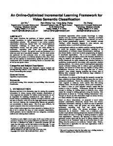
ization. As a result, using an already trained model, we are able to immediately provide accurate link quality estimates based on current measurements, there is no need to build or revise local statistics. Other approaches that deal with fast adaptation to dynamic changes in the network include [26], [27], [28]. A fourth requirement for a good link quality estimator is related to link-asymmetry awareness. In [7], the authors propose an estimator that is able to effectively identify wireless link asymmetry and improve the overall utilization of network capacity. In our approach, we also learn to predict the quality of unidirectional links. We also demonstrate, in Sec. VI, how our estimates can be used to calculate the cost of bi-directional links for the purpose of routing. III. A RCHITECTURE OF THE LQL P ROTOCOL A. System Overview At each node, the LQL protocol, consists of two connected components: a sample collection protocol (Sec. III-C) and a supervised learning module (Sec. III-D). The general LQL architecture is presented in Figure 1, showing the internal and external I/O relationships at a single network node.

B. Local network configuration and feature vector Since we aim to learn a mapping between a local network configuration and the quality of the link associated to the configuration (its PPR in our case), we first identify a set of network features that summarize the local network configuration. We selected features that are both relatively easy (feasible) to measure and clearly represent major factors determining the effective quality of a wireless link. We focus on features that are significant for carrier sense multiple access (CSMA) based MAC protocols. However, our approach can be applied with other MAC protocols, provided that an appropriate set of features is selected. In the following the reasons behind the selection of each feature are briefly discussed. It is widely understood that the PPR between two neighbor nodes is directly related to their physical distance, therefore we included the distance between the two end nodes of the wireless link in the feature set. The Received Signal Strength Indicator (RSSI) is a hardware based-estimator embedded in many wireless devices. It is usually available directly from the PHY layer and is commonly included in link quality prediction models. We also include it, even if its efficacy as a link quality estimator by itself has been disputed in many research works [9]. We also consider the Signal-to-Noise Ratio (SNR), which has also being commonly used as a link quality indicator. It is worth to mention that our experiments (not reported in the paper) showed that it is not needed to use all these three features (distance, RSSI, and SNR) together to achieve high prediction accuracy: only one of them, combined with the other features described below is enough to build a reliable and accurate model. Another feature that we consider is the traffic load at the sender, rS (we are considering directional links, connecting a sender node, S, to a receiver node, R). The rate at which data traffic flows from S to R through the link has a clear impact on the amount of expected packet losses. In a similar way, high traffic load at the receiver can also lead to packet losses (e.g., due to destination busy collisions [29]). Hence, we also consider the transmission rate at the receiver, rR , as relevant network feature. It is clear that, in general, considering traffic generation rates does not take into account the expected effective occupation of the wireless channel from a node, since this also depends on packet sizes, and on the characteristics of the

Fig. 1. Node’s view of the architecture and relationships of the LQL protocol.

The sample collection protocol works concurrently with user applications and other network protocols. Its main tasks consists in calculating the numerical values representing the local network configuration (feature vector, see Sec. III-B) and assessing the corresponding link quality value in terms of estimated PRR. In other words, the sample collection protocol monitors the local network configuration (measuring RSSI, SNR, and other values), and during the time the configuration is stable, the PRR of the link under consideration is measured (see Sec. III-C). When the local configuration changes (e.g., a neighbor has moved away or has changed its traffic generation rate), the pair composed of the feature vector and the measured PRR value is locally stored as a training sample. This is then passed to the supervised learning component of the protocol, which updates its internal statistical link quality predictor model incrementally, after every received sample. It also provides link quality estimates as a cross-layer service to other protocols and applications. While the learning component does its job, the sample collection component starts gathering a new training sample, based on the new local configuration. The whole process is iterated over time at the nodes in a fully distributed way. The training samples are also shared between the nodes, in order to cooperatively enlarge the training set available at a node and speedup the overall learning process. A training 71

2013 12th Annual Mediterranean Ad Hoc Networking Workshop

meantime it calculates the corresponding link quality metric, which in our case is the PRR. Finally, the protocol reacts to changes in the local network configuration: When a change is detected, the current sampled is stored or discarded (depending on whether or not sufficient information was gathered in terms of number of observations), and possibly a new sample is initialized. The protocol that we present here is based on the passive monitoring of incoming and outgoing network traffic at the nodes. Passive monitoring is used for two main objectives: keeping updated the neighbor tables and estimating outgoing traffic rates. At the same time, the information about RSSI and SNR corresponding to a given neighbor is gathered (if it is available), and the number of received packets is updated (for PRR estimation). The outgoing traffic rate of a node is estimated by considering the payload size of all its outgoing packets (and calculating a moving average of this size). However, the passive local monitoring itself is not sufficient to figure out the effective PRR: it is necessary to know what was the effective data generation rate at the sender in order to compute the PRR at the receiver. This information is obtained by means of summary packets, which are broadcast messages sent by every node generating traffic. They are broadcast at a low rate (e.g., once every second), in order to minimize the generated overhead. Summary packets contain information about a sender node’s outgoing transmission rate, neighborhood (in a form of the compact FS vector described in Section III-B), and number of packets transmitted since the last summary packet (in order to better and incrementally estimate the PRR at the receiver). In this way, each node has enough information to build a link quality training sample. However, in order to accept the sample, we require two conditions to be met: the local wireless environment remains stable during the whole sampling period (sample consistency), and a statistically significant assessment of the PRR for the link can be calculated. In order to ensure the statistical significance of the measured PRR, we require that either a sufficient number of packets is received (we used 25 packets in the experiments), or the session lasts for a sufficient period of time (2 seconds in the experiments). The requirement for sample consistency is guaranteed as long as the value of the selected features of the local network configuration remain constant during the entire sampling session. Assuming that, for instance, a node R is collecting measurements of an existing link S → R, two events at R enforce the protocol to perform actions to check the consistency of the current link sampling session and possibly restart it: a change in the neighborhood state of the sender node S (remote environment change), and a variation in the state of the receiver node R (local environment change). The remote environment change event is detected through the information contained in the summary packets transmitted by S. In this case, the sampling session for the link S → R is interrupted, and possibly a new session is started. If the statistical significance requirements are met, the sample is accepted. Otherwise, it is discarded. The local environment change event is triggered at node R when its estimated sending rate changes (detected through passive monitoring), its neighbor table is modified, or the sending rate or RSSI of any of its neighbors changes. The occurrence of a local environment change event implies that the local configuration of all links currently being monitored by R have been modified. Therefore, all sampling sessions

specific MAC contention protocol and of queue management failures, among others. However, hereafter traffic generation rate is used as a feature for expressing in a rather general and compact way the impact of traffic loads on link quality. In wireless networks, interfering transmissions contribute to poor packet delivery performance. To consider this factor in our model, we include receiver’s neighborhood state in the feature set, by considering a vector VR of elements (ni , RSSIi , ri ). In the vector, ni is an active neighbor of the receiver (i.e., a neighbor active in transmitting during the considered time period), which is transmitting with signal strength RSSIi at a packet rate ri . Furthermore, since simultaneous transmissions from nodes in the vicinity of the sender S can also affect link quality, also the sender’s neighborhood state is included in the feature set, following a similar approach as in the case of VR . More precisely, we use as feature the vector VS , which include tuples (nj , RSSIj , rj ) representing a neighbor node nj , transmitting with signal strength RSSIj , at a packet rate rj . Since some of the variables above which have selected as features to represent the local network configuration can take any value over a possibly large range of values, we adopted a coarse-grained representation of their values, which is more amenable to learning. More specifically, we assume that the traffic loads rS and rR belongs to one of three possible traffic profiles in the set Tprof = {rlow , rmed , rhigh }, expressed in terms of selected data rates (e.g., if rlow , rmed , rhigh are respectively 10, 100, and 1000 Kbps, a traffic generation rate rS = 80 Kbps belongs to rmed ). Similarly, also RSSI and SNR values are discretized in three possible profiles respectively RSSIprof = {RSSIlow , RSSImed , RSSIhigh } and SN Rprof = {SN Rlow , SN Rmed , SN Rhigh }. Based on these discretizations, we represent the sets VS and VR in a compact way by grouping their values based on RSSI and traffic rates. In fact, since in VS and VR each RSSIk can only belong to one of the three profiles in RSSIprof , and each traffic rate rk can only belong to one the the three traffic profiles in Tprof , each active node nk can only belong to 1 out of 9 possible joint combinations of RSSI and traffic rate. Therefore, we can represent the sets VS and VR by means respectively of the vectors FS = (FSij , i, j = {low, med, high}) and FR = (FRij , i, j = {low, med, high}), with 9 integer components each. The component of index (i, j) corresponds to the number of neighbors having RSSI = RSSIi and r = rj . For instance, FRmed,low indicates the number of neighbors of the receiver with RSSI = RSSImed and r = rlow . Using this vector representation for the sets VS and VR , we obtain a numerical vector of 23 values, which is used as feature vector to summarize in a compact way the local network configuration: (distance, RSSI, SN R, rS , rR , FS , FR ).

(1)

Each value is normalized in [0, 1], based on the observed minimum and maximum values. The resulting vector is given as input to the LQL learning component, C. On-line sample collection protocol The on-line sample collection component of the LQL protocol deals with multiple tasks. First, for a given wireless link, it keeps measuring and monitoring the values of all the features described in the previous section (Sec. III-B), ensuring that the local network configuration is stable. Second, in the 72

2013 12th Annual Mediterranean Ad Hoc Networking Workshop

collection (i.e., before its use to update the model). We report the mean squared error (MSE) averaged in a moving window (the default window size is 50 seconds). We also report the final MSE value and the boxplot of the distribution of absolute prediction errors, both calculated starting at a certain time after the initial learning phase (after the MSE value stabilizes over time). These results are always averaged over all the nodes taking part in the simulation.

must be restarted and each sample must be verified in terms of its statistical significance. D. Supervised incremental learning In our approach, we use an incremental learning technique. Thus, after a sample is accepted, it is immediately used to update the link quality model. Adopting an incremental approach allows for significant savings in resources, both in terms of memory (there is no need of buffers for storing training samples) and CPU time (only one sample at a time is being processed). The machine learning model that we use for incremental learning is based on the Locally Weighted Projection Regression (LWPR) [12]. LWPR is an incremental regression algorithm that can provide robust non-linear function approximation in high dimensional spaces [30]. To use LWPR in an on-line manner, we had to prior analyze the characteristics of the data and tune some internal parameters. For this purpose, we performed an initial large experiment, collecting a large set of 20,000 samples. From this set we obtained minimum and maximum values for the features, required for their normalization. Next, we also performed feature ranking in order to check feature importance and eliminate the possibly redundant and/or correlated features. We used the well-established feature selection approach of Weka [31], namely the Information Gain for evaluating the worthiness of an attribute in the prediction task based on entropy [20]. We observed that features distance, RSSI and SN R are the most critical ones to differentiate good links from bad ones. However, overall, all features contribute with a significant weight in predicting link quality. Thus, we decided to use all features described in Section III-B to train the regression models. Finally, we tuned the internal parameters of LWPR following the parameter tuning procedure suggested in [32]. The following parameters were adjusted in order to minimize the mean squared error for the set of training data: initial distance metric (initD = 5I), learning rate (initα = 50), penalty factor (penalty = 0.0001), and weight activation threshold (wgen = 0.15). IV.

A. Various topologies In a first set of experiments, we show the evolution of the link quality prediction accuracy of the proposed incremental learning approach, considering various network topologies, composed of 25 up to 250 nodes. When we change the number of nodes, we also adjust the size of the simulation area in order to keep node density constant (e.g., for 250 nodes we have the area of 1900×1900 m2 ). Each node builds its own individual link quality model, without exchanging samples with other nodes. 50 nodes 100 nodes 150 nodes 250 nodes

0.5 0.4 0.3 0.2

1 Absolute deviation

MSE in moving window

0.6

0.8 0.6

MSE: 0.024

MSE: 0.029

MSE: 0.025

MSE: 0.028

MSE: 0.029

100

150

200

250

0.4 0.2

0.1 0 0 0

500

1000 Time [sec]

1500

50

Nodes number

Fig. 2. Evolution of prediction accuracy: window averaged MSE for various topologies (left). Final prediction accuracy: distribution of absolute prediction errors calculated after the 1000th second (right).

We present the selected results on Figure 2. It can be seen that the proposed approach performs well in the different network topologies. In the initial learning phase, when nodes receive first samples and start to train link quality models, prediction errors are high. After a certain time (slightly longer for larger networks), the MSE values converge to a low value. This indicates that a sufficient number of samples were collected, and that the models were trained with enough information to provide accurate link quality estimates. Results show that, after an initial phase, the accuracy of the LWPR model is very good. It can be also seen that during the initial phases errors tend to slightly increase with the increase of network size.

E VALUATION IN SIMULATION : MOBILE AD HOC SCENARIOS

In this section, we present the results of a detailed evaluation of the proposed approach in a simulation environment. Namely, we use the NS-3 network simulator [33] with the following configuration. We simulated 802.11a Wi-Fi networks, with the transmission rate of 6 Mbps. We used a log-distance propagation loss model with default parameters (path loss exponent set to 3.0). This corresponds to a transmission range of roughly 120 m. Although we consider various scenarios, with number of nodes ranging from 25 up to 250, we define a basic scenario as follows (and we use it, unless stated otherwise). We place 50 nodes on the area of 850× 850 m2 , and we use a common Random Waypoint mobility model with a speed of 1 m/s and a pause time of 20 seconds. Each node generates a constant bit rate (CBR) traffic in a form of 1-hop broadcast transmissions, with one of the three possible rates: 1.5 Mbps, 400 Kbps or 80 Kbps (assigned randomly). Packet size is set to 1000 bytes. We run simulations for 3000 seconds and we measure prediction errors, i.e., the difference between measured and predicted values of the packet reception rate. The prediction error is calculated for each sample immediately after its

B. Information exchange The second set of experiments investigates the influence of information sharing on the learning performance. Nodes either build their link quality models individually, based on the samples they collected themselves, or they exchange the collected samples within the N -hop neighborhood. In Figure 3, we consider 1-hop and 2-hop neighborhoods. In order to emphasize the difference, we make collecting the samples more difficult, by increasing node speeds to 5 m/s. The results show that information exchanges between the nodes can significantly speedup the learning process. This is in line with the expectations: due to the extended number and diversity of samples, every node has a better regression model that is more prepared to describe already known local configurations and to face previously unseen configurations. 73

2013 12th Annual Mediterranean Ad Hoc Networking Workshop

D. Overhead analysis In this section, we focus on the communication overhead of the proposed approach. Without sample sharing mechanism, our protocol generates only periodical summary messages (in our case, once per second in each node). Moreover, the information from summary packets could be possibly added to into the packets generated by other protocols, such as periodic HELLO messages which are commonly used in many routing protocols. The number of packets generated with active sample sharing depends on the topology, the selected number of hops to relay the message, and on the number of samples which have collected. Sample results regarding overhead are shown in Figure 5 (left). It can be seen that overall the protocol generates a relatively small overhead, which is not expected to cause a significant impact on user traffic. The results presented in Figure 5 (right) confirm this: at each node, the average number of received data packets only drops only 2% in the worst case, compared to the case without the LQL protocol running.

0.03 0.02 0.01

0.8

500

1000 1500 2000 Time [sec]

2500

3000

0,5 0

25 nodes 50 nodes 75 nodes 100 nodes 0,99 0,98 0,98 0,98

0,99 0,99 0,99 0,99

0,99

1,00 1,00 1,00 0,99

1,00 1,00 1,00 1,00

Averaged received data ratio

1

2,8

Packets sent (per sec. per node)

MSE: 0.048

MSE: 0.009

0.2

wmewmaPRR

2 1,5

1

0,98 0,97

0,96 No LQE

No sharing 1 hop 2 hop Link Quality Estimation mode

We also analyzed the computational performance of LQL. We skip detailed results here due to the space constraints. Nevertheless, the results confirmed that the incremental learning approach allows for significant savings in computational resources. On a typical PC machine, updating a LWPR model (which was previously trained on 1000 samples) with a single sample consumes no more than 0.02 of a millisecond of the CPU time. A single prediction operation on the same model consumes on average 0.02 ms as well. While training a model with 1000 samples, the maximum measured memory usage did not exceed 400 kB. The processing required to build samples is also relatively cheap: it contains only simple operations (such as averaging, discretization, and normalization) and can be performed only when the environment change is detected (see Sec. III-C).

0 0 0

2,5

1,01

Fig. 5. Communication overhead (default scenario). The number of the overhead packets generated per node per second (left) and the influence on the ratio of correctly received vs. generated data packets (right).

0.6 0.4

3

25 nodes 50 nodes 75 nodes 100 nodes

No sharing 1 hop 2 hops Link Quality Estimation mode

1

wmewmaPRR LWPR 0.04

Absolute deviation

MSE in moving window

0.05

4 3,5

3,7

C. Comparison with other link quality estimators In this section, we compare our approach with other link quality estimators. Referring to the comprehensive survey in [9], we have initially chosen for comparison two hardwarebased estimators (based on averaged RSSI and SNR) and one software-based estimator (wmewmaPRR which is the Window Mean with Exponentially Weighted Moving Average estimator based on the filtered packet reception rate value [23]). Our preliminary experiments confirmed the observations made in [9]: both hardware based estimators were only capable of distinguishing between very good and very bad links. On the other hand, both the wmewmaPRR estimator and our approach were able to provide accurate estimates for links of different quality levels. Thus, we performed a further experiment in order to compare our model and the wmewmaPRR estimator in a highly dynamic scenario. We set the nodes speed to infinity, and we define a random pause time within a range of [5.0 − 10.0] seconds. In this fashion, a node moves instantly without affecting the local configurations of the nodes passed along its way. As a result, we have dynamic topology changes together with the desired periods of stability (resulting from pause times) that are required in order to assess the actual PRR with statistical significance (and calculate prediction errors). For wmewmaPRR, we set the window size to 0.5 secs and the smoothing factor α = 0.6, as suggested in [23].

3,1

Fig. 3. Evolution of prediction accuracy for different modes of information sharing: no sharing, 1-hop, and 2-hops sharing. Nodes’ speed is set to 5 m/s.

2,7

1000

1,5

800

1,7

400 600 Time [sec]

1,7

200

1,5

0 0

1,0

0.2

1,0

0.4

1,0

No sharing 1−hop sharing 2−hop sharing

0.6

1,0

MSE in moving window

0.8

LWPR

Model name

V.

Fig. 4. Comparison of estimators under a highly dynamic scenario (high speed, pause time 5.0-10.0 secs). Moving MSE (left) and distributions of the absolute error calculated since the 1000th second (right).

R EAL - WORLD VALIDATION :

A DYNAMIC SENSOR NETWORK SCENARIO

In order to further validate the results obtained in simulation, we evaluated the prediction accuracy of our approach through real-world experiments. We used the INDRIYA Testbed [14] composed of 139 sensor motes with an indoor range of approximately 20 to 30 meters. Considering limited computational capabilities of the sensor motes, we used the testbed in order to collect detailed data (including samples, their timestamps and the corresponding logical node IDs, as well as some topological information, overhead information, etc.), and then we simulated the online learning process on a desktop machine. Due to the fact that the sensor nodes in the INDRIYA network are static, and in order to maximize the number of

The results on Figure 4 show that indeed our approach performs better in the dynamic environment. Although wmewmaPRR performs better at the beginning, it is outranked by our models after the initial learning phase. This demonstrates fast adaptation capabilities of the proposed approach: our trained models can provide immediate estimates based on current measurements, while software-based estimators such as wmewmaPRR require some time to gather sufficient statistics in order to adapt their current assessments. This property can be very beneficial in many applications, such as routing in mobile networks (see Section VI). 74

2013 12th Annual Mediterranean Ad Hoc Networking Workshop

link between a and b in terms of the Expected Transmissions Count (ETX). The cost of a path which is composed of many wireless links is simply calculated as the sum of costs of the individual links. OLSRd therefore, makes use of ETX instead of the number of hops as routing metric for calculating shortest paths. Here we follow a similar procedure, replacing the simple link quality estimates for defining the ETX metric withe the ones provided by our link quality model. In what follows, we refer to our implementation as to OLSR-LQE. We performed a set of experiments in multi-hop routing scenarios, considering the same network configurations as the ones described in Section IV. Data traffic is generated by 10 CBR sources, sending data to 10 randomly chosen destinations at the rate of 96 Kbps. We compared the average throughput achieved by three routing algorithms: OLSR, OLSRd (with quality extensions), and OLSR-LQE. Since in this case we are not interested in the incremental performance, we first used the LQL protocol to train the link quality prediction model using 20,000 samples collected in a network composed of 50 nodes, and then installed the trained model on the OLSR-LQE nodes.

0.8

0.6 Absolute deviation

0.5 0.4 0.3 0.2

0.6

MSE: 0.021

0.4 0.2

45

0

40

0.1 0 0

500

1000 Time [sec]

1500

Throughput [Kbps]

MSE in moving window

0.7

LWPR Model name

Fig. 6. Results for the INDRIYA testbed comprised of 139 wireless sensor motes. Moving MSE (left) and distributions of the absolute error (right).

35 30 25 20 15 25

The results (Figure 6) are in line with corresponding simulation results from Section IV. The learning curves for both incremental and batch approaches are very similar to the ones obtained in simulation: the learning time is comparable with our default scenario, and the final accuracy is even better than in the case of simulation. Thus, our approach was able to provide very accurate link quality predictions in the real wireless environment, proving its usability and robustness to noisy conditions.

OLSR OLSRd OLSR−LQE

50 75 Number of nodes

100

25 Throughput [Kbps]

observed topologies, the experiments were designed considering sub-networks of 40 logical nodes each, sampled out of the 139 physical nodes of the full INDRIYA network. The nodes in each sub-network have been randomly selected, with the condition that each node has at least one neighbor. Each sub-network operates for 3 minutes. After that, a new subnetwork is selected, simulating in this way network changes related to mobility and/or node failures. Individual nodes also change their data generation rates (at the application layer). Rate changes occurred with intervals uniformly distributed between 5 and 45 seconds. The selected data rates are also uniformly distributed between 5 and 35 packets per second. Data packet size is set to 100 bytes. Considering the information provided by the testbed, we used the following feature vector: (RSSI, rS , rR , FS , FR ) (see Sec. III-B).

OLSR OLSRd OLSR−LQE

20 15 10 5 0 1

2

3 Speed [m/s]

4

5

Fig. 7. Comparison of the original OLSR, OLSR with simple link quality extensions (OLSRd), and OLSR employing the LQL estimator (OLSRS-LQE). Average throughput vs. number of nodes (left) and vs. node speed (right). Results are averaged over 20 simulations.

In the first set of experiments (Figure 7, left), we consider the effect of increasing the number of nodes in the network under relatively slow dynamics (nodes speed of 1 m/s). It can be observed that both algorithms using link quality estimates perform better than the original OLSR. The difference increases with the increase of the network size: in larger networks, the average number of hops required to reach a destination is higher, thus choosing better wireless links becomes more important for performance, such that bot OLSRd and OLSR-LQE shows an increasingly better performance compared to the basic OLSR. OLSR-LQE shows the better overall performance. In the 100-nodes network OLSR-LQE offers a roughly 40% increase of throughput in comparison to the original OLSR algorithm. In the second set of experiments (Figure 7, right), we increase the dynamics of topology changes by varying nodes’ speed from 1 to 5 m/s. We can see that while OLSR-LQE still shows its benefits over OLSR, the performance of OLSRd rapidly deteriorates in highly mobile networks. This can be the effect of the poor reactivity of the simple link quality estimator used by OLSRd. As OLSRd actually employs a software-based PRR estimator, this behavior is in line with the results of our previous experiments from Section IV-C. Another observations is that the advantages of OLSR-LQE over OLSR are lower in highly mobile environments. This agrees with the intuition that under frequent topology changes, the main cause of packet losses is the lack of routing information, and not really how imprecise or imprecise is the routing metric. In general, it is

VI. A PPLICATION TO ROUTING IN MANET S In this section, we show how the reliable link quality estimates provided by LQL can be directly applied to improve the overall performance of the Optimized Link State Routing Protocol (OLSR) [15] for mobile ad hoc networks (MANETs). OLSR is one of the main standards for mobile ad-hoc and mesh networks, and is based on the typical link-state approach in which the network topology database is maintained synchronized across the network. For calculating a routing table, Using routing table information, the reference version of OLSR assigns routes based on shortest path calculations minimizing the number of hops between source-destination pairs. Implementations such as the open source OLSRd [34] (commonly used on Linux-based mesh routers) extends this basic hop-based metric by relying on some simple link quality sensing. Hereafter, we show that replacing the simple link quality estimator employed in the OLSRd implementation with our link quality model significantly improves the routing performance of the protocol. In OLSRd, the quality of a wireless link between two nodes a and b corresponds to the probability of receiving in b a packet sent from a. This is estimated in a rather basic way using periodical HELLO messages. For instance, if 2 out of 10 packets are lost on their way from b to a, the probability is set to 0.8. This probability is used to calculate the cost of the 75

2013 12th Annual Mediterranean Ad Hoc Networking Workshop

well understood that a proactive protocol as OLSR might not be suitable to deal with highly dynamic scenarios.

[13]

VII. C ONCLUSIONS AND FUTURE WORK We proposed LQL, a protocol for the on-line supervised incremental learning of link quality estimates in wireless networks, both static and mobile. The protocol mainly rely on the passive overhearing of local traffic, and generates little local overhead. It also provides a simple yet effective way to let the nodes sharing locally gathered training samples and performing a cooperative form of learning, which speedups nodes’ learning and adaptation. We have shown, both in simulation and using a real testbed, that LQL can provide fast and reliable link quality estimates, even when highly dynamic mobile networks are considered. The use We compared LQL with existing state-of-the-art link quality estimators, showing the advantages of using a trained model versus estimators that need to gather and process statistical data on the fly. Many directions of future work can be envisaged. We plan to apply the proposed scheme for improving multi-hop communications in networked mobile robots. In particular, we plan to exploit controlled robot mobility in order to dynamically reshape network topology selecting the most reliable local network configurations. We also aim to extend the estimator with the capability of assessing the stability of the link and to work with different, composite quality metrics.

[14]

[15]

[16]

[17]

[18]

[19]

[20]

[21]

ACKNOWLEDGMENTS This research has been partially funded by the Swiss National Science Foundation (SNSF) Sinergia project SWARMIX, project number CRSI22 133059.

[22] [23]

R EFERENCES [1]

[2]

[3]

[4]

[5]

[6]

[7]

[8]

[9]

[10]

[11] [12]

D. S. J. De Couto, D. Aguayo, J. Bicket, and R. Morris, “A highthroughput path metric for multi-hop wireless routing,” in Proc. of MobiCom ’03, pp. 134–146, ACM Press, 2003. R. Draves, J. Padhye, and B. Zill, “Routing in multi-radio, multi-hop wireless mesh networks,” in Proceedings of MobiCom, pp. 114–128, ACM Press, 2004. A. Krause, C. Guestrin, A. Gupta, and J. Kleinberg, “Near-optimal sensor placements: Maximizing information while minimizing communication cost,” in Proc. of IPSN’06, pp. 2–10, ACM, 2006. R. Wattenhofer and a. Zollinger, “XTC: A practical topology control algorithm for ad-hoc networks,” Proc. of the 18th International Parallel and Distributed Processing Symposium, pp. 216–223, 2004. Y. Yang, J. Wang, and R. Kravets, “Interference-aware load balancing for multihop wireless networks,” Tech. Rep. 361702, University of Illinois at Urbana-Champaign, 2005. E. Feo and G. A. Di Caro, “A flow-based optimization model for throughput-oriented relay node placement in wireless sensor networks,” in Proc. of the 28th ACM Symp. on Applied Computing (SAC), 2013. K.-H. Kim and K. G. Shin, “On accurate and asymmetry-aware measurement of link quality in wireless mesh networks,” IEEE/ACM Transactions on Networking, vol. 17, no. 4, pp. 1172–1185, 2009. T. Melodia, D. Pompili, and I. Akyildiz, “A communication architecture for mobile wireless sensor and actor networks,” in Proc. of IEEE SECON’06, pp. 109–118, IEEE, 2006. N. Baccour, A. Koubˆaa, M. Zuniga, H. Youssef, C. Boano, and M. Alves, “Radio link quality estimation in wireless sensor networks: a survey,” ACM Transactions on Sensor Networks, vol. 8, no. 4, 2012. V. Kolar, S. Razak, P. M¨aho¨onen, and N. B. Abu-Ghazaleh, “Link quality analysis and measurement in wireless mesh networks,” Ad Hoc Networks, vol. 9, no. 8, pp. 1430–1447, 2011. C. Renner, S. Ernst, and C. Weyer, “Prediction accuracy of link-quality estimators,” in Proc. of EWSN’11, 2011. S. Vijayakumar, A. D’souza, and S. Schaal, “Incremental online learning in high dimensions,” Neural Comp., vol. 17, pp. 2602–2634, 2005.

[24]

[25]

[26]

[27]

[28]

[29]

[30] [31]

76

E. F. Flushing, J. Nagi, and G. Di Caro, “A mobility-assisted protocol for supervised learning of link quality estimates in wireless networks,” in Proceedings of the Int. Conf. on Computing, Networking and Communications (ICNC), International Workshop on Mobility and Communication for Cooperation and Coordination (MC 3 ), 2012. M. Doddavenkatappa, M. C. Chan, and A. L. Ananda, “Indriya: A low-cost, 3d wireless sensor network testbed,” in Proceedings of the TRIDENTCOM, pp. 302–316, 2011. P. Jacquet, P. Muhlethaler, T. Clausen, A. Laouiti, A. Qayyum, and L. Viennot, “Optimized link state routing protocol for ad hoc networks,” in Proc. of the IEEE Int. Multi Topic Conf. Technology for the 21st Century (INMIC), pp. 62–68, 2001. H. Zhang, A. Arora, and P. Sinha, “Link estimation and routing in sensor network backbones: Beacon-based or data-driven?,” IEEE Trans. on Mobile Computing, vol. 8, no. 5, pp. 653–667, 2009. G. Judd, X. Wang, and P. Steenkiste, “Efficient channel-aware rate adaptation in dynamic environments,” in Proc. of MobiSys, pp. 118– 131, ACM Press, 2008. S. H. Shah, K. Chen, and K. Nahrstedt, “Available bandwidth estimation in IEEE 802.11-based wireless networks,” in Proc. of 1st ISMA/CAIDA Workshop on Bandwidth Estimation, 2003. K. Farkas, T. Hossmann, F. Legendre, B. Plattner, and S. Das, “Link quality prediction in mesh networks,” Computer Communications, vol. 31, pp. 1497–1512, may 2008. Y. Wang, M. Martonosi, and L.-S. Peh, “Predicting link quality using supervised learning in wireless sensor networks,” ACM SIGMOBILE Mobile Computing and Communications Review, vol. 11, no. 3, pp. 71– 83, 2007. N. Baccour, A. Koubˆaa, H. Youssef, M. Ben Jamˆaa, D. do Ros´ario, M. Alves, and L. Becker, “F-LQE: A fuzzy link quality estimator for wireless sensor networks,” in Proc. of 7th European Conference on Wireless Sensor Networks, pp. 240–255, 2010. T. Liu and A. E. Cerpa, “Foresee (4C): Wireless link prediction using link features,” in Proc. of IPSN’11, pp. 294–305, 2011. A. Woo and D. Culler, “Evaluation of efficient link reliability estimators for low-power wireless networks,” tech. rep., EECS Department, University of California, Berkeley, 2003. M. Senel, K. Chintalapudi, D. Lal, A. Keshavarzian, and E. Coyle, “A kalman filter based link quality estimation scheme for wireless sensor networks,” in Global Telecommunications Conference, 2007. GLOBECOM ’07. IEEE, pp. 875 –880, 2007. R. Fonseca, O. Gnawali, K. Jamieson, and P. Levis, “Four-Bit wireless link estimation,” in Proc. of the Sixth Workshop on Hot Topics in Networks (HotNets), 2007. A. Becher, O. Landsiedel, G. Kunz, and K. Wehrle, “Towards short-term wireless link quality estimation,” in Proc. of the 5th ACM Workshop on Embedded Networked Sensors, (Chalottesville, Virginia), 2008. M. H. Alizai, H. Wirtz, G. Kunz, B. Grap, and K. Wehrle, “Efficient online estimation of bursty wireless links,” in Proc. of the 16th IEEE Symp. on Computers and Communications (ISCC), pp. 191–198, 2011. C. A. Boano, M. A. Z. Zamalloa, T. Voigt, A. Willig, and K. R¨omer, “The triangle metric: Fast link quality estimation for mobile wireless sensor networks,” in Proc. of the 19th Int. Conference on Computer Communications and Networks (ICCCN), pp. 1–7, 2010. A. Nasipuri, J. Zhuang, and S. Das, “A multichannel CSMA MAC protocol for multihop wireless networks,” in Proc. of IEEE WCNC’99, vol. 3, pp. 1402–1406, 2002. C. Atkeson, A. Moore, and S. Schaal, “Locally weighted learning,” Artificial Intelligence Review, vol. 11, pp. 11–73, 1997. M. Hall, E. Frank, G. Holmes, B. Pfahringer, P. Reutemann, and I. Witten, “The WEKA data mining software: an update,” ACM SIGKDD Explorations Newsletter, vol. 11, no. 1, pp. 10–18, 2009.

[32]

S. Vijayakumar and S. Klanke, “A library for Locally Weighted Projection Regression - Supplementary documentation.” http://wcms.inf.ed.ac.uk/ipab/slmc/research.

[33]

NS-3, “Discrete-event network simulator for Internet systems.” http://www.nsnam.org.

[34]

OLSRd, “An adhoc wireless http://www.olsr.org.

mesh

routing

daemon.”