Only Mostly Blind Source Separation Using Source Hypotheses to Augment Blind Source Separation Richard Goldhor Keith Gilbert Joel MacAuslan Speech Technology & Applied Research Corp. Bedford, MA
[email protected]
Karen Payton Electrical & Computer Engineering Department University of Massachusetts, Dartmouth North Dartmouth, MA Abstract—In acoustic and bioelectrical environments characterized by multiple simultaneous sources, effective blind source separation from sensor response mixtures becomes difficult as the number of sources increases—especially when the true number of sources is both unknown and changing over time. However, in some environments, non-sensor information can provide useful hypotheses for some sources. Focusing for convenience on the acoustic case, we propose an adaptive filtering architecture for validating such hypotheses, extracting an acoustic representation of valid hypotheses, and improving the separation of the remaining “hidden” acoustic sources. We evaluate the performance of this “Only Mostly Blind Source Separation” algorithm on synthesized instantaneous (bioelectrical-like), synthesized non-instantaneous, and true convolutive acoustic mixtures of simultaneous speech material. Keywords-BSS, blind source separation, hypothesis validation, signal extraction.
I.
INTRODUCTION
Many acoustic and bioelectrical environments comprise multiple simultaneously active sources, and the responses of sensors placed in those environments consist of convolutive mixtures of those source signals. The problem of recovering the “hidden” (unknown) source signals from the mixtures alone is known as blind source separation (BSS). A variety of BSS algorithms have been proposed [1, 2, 3, 4]. Reference [3] describes a particularly efficient and flexible algorithm with good temporal stability. This algorithm, hereinafter called “ABYK”, is used as the core of the BSS processing described in this paper. For convenience but without loss of generality, in this paper we focus primarily on the acoustic situation. To completely separate N simultaneous sources, ABYK, like many other BSS algorithms, must have available at least N linearly independent mixtures (microphone inputs). In realworld situations this may represent a significant restriction on practical use. Not only is the number of simultaneous sources typically changing from moment to moment—often the actual count is unknown. Furthermore, it is usually impractical to This research was partially supported by NIH Grants R43DC006379, R43DC011668, and R43DC011475.
dynamically add additional physical microphones whenever a new source becomes active. However, in many practical scenarios non-acoustic information may be available about one or more of the acoustic sources. For instance, in an airport gate area, a TV news feed is often a prominent source in the acoustic environment. Another source, active from time to time, may generate pre-recorded security announcements. In both of these cases, and in many similar ones, electronic signals drive loudspeakers that constitute significant acoustic sources in the environment. These electronic driving signals constitute non-acoustic information related by an unknown transfer function to the acoustic radiation from loudspeakers that would contribute to the responses of microphones in that environment. These examples represent a subset of the more general situation in which prior information is available to guide our inference of the constituent sources that comprise the acoustic mixtures [5]. In this paper, a source for which non-acoustic information is available is called a traceable source, and a signal which may constitute such non-acoustic information is called a source hypothesis. An acoustic source for which no source hypothesis is available is called a hidden source. A source hypothesis is considered valid if it does in fact correspond to a currently active acoustic source. Otherwise, the source hypothesis is deemed to be invalid. Source hypotheses have the advantage over sensor responses of being pure: that is, not being mixed with other sources. Furthermore, we require that they be statistically independent of each other. We have been investigating the use of source hypotheses as a way to improve the performance of source separation algorithms. When properly exploited, both microphone responses and source hypotheses may contribute to effective source separation. Microphone responses are always valid, but are often not pure; source hypotheses are always pure (by definition), but are not always valid. We hope to show that a valid source hypothesis can be at least as effective as an additional physical microphone in supporting source separation. At the highest level, our strategy is to 1) determine the validity of a source hypothesis; 2) estimate the traceable
978-1-4673-0372-9/11/$26.00 ©2011 IEEE
A: SHVI
B: TSVI
xP
xP sQ
BSS
yP tR uQ-R
sQ
C: SCRUB
BSS
H
tR
yP tR
xP
uQ-R
sQ
P
BSS
yP
tR uQ-R
H
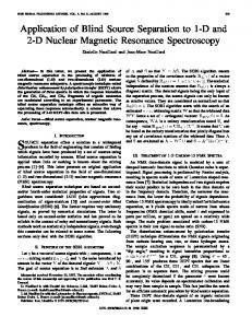
Figure 1: Data flow diagrams corresponding to three OMBSS algorithms (see text). xP is the set of P microphone inputs, sQ is the set of Q source hypotheses, yP is the set of P hidden source estimates, tR is the set of R traceable source estimates corresponding to the R valid hypotheses, and uQ-R is the set of Q-R invalid hypotheses. source corresponding to the hypothesis; and 3) use the traceable source estimate to improve overall source separation. Because we use non-acoustic information to separate both the traceable and hidden sources, we refer to the overall procedure as “Only Mostly Blind Source Separation”, or OMBSS. II.
CANDIDATE OMBSS ARCHITECTURES
When augmenting “completely blind” BSS algorithms with source hypothesis information, two fundamental signal processing decisions must be made. The first decision is whether or not to pre-estimate traceable sources prior to BSS processing, or to depend on a (possibly-modified) version of the core BSS algorithm to generate such estimates. The second decision (which only arises if the first decision is made to preestimate traceable sources prior to performing BSS) is whether or not to “scrub” (remove) those estimated traceable sources from mixture signals before attempting blind source separation, or to depend on the BSS algorithm (again possibly modified) to separate both traceable and hidden sources. Fig. 1 sketches the top-level architectures that correspond to the possible design decisions. The first possibility, a source hypothesis virtual input (SHVI) architecture, is sketched in Fig. 1A. This architecture directly introduces the entire set of Q unvalidated source hypotheses as virtual BSS inputs. It depends on the BSS algorithm to extract and separate both traceable and hidden sources from the P unadulterated microphone mixtures. The disadvantages of this architecture are that it greatly expands the dimensionality of the BSS processing, and it potentially introduces a multiplicity of invalid source hypotheses as virtual inputs with which the BSS algorithm must contend. The second architecture, a traceable source virtual input (TSVI) architecture, is shown in Fig. 1B. This scheme employs an adaptive preprocessor (discussed below) to identify the R valid hypotheses that are actually present in the P input mixtures (xP), out of the Q hypotheses presented (sQ). For each valid hypothesis, a traceable source estimate is constructed and the R traceable sources (tR) are introduced as virtual inputs to the BSS algorithm. This architecture avoids introducing invalid hypotheses into the BSS processing, but, like the previous architecture, increases the dimensionality of the core source separation problem.
The final possible architecture, a source hypothesis prescrubbing (SCRUB) architecture, is shown in Fig. 1C. In the SCRUB architecture, like the TSVI architecture, traceable source estimates are formed prior to attempting blind source separation. Furthermore, all traceable source estimates (tR) are scrubbed from the input mixtures before those mixtures are processed by BSS. The BSS algorithm is only used to separate the hidden sources. A. Source Hypothesis Pre-scrubbing (“SCRUB”) In this paper, we focus on the properties and performance of the SCRUB method of OMBSS. This algorithm uses adaptive preprocessing to identify valid source hypotheses, and to scrub them out of the mixtures (microphone responses) by subtracting the contribution of each traceable source estimate (tR in Fig. 1) from the acoustic mixtures (xP) before those mixtures are input to the BSS algorithm. In the SCRUB algorithm, the BSS processing is unmodified, and the number of inputs to, and outputs from, the BSS algorithm equals the number of mixtures (microphones) available. The adaptive preprocessing algorithm generates, and produces as output, a single traceable source estimate corresponding to each valid source hypothesis, and explicitly identifies invalid hypotheses. B. Adaptive Preprocessing A key element in OMBSS variations that perform adaptive preprocessing is the inclusion of a least mean-squared-error (LMS) module [6]. A block diagram of the LMS module is
x1 s1 —
Σ
+
+
sq Hypothesis Validator
sQ xP —
Σ
+
+
Figure 2: LMS Adaptive Preprocessing
tq or
ur
shown in Fig. 2. The signals s1 through sQ are the library of Q electronic source hypotheses. Signals x1 through xp represent the acoustic mixtures. The algorithm iteratively adjusts estimated filters ĥ11 through ĥQP to minimize the correlations of s1 through sQ respectively with the LMS outputs through (The iterative adjustment is indicated by the blue dashed lines in the block diagram.) This minimization is performed independently for each mixture, and implicitly assumes a linear relationship between each electronic source hypothesis and its corresponding traceable acoustic source. The filters estimate this linear relationship for each hypothesis-mixture pair. By subtracting the sum of filtered hypotheses from xp, the resulting LMS output, , has been scrubbed of any hypothesized sources found to be present in the mixture. It is these scrubbed inputs that are processed by the BSS algorithm. The SCRUB algorithm also uses the filtered versions of the valid hypothesized sources to construct a set of traceable source estimates t1 through tR. But if the energy in a particular hypothesis-mixture filter estimate falls below a threshold set by the algorithm, the corresponding source is considered not to contribute to the given mixture. Each traceable source— corresponding to a valid hypothesis—is estimated from the outputs of filters for that hypothesis having energies above this threshold. These estimates form the SCRUB output vector tR of traceable source estimates. If a particular hypothesis does not A
contribute to any mixture, it is invalid, and becomes a member of the SCRUB output vector uQ-R of invalid source hypotheses. The algorithm is implemented on a block-by-block basis. Since the hypothesized sources could appear at any time in the mixture, and with an arbitrary delay, a preliminary temporal lag adjustment is made over the block length. A cross-correlation is performed between the source hypothesis and the mixture over the block being analyzed. The lag at which the maximum correlation is obtained is used as the preliminary temporal alignment. When the estimated filter coefficients are computed, the lag for each source hypothesis is fine-tuned to match its acoustic correlate in the mixture. III.
MEASURING PERFORMANCE
In the presentation below, we will have occasion to compare two representations of what may (or may not) be intended to be the same signal. A variety of techniques have been proposed for measuring source separation performance [7]. We will use as our similarity metric a nonnegative scalar value, “R”, defined as the peak of the absolute value of the cross correlation between the last ten seconds of the two (100second) signals being compared, with a maximum cross correlation lag of 4096 samples (approximately 250 msecs). In the discussion section, we identify some limitations to this metric, and identify criteria for an improved measure. B
1
0.5
Rsx
R
ss
1
0.5 0
0 1
2
1 3
4
source
1
3
2
2
4
1
mixture
3
2
4
source
source
D
1
1
0.5
0.5
Rsx
Rsx
C
0
0 4
1
3
2 mixture
1
2 source
1 2 mixture
1
2
3
4
source
Figure 3: Sources & mixtures: in each panel, Source 1 (yellow) is JFK, Source 2 (red) is JAS, Source 3 is KDG (green), and Source 4 (blue) is GWN. The height of each column shows the similarity between two signals, as quantified by the performance measure R. Panel A shows the similarity between the four electronic sources—they are nearly perfectly uncorrelated; B shows the composition of the two instantaneous synthesized mixtures (analogous to the bioelectrical case); C the composition of the non-instantaneous mixtures; and D the composition of the acoustic mixtures. In Panels A, B and C, the electronic sources are used to calculate the R values; in D the acoustic sources are used.
IV.
OMBSS EVALUATION PROCEDURE
To test the performance of the SCRUB algorithm, we used three audio recordings as source material. The first source (“JFK”) was a recording of President Kennedy’s inauguration speech. The second source (“JAS”) was a recording of an adult female talker reading text from a magazine article. The third source (“KDG”) was a recording of an adult male talker reading other material. We also created a Gaussian white noise sequence (“GWN”) for use as an invalid source hypothesis. Each source was edited for length to approximately 100 seconds. These recordings are collectively referred to below as the electronic sources. The R values between all pairs of electronic sources were calculated and are shown in Fig. 3A. Two pairs of synthesized mixtures were created from JFK, JAS, and KDG. In the first pair, instantaneous mixtures were created (analogous to bioelectrical signals). The R values between each mixture and the four electronic sources are shown in Fig. 3B. The second pair of synthesized mixtures comprise non-instantaneous (i.e., delayed) mixtures of the three source signals. The R values between those mixtures and the electronic sources are shown in Fig. 3C. Finally, a pair of acoustic mixtures was generated by placing three loudspeakers in a prepared acoustic environment, and playing back all three sources, one source per speaker. The resulting acoustic mixtures are both non-trivially convolutive. The acoustic environment was prepared by locating three loudspeakers at three of the vertices of a 1 meter square within a sound-treated room. Each electronic source was played through a separate speaker. A microphone was placed at the center of the square, and recordings were made of each electronic source played in isolation. These recordings are collectively referred to below as the acoustic sources. Fig. 4 shows the degree of correlation between the electronic and acoustic versions of each source. Because of high-pass filtering in the output electronics, the acoustic sources are not perfectly correlated with the electronic sources.
Rea
0.5
0 1
2
3 electronic 4 source
C
0.5
0.5
Rsy
0.5
0
0
output
1
2
3 source
4
acoustic source
To evaluate the performance of the SCRUB OMBSS algorithm, the electronic version of KDG was used as a valid source hypothesis. The electronic version of GWN was used as an invalid source hypothesis. The two input mixtures in each pair, and two source hypotheses, were processed by the SCRUB algorithm, and R values between the corresponding electronic or acoustic sources and the scrubbed mixtures were calculated,
1
2
4
All three mixture pairs were processed using the unmodified ABYK algorithm. R values between the two ABYK output channels and each of the corresponding sources (electronic or acoustic) were calculated, and are presented in Fig. 5.
1
1
3
The responses of the two microphones were digitally recorded. The R values between each microphone response mixture and the acoustic sources are shown in Fig. 3D.
1
0
1
2
Figure 4: Similarity of electronic and acoustic sources. The identity of the sources is as described in Fig. 3. To create the pair of acoustic mixtures, the three electronic sources were simultaneously played back through their separate speakers. The resulting sound field was sampled by two microphones placed in different locations in the sound field. One was located at the fourth vertex of the square defined by the three loudspeakers. The other microphone was above and to one side of that square: approximately 1.6 m from the two further speakers, and 0.85 m from the closest speaker, and the other microphone.
B
Rsy
Rsy
A
1
1
4 2
output
2 1
3 source
1
3
2 output
1
4
2 source
Figure 5: Performance of ABYK algorithm processing pairs of mixtures of three sources each. Each panel shows the similarity of the two ABYK output channels to each of the four sources. In each panel, Source 1 (yellow) is JFK, Source 2 (red) is JAS, Source 3 (green) is KDG, and Source 4 (blue) is GWN. Panel A shows the results of processing the instantaneous synthesized mixtures; B shows the results for the non-instantaneous mixtures; and C shows the acoustic results. In every case, at least one of the two output channels must, and does, contain more than one of the three source signals. The acoustic R values (Panel C) were calculated with reference to the acoustic sources.
B
C 1
1
0.5
0.5
0.5
0
Rsx
1 Rsx
Rsx
A
0
0 1
4
3
2
2 source
1
mixture
1
4
3
2
2 source
1
mixture
1
4
3
2
2 source
1
mixture
Figure 6: Source hypothesis scrubbing: Each panel shows the similarity of the scrubbed mixtures to their constituent sources. The source identities and versions are as described in Fig. 5. Panel A shows the results of scrubbing the instantaneous synthesized mixtures; B shows the scrubbed non-instantaneous mixtures; and C shows the scrubbed acoustic mixtures. The acoustic R values (Panel C) are calculated using the acoustic sources. In all cases the traceable source (KDG) was effectively removed from all mixtures. as a measure of how well the source hypotheses were scrubbed from those mixtures. The results are presented in Fig. 6. The scrubbed mixtures were then processed by ABYK, and R values were calculated between the mixture sources (electronic or acoustic) and the separated outputs: two hidden and one traceable. The R values for all source-output pairs are presented in Fig. 7. V.
RESULTS
As evident from Fig. 3A, the four electronic sources are uncorrelated with each other. The fourth source, GWN, is never in fact a component in any of the test mixtures. Hence the zero-valued “Source 4” cells in Fig. 3, Panels B, C, and D. It is also evident that the two mixtures in each test pair represent different combinations of the first three sources, and that the instantaneous and non-instantaneous mixing magnitudes are identical. Fig. 4 shows that the acoustic version of each source is not identical to its electronic version. Because the acoustic and
Fig. 5 demonstrates the performance of the “completely blind” ABYK algorithm, absent any assistance from source hypotheses. With the instantaneous simulated mixture, Sources 1 and 2 are separated at the outputs but Source 3 is split, some in Output 1 and some in Output 2. For the simulated delayed mixture, Source 1 is fairly well isolated in Output 1 while Sources 2 and 3 are both strong in Output 2. When the sources are presented acoustically, Source 3 appears at reduced strength in Output 1, mixed with Source 1, while Source 2 appears primarily in Output 2. Fig. 6 shows that the LMS algorithm described above can, in fact, effectively scrub source hypotheses from both instantaneous and convolutive mixtures. Note that in Panel C the actual acoustic source is a filtered version of the
B
C 1
1
0.5
0.5
0.5
0
Rsy
1
Rsy
Rsy
A
electronic versions of sources differ, and the source hypotheses presented to the OMBSS algorithm are always the electronic version, when processing real acoustic mixtures rather than synthesized signals, each valid source hypothesis will differ in significant ways from the corresponding traceable source.
0 1
2
0 1
3
4
5
output
6 1
2
3
4
source
2
1 3
4
5
output
6 1
2
3
4
source
2
3
4
5
output
6 1
2
3
4
source
Figure 7: Performance of SCRUB OMBSS algorithm. Each panel shows the similarity of the algorithm’s outputs (hidden and traceable source estimates) to their corresponding sources. See the text for the identity of output channels 1 through 6. Panel A shows the results of processing the instantaneous synthesized mixtures; B shows the results for the non-instantaneous mixtures; and C shows the acoustic mixtures. In all three cases, every source that is present (1, 2, 3) is dominant in some output channel. The invalid hypothesis (4) appears in none of the outputs.
hypothesized source, and the LMS algorithm correctly determines the filtering kernel. In addition, the LMS filter correctly concludes that the GWN noise source hypothesis is invalid for each mixture. Fig. 7 demonstrates what the SCRUB algorithm can do to enhance the performance of BSS. In each of the panels of this figure, Outputs 1 and 2 are the BSS outputs. Output 3 (4) is the acoustic version of the valid hypothesis in MIX1 (MIX2). Outputs 5 and 6 are the (non-existent) acoustic versions of the invalid hypothesis in the two microphone channels. For the two simulated mixtures, all three true sources are well separated in the outputs and the algorithm correctly determines that the GWN source was not a valid hypothesis. In the acoustic case, the hidden sources are well separated, the traceable source is separated even better than the hidden sources, and the invalid hypothesis is correctly identified. VI.
DISCUSSION
The ABYK BSS algorithm is not capable of fully reconstructing sources when it is presented with only two “views” of a three-source sound field. Experimentally, this is clear from the results presented in Fig. 5: all but one ABYK output channel contains significant admixtures of at least two of the source signals. Necessarily—with three sources and only two outputs—at least one of the sources will not be the dominant component in either of the output channels. These results highlight the potential utility of source hypotheses. The SCRUB algorithm employs LMS preprocessing to determine the acoustic versions of valid source hypotheses— that is to say, traceable source estimates—present in each input channel. These acoustic versions are then scrubbed from the input mixtures before those mixtures are processed by the BSS algorithm. Because the scrubbing process is successful, the SCRUB algorithm reduces the three-component mixtures to two-component mixtures, and a two-input BSS algorithm can completely separate the two remaining hidden sources. As evident in Fig. 7, whether the inputs are non-convolutive synthesized mixtures or convolutive acoustic mixtures, ABYK can effectively separate the hidden sources that remain when the traceable sources are scrubbed. Although our focus in this paper has been primarily on acoustic mixtures, it is worth noting that instantaneous non-convolutive mixtures are of particular interest in the modeling of bioelectrical signals. For acoustic signals, convolution kernels arise in the environment and geometry of the sources and sensors, in transfer functions of the sensors, and even in the separation processing itself. In evaluating signal separation, therefore, it would be advantageous to use a metric that, unlike our cross correlation-based R metric, is insensitive to such kernels. We are currently evaluating the use of other measures of source separation performance. VII. CONCLUSION Our preliminary evaluation of the performance of the SCRUB OMBSS algorithm suggests that LMS adaptive filtering is an effective way to extract traceable source hypotheses from multiple-source acoustic or bioelectrical mixtures and, by doing so, to improve the performance of blind source
separation algorithms in situations where non-sensor information is available about one or more of the sources. REFERENCES [1]
[2]
[3]
[4] [5]
[6] [7]
L.C. Parra, and C.V. Alvino, “Geometric source separation: merging convolutive source separation with geometric beamforming”, IEEE Trans. Speech and Audio Process., vol. 10, pp. 352-362, 2002. S.C. Douglas, M. Gupta, H. Sawada, S. Makino, “Spatio–Temporal FastICA Algorithms for the Blind Separation of Convolutive Mixtures,” IEEE Trans. Audio, Speech, Lang Process., vol. 15, pp. 1511–1520, 2007. R. Aichner, H. Buchner, F. Yan, and W. Kellerman, “A real-time blind source separation scheme and its application to reverberant and noisy acoustic environments”, Signal Process., vol. 86, pp. 1260-1277, 2006. A. Chichoki, and S-i Amari, Adaptive Blind Signal and Image Processing. Chichester, UK: John Wiley & Sons, Ltd, 2002. K. Knuth, “Informed source separation: A Bayesian tutorial” in B. Sanjur et al., Program, 2005 (available at http://citeseerx.ist.psu.edu /viewdoc/download?doi=10.1.1.154.5164&rep=rep1&type=pdf). S. Haykin, Adaptive Filter Theory, Fourth Ed. Upper Saddle River NJ: Prentice Hall, 2002. E. Vincint, R. Gribonval, and C. F́évotte, “Performance Measurement in Blind Audio Source Separation”, IEEE Trans. Audio, Speech, Lang Process., vol. 14, pp. 1462–1469, 2006.