Underdetermined Blind Source Separation Based on ... - IEEE Xplore

IEEE TRANSACTIONS ON SIGNAL PROCESSING, VOL. 54, NO. 2, FEBRUARY 2006

423

Underdetermined Blind Source Separation Based on Sparse Representation Yuanqing Li, Shun-Ichi Amari, Fellow, IEEE, Andrzej Cichocki, Member, IEEE, Daniel W. C. Ho, Senior Member, IEEE, and Shengli Xie, Senior Member, IEEE

Abstract—This paper discusses underdetermined (i.e., with more sources than sensors) blind source separation (BSS) using a two-stage sparse representation approach. The first challenging task of this approach is to estimate precisely the unknown mixing matrix. In this paper, an algorithm for estimating the mixing matrix that can be viewed as an extension of the DUET and the TIFROM methods is first developed. Standard clustering algorithms (e.g., K-means method) also can be used for estimating the mixing matrix if the sources are sufficiently sparse. Compared with the DUET, the TIFROM methods, and standard clustering algorithms, with the authors’ proposed method, a broader class of problems can be solved, because the required key condition on sparsity of the sources can be considerably relaxed. The second task of the two-stage approach is to estimate the source matrix using a standard linear programming algorithm. Another main contribution of the work described in this paper is the development of a recoverability analysis. After extending the results in [7], a necessary and sufficient condition for recoverability of a source vector is obtained. Based on this condition and various types of source sparsity, several probability inequalities and probability estimates for the recoverability issue are established. Finally, simulation results that illustrate the effectiveness of the theoretical results are presented. Index Terms—Blind source separation (BSS), 1 -norm, probability, recoverability, sparse representation, wavelet packets.

I. INTRODUCTION

S

PARSE representation, or sparse coding, of signals has received a great deal of attention in recent years (e.g., [1]–[6]). Sparse representation of signals using large-scale linear programming under given overcomplete bases (e.g., wavelets) was discussed in [1]. Several improved

Manuscript received March 20, 2004; revised March 21, 2005. This work was supported in part by the National Natural Science Foundation of China (no. 60475004, no. 60325310), Guangdong Province Science Foundation for Research Team Program (no. 04205789), and the Excellent Young Teachers Program of MOE, P. R. China when the first author was with RIKEN Brain Science Institute, and with Institute of Automation Science and Engineering, South China University of Technology, Guangzhou, 510640, China. The associate editor coordinating the review of this manuscript and approving it for publication was Dr. Ercan E. Kuruoglu. Y. Li is with the Laboratory for Neural Signal Processing, Institute for Infocomm Research, Singapore 119613 (e-mail: [email protected]). S.-I. Amari is with the RIKEN Brain Science Institute, Saitama 3510198, Japan (e-mail: [email protected]). A. Cichocki is with the Laboratory for Advanced Brain Signal Processing, RIKEN Brain Science Institute, Saitama 3510198, Japan, and also with the Department of Electrical Engineering, Warsaw University of Technology, Warsaw 00-661, Poland (e-mail: [email protected]). D. W. C. Ho is with the Department of Mathematics, City University of Hong Kong, Hong Kong (e-mail: [email protected]). S. Xie is with the South China University of Technology, Guangzhou, 510640, China (e-mail: [email protected]). Digital Object Identifier 10.1109/TSP.2005.861743

FOCUSS-based algorithms were designed to solve underdetermined linear inverse problems in cases where both the dictionary and the sources were unknown (e.g., [4]). Donoho and Elad discussed optimal sparse representation in general minimization [7]. An (nonorthogonal) dictionaries via important application of sparse representation is in underdetermined blind source separation (BSS), which is difficult to deal with using a standard independent component analysis (ICA) method. In several references [9], [10], the mixing matrix and sources were estimated using the maximum posterior approach or the maximum-likelihood approach. A variational expectation maximization algorithm for sparse presentation was proposed in [11], which also can be used in underdetermined BSS. A two-stage cluster-then- -optimization approach has been proposed for underdetermined BSS in which the mixing matrix and the sources are estimated separately [8]. Recently, [12] analyzed the two-stage clustering-then- -optimization approach for sparse representation and its application in BSS. In [12], the basis matrix (or mixing matrix in BSS) was estimated using a -means clustering algorithm. The uniqueness of the -norm solution and its robustness to additive noise were discussed. The equivalence of the -norm solution and the -norm solution was also discussed within the context of a probabilistic framework. Furthermore, These results were then used in a recoverability analysis in BSS. In this paper, we further extend and discuss the applications of the two-stage sparse representation approach for underdetermined BSS. We consider the following noise-free model and noisy model: (1) (2) where the mixing matrix is unknown, and is a Gaussian noise matrix. The matrix is composed of the unknown sources, and the only observable is a data matrix that has rows containing mixtures of sources. We assume, in general, that the number of sources is unknown. In this paper, we mainly deal with the underde. In fact, the algorithms in this termined case in which without paper are also suitable for the case in which any change. The task of BSS is to recover the sources using only the observable matrix . In the two-stage approach solving the problem, the mixing matrix is estimated in the first stage, and the source matrix is estimated in the second stage.

1053-587X/$20.00 © 2006 IEEE

424


In this paper, we base our theoretical analysis mainly on a noise-free model (1); the discussion on the influence of noise in (2) can been seen in [12]. However, the noise is still considered in Algorithm 1 for estimating the mixing matrix. As will be seen in the following sections, the sparsity of source components plays a key role in the two-stage approach. Generally, sources are not sparse in the time domain; however, they can be sparse in the time-frequency (TF) domain if a suitable linear transformation is applied. Thus, if necessary, we can consider the problem in the TF domain rather than in the time domain. To obtain a more sparse TF representation, we apply a discrete wavelet packets transformation to (1) instead of a standard wavelet transformation. After applying the discrete wavelet packets transformation, which is a kind of linear transformation, we can obtain a new transformed model (3) is the TF representation of the correwhere each row of sponding mixture signal in . Each row of is the TF representation of the corresponding source in . Note that each row of , which is composed of the discrete wavelet packets transformation coefficients of a corresponding row of , is still discrete. We base the one-dimensional arrangement of these coefficients on the structure of the discrete wavelet packets transformation so that the inverse wavelet packets transformation can be used (see, for example, discrete wavelet packets transformation toolbox of Matlab). is a chalHow to estimate precisely the mixing matrix lenging problem. There are several methods for estimating the mixing matrix, e.g., clustering algorithms (e.g., the -means method), the DUET-type methods developed by Rickard, et al. [15], [16], the TIFROM-type methods developed by Deville, et al. [17]-[19], etc. However, we found that it is difficult to estimate the mixing matrix precisely with clustering algorithms when the sources are insufficiently sparse. The DUET-type and TIFROM-type methods are based on the ratios of TF transforms of observations. The DUET method can estimate the mixing matrix quite precisely if the W-disjoint orthogonality condition (or approximate W-disjoint orthogonality condition) is satisfied across the whole TF region. If the sources overlap to some degree, there exist some adjacent TF regions where only one source occurs, and the TIFROM method can be used to estimate the mixing matrix. In reality, there exist several factors that may lead to the violation of the sparsity condition required or necessary in the DUET and the TIFROM methods, e.g., noise, a relatively large number of sources, and a relatively high degree of sources’ overlapping in the TF domain. Thus, we need to relax the sparsity condition in the two methods. In this paper, we propose a novel algorithm to estimate the mixing matrix, which is similarly based on the ratios of the TF transform; this algorithm can be viewed as an extension of the DUET- and TIFROM-type methods. Compared with [12], one contribution of the present paper is the development of an algorithm for estimating the mixing matrix , an approach that requires less stringent conditions on sources and that can be applied to a wider range of data or signals than can the existing DUET- and TIFROM-type methods.

Furthermore, our simulation results show that a more precise estimate of the mixing matrix can be achieved using the proposed algorithm rather than by using a standard clustering algorithm (e.g., the -means algorithm), as is typically used. As in [12], this paper also discusses recoverability from the viewpoint of probability. We extend the results of [7] and [5] and obtain a sufficient and necessary condition for recoverability of . Using this sufficient and a single-source column vector necessary condition, we establish and prove several probability inequalities on recoverability. These inequalities describe qualitatively the changing tendencies of the probability of recoverability with respect to the number of nonzero entries of the , the number of observations, and the source column vector number of the sources. Furthermore, when the mixing matrix is given or estimated, several new probability estimation formulas on recoverability of a single-source column vector are obtained in three cases: 1) the number of nonzero entries of a source vector is fixed; 2) the probability that an entry of a source vector is equal to zero is fixed; and 3) the source entries are drawn from a Laplacian distribution. These probability estimates can provide new insights into the performance and limitations of the linear programming algorithm when it is used to recover sources. The remainder of this paper is organized as follows. Section II presents an algorithm for estimating the mixing matrix. Section III focuses on the recoverability analysis when a standard linear programming algorithm is used to estimate the sources. A sufficient and necessary condition and several probability inequalities are obtained. Section IV presents several probability estimates for recoverability of a source column vector in the three different cases mentioned above. Simulation results are presented in Section V. The concluding remarks in Section VI review the approach proposed in this paper and state two open problems for future research. II. ALGORITHM FOR ESTIMATING THE MIXING MATRIX In this section, we discuss the identification of the mixing matrix based on the TF model (3) and develop an estimating algorithm. In the literature, we found that several standard clustering algorithms have been used to find the mixing matrix (e.g., Fuzzy-C clustering algorithm in [9] or -means method). One essential condition for using these methods is that the sources must be very sparse in the analyzed domain. As with the standard clustering approach, the algorithm presented in this section is also based on source sparseness, but this precondition of sparseness is considerably relaxed. Using an approach based on the ratios of the TF transform of the observed mixtures, [16] presented a DUET algorithm for estimating channel parameters and sources under so-called W-disjoint orthogonal condition (or approximate W-disjoint orthogonality). The TIFROM algorithm [17]–[19] also uses the ratios of the TF transform of the observed mixtures to estimate the mixing matrix and then to estimate the sources. With the TIFROM algorithm, TF coefficients of sources can overlap; however, there is a necessary condition, i.e., that there exist some adjacent TF regions where only one source occurs. Note

LI et al.: UNDERDETERMINED BLIND SOURCE SEPARATION BASED ON SPARSE REPRESENTATION

that, in each of these TF regions, the ratios of TF coefficients of the observed signals are equal (or almost equal) to a constant. The starting point of our estimating algorithm is the same as that of the DUET and TIFROM algorithms, i.e., it is also based on ratios of the TF transforms of observed signals and on the fact there exist many TF points where only one source has a nonzero value. As we understand, the key point of the TIFROM algorithm is to find these adjacent TF regions where only one source has a nonzero value. Similarly, as in the DUET and the TIFROM methods, we first construct a ratio matrix using the wavelet packets transformation coefficients of the observable mixtures in the following algorithm. Next, we detect directly several submatrices of the ratio matrix each of which has almost identical columns. Note that if we plot the values of the entries of a submatrix with identical columns, we can obtain horizontal lines corresponding to its rows. The detection of these submatrices can be carried out by determining these horizontal lines. For each of these submatrices, the column indexes (in the ratio matrix) can be disconnected, which correspond to the TF points where only one source has a nonzero value. However, these TF points can be isolated (or discrete) (see Step a2) of Algorithm 1). Compared with the DUET method, the sources can overlap in the TF region to some degree in our algorithm, i.e., the W-disjoint orthogonal condition is not necessary to satisfy. Furthermore, unlike the TIFROM method, with our algorithm, it is unnecessary that there exist some adjacent TF regions where only one source occurs. Before describing the complete method, we illustrate the basic idea of our algorithm by presenting a simple example of how to estimate the first column of the mixing matrix. We assume that the sources are sparse to some degree in the TF domain such that there exists a sufficiently large number of columns of with only one nonzero entry. (In a noisy environment, this means single-entry dominant vectors.) Now we consider those columns of , of which only the first source has a nonzero value. For instance, we assume that source are the columns of with only column vectors are not their first entries being nonzero, noting that generally adjacent. We have (4) Taking a , we calculate the ratio matrix similarly as in DUET and TIFROM algorithms .. .

.. .

.. .

(5)

It follows from (4) that .. .

.. .

.. .

.. .

.. .

.. .

(6)

Note that although each column of the matrix in (4) is equal up to a scale, it is difficult in reality to determine a single to column of the matrix especially for noisy data. By using the

425

property of the ratios in (6), it is possible to detect a set of columns of the matrix in (4). Considering the noise, we use the following mean vector as the estimate of : (7) where . Using (7), we can estimate the column up to a scale, provided that we detect these identical (or almost identical in reality) columns in (5). Noting that all columns of the ratio matrix in (6) are identical, if we plot the values of these ratios versus the indexes of these ratios, we can obtain horizontal lines (see Fig. 2 in Example 1). Each of the horizontal lines corresponds to a row of the matrix in (6), and the heights of the horizontal lines represent the entries of one column of the mixing matrix (up to a scale). Furthermore, the matrix in (6) is a submatrix of the matrix .. .

.. .

.. .

(8)

, for (the case where we assume that will be considered in our algothat some entries rithm). In the following, we always use to denote the matrix in (8). Thus, if we find a submatrix of such that its rows form horizontal lines, then the submatrix has identical columns, which is similar to the matrix in (6). We can calculate a column vector of the mixing matrix using (7). In addition, the column indexes of the columns of the submatrix (in the ratio matrix ), which correspond to TF points, can be disconnected. is the range (interval) of the entries Suppose that , i.e., in the th row of the ratio matrix for . There are such entry intervals for the ratio matrix. In the following algorithm, we partition differently compared with the way it is done with TIFROM method. That is, we divide the entry intervals into many bins for detecting these horizontal lines mentioned above. This is the key point of our algorithm. In contrast, with the TIFROM method, the partition is performed in the TF regions, and adjacent regions are sought where only one source occurs. In the following algorithm, the first key point is to construct a ratio matrix (see (9)) using the wavelet packet transform coefficients (similarly as in the DUET and TIFROM methods). The second key point is to detect a submatrix of the ratio matrix which has almost identical columns. Note that such a submatrix corresponds to a single column of the mixing matrix. All entries of the submatrix with almost identical columns can form horizontal lines corresponding to its rows. The detection of such a submatrix is mainly achieved by finding the horizontal lines. The indexes of the columns of the submatrix in the ratio matrix can be arbitrarily disconnected, which correspond to disconnected TF points where only one source has nonzero value. To find the horizontal lines, we partition the ranges of the entries of two rows of the ratio matrix and obtain many relatively small bins. We found by extensive simulations that if we

426


detect any two horizontal lines, then the other horizontal lines can be detected simultaneously and automatically. By this method based on partition of ratios, we can first obtain several submatrices of the ratio matrix. The column indexes of these submatrices (in the ratio matrix) correspond to the TF points which can be arbitrarily disconnected. At least one submatrix has almost identical columns. From the several submatrices, we then choose one with the lowest row variance, which is the detected submatrix with almost identical columns. Now we present the detailed algorithm for estimating the mixing matrix , and the output estimated matrix is denoted be a matrix to store as . Also, let a matrix the estimated columns during intermediate steps. Initially, is an empty matrix. Algorithm 1: Step 1. Apply a wavelet packets transformation to every . A TF represenrow of the matrix tation matrix is obtained. The purpose of this step is to produce sparsification. of such that the norm Step 2. Find a submatrix of its each column is greater than , where is a positive constant chosen in advance. (The purpose of this step is twofold: first, it reduces the computational burden of estimation process, and second, it removes those columns that are disproportionately influenced by noise.) to , do the following (Loop 1, Step 3. For including Steps 3.1 and 3.2). Step 3.1. If the absolute value of an entry of the th is very small, say less than a preset row of positive constant , then we shall remove the containing the corresponding column of columns of entry. Suppose that there are left and denote their indexes as . We construct a new ratio matrix using the left columns of .. .

.. .

.. .

subintervals (bins), where is a chosen large positive integer. Then, divide the matrix into submatrices, denoted as , are such that all entries of the th row of . in the th bin, Note: In this step, we perform a partition in the range of the entries in the th row of the matrix and then perform a corresponding partition to the set of columns of and obtain submatrices. Since is chosen large generally, every bin above is relatively small. submatrices, the plot Thus, for each of the of all entries of the th row (in a bin) can be taken as an horizontal line. Step 3.2.2. From the submatrix set , delete those submatrices of which the number of columns is less than , where is a chosen positive integer. The new set of submatrices is . denoted as Note: The objective of Steps 3.2.1 and 3.2.2 is to find the horizontal lines mentioned above by performing a partition in the range of entries of one row of , then performing a partition to the set of columns the matrix. However, these two steps are not sufficient to detect these horizontal lines; we need to reduce the matrices obtained in Step 3.2.2 by more fine partitions. In Example 1, a submatrix obtained in Step 3.2.2 is shown in the first subplot of Fig. 2. to , do the Step 3.2.3. For following Steps a1, a2, and a3 for every matrix . in Step a1. , perform a step similar to For the matrix Step 3.2.1. That is, and are used to replace and in Step 3.2.1 and then, carrying submatrices of out Step 3.2.1, we can obtain

(9)

, denoted as Step a2.

Step 3.2. Step 3.2.1

Note: After Step 3.1, the matrix contains several submatrices in general with disconnected column indices (similar to the matrix in (6)) of which the rows can form horizontal lines (i.e., each of these submatrices has identical, or almost identical, columns). The heights of these horizontal lines correspond to the entries of one column of the mixing matrix up to a scale. The task of the following steps is to find these submatrices with their rows representing horizontal lines. to , do the following For (Loop 2, including Steps 3.2.1, 3.2.2, and 3.2.3). and maximum of Find the minimum , the th row of . Divide the entry range of equally into (interval)

From

.

the

submatrix set , deleting those submatrices with their number of columns less than a prefixed positive integer , we obtain a new set of submatrices. From the new submatrix set, choose a matrix, for example, , such that the sum of variances of its rows is the smallest. By this step, we find a submatrix with small row variances and its number of columns larger than . Note: Steps a1 and a2 (similar to Steps 3.2.1 and 3.2.2) reduce the submatrices obtained in Step 3.2.2. Specifically, a partition in the entry range is performed of the th row of the matrix in Step a1; the matrix is then divided into submatrices. For each of the submatrices, the plot of all entries in the th row (in a small


bin) can been considered as a horizontal line. Through these two steps, a submatrix (

,

as above) of can be obtained, and its rows can form clear horizontal lines as our experience in simulations (i.e., its columns are almost identical). The submatrix is similar to that in (5). The column indexes of

in the

ratio matrix , which correspond to TF points, can be disconnected. In Example 1, the second

Step a3.

subplot of Fig. 2 shows a submatrix obtained in Step a2. Calculating the mean of all the column vector of

and normalizing the averaged the matrix column vector to the unit norm, we obtain an estimated column vector, denoted as , of the mixing matrix . Step 4. After carrying out the four loops above, we can obtain a set of estimated columns, denoted as . Generally, each column of is an estimate of one column of the mixing matrix . Since there are several loops above, one column of may be estimated many times; all estimates are stored in . At last, has more columns than (e.g., has 75 columns in Example 4, while has only 8 columns). In the final step, we need to remove the duplication of column vectors in . If there exist several columns of that are almost parallel to each other (i.e., almost the same or opposite in direction), we should calculate their mean direction vector followed by normalization. Finally, the obtained matrix, denoted as (e.g., has 21 columns in Example 4), is taken as the estimate of the original mixing matrix . End of Algorithm 1. is equal to 2, then Step Remark 1: 1. If the sensor number 3.2.3, including Steps a1, a2, and a3, is unnecessary; a simplified version of Algorithm 1 still works, provided the sources are sufficiently sparse in the analyzed domain. 2. Note that Step 3.2.1 and Steps a1, a2, and a3 are similar to each other. In Step 3.2.1, the entry range of one row in a ratio matrix was partitioned; in Step a1, the entry range of one row in a submatrix of the ratio matrix was partitioned. It is clear from our simulations (for artificial data, speech signals and EEG signals) that two partitions are sufficient to detect these horizontal lines. In reality, if the sources overlap a lot (i.e., they are not sparse) and twofold partition is insufficient, we need to partition more

427

than two times; that is, partitioning should proceed until horizontal lines are detected. The implementation of more than two partitions is similar to Step 3.2.1 and Step a1. 3. In reality, because noise exists or because a source column vector lacks strict sparseness (only one nonzero entry), several columns of may not be the true estimates of the columns of . The last estimate contains a submatrix that is close to , neglecting nonessential scaling and permutation of columns. From the robustness analysis in [12], it follows that the estimate can be effective for estimating sources (i.e., the second stage of the two-stage approach), provided that the submatrix of is sufficiently close to the mixing matrix . In Algorithm 1, there exist five parameters, which should be set in advance. In principle, their values depend on the data. are related to the amplitude of the entries of the data madenote the maximum of trix in the analyzed domain. Let the norms of all columns of the data matrix, and denote the maximum of the amplitude of the entries of the data matrix. We set the parameter to reduce noise and computation burden as (e.g., stated in the algorithm. We can set to be a fraction of ). For implementing division operation, can be set as (e.g., ). is the number of bins, which is a fraction and are the low bounds set to be 400 in our simulations. of the column number of the selected submatrices. Generally, . The general principle for setting and is to make sure that these horizontal lines can be observed clearly. It is well known that general clustering methods (e.g., the -means method) are iterative algorithms without global convergence. For a different number of clusters and a different starting point chosen before iteration, the obtained results are different generally. Thus, the sources should be very sparse when a clustering method is used for estimating the mixing matrix. Algorithm 1 is less sensitive to a lack of source sparsity in the analyzed domain than are general clustering methods (e.g., the -means method), because it is not an iterative algorithm. Now we present an example to illustrate this assertion. Example 1: In this example, the source matrix has two types of columns. That is, 9000 columns of have their entries drawn from a uniform distribution valued in ; the other 1000 columns have only one nonzero entry and four zero entries. Furthermore, the 1000 columns are divided into five sets, the th set of which has 200 columns in which their th entries have nonzero values (also drawn from the uniform . The column indexes of the 1000 distribution) columns in the matrix are disconnected. More precisely, the column indexes of the 200 columns of the th set are as follows: . The mixtures , where the mixing matrix is taken randomly followed by normalization as in (10), shown at the bottom of the page.

(10)

428


X~

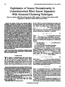
Fig. 1. Left: 3-D scatter plot of the data matrix ^ from Step 3.1 of Algorithm 1, in which one point corresponds to a column value of the matrix. Middle: Plot of all entries in the first row of the matrix. Right: Plot of some entries in the first row of the matrix and some bins (shown by red lines) (see Step 3.2.1) for detecting horizontal lines in Example 1.

Now we use Algorithm 1 to estimate the mixing matrix , based only on the observed mixture matrix . Noting that the indexes of the 1000 source columns with only one nonzero entry are not disjointed (corresponding to the disconnected time points), the DUET and the TIFROM algorithms thus cannot be used for estimating the mixing matrix in such case. Considering that the data set is artificial and that noise is absent, we do not need to carry out Steps 1 and 2. By carrying out Step 3, we obtain the set of estimated columns as in (11), shown at the bottom of the page. Comparing the columns of with those of , we can see that Algorithm 1 works well, although only 10% of the column vectors of are sparse (i.e., only one entry has a nonzero value). We tried the standard -means clustering method to estimate the columns of . However, we did not obtain any satisfactory results. The -means method does not work here, because there is a very small fraction of sparse source column vectors. The left subplot of Fig. 1 shows the three-dimensional (3-D) produced in scatter plot of all column values of the matrix Step 3.1 of Algorithm 1. The middle subplot of Fig. 1 shows the values of all entries in the first row of the matrix. Of course, cursory inspection of these two plots reveals that no cluster is visible. The right subplot of Fig. 1 shows the values of some entries in the first row of the matrix and some bins (see Step 3.2.1). Note that the right subplot shows the portion of the middle subto height . In our algorithm, we mainly plot from height use these bins to detect the horizontal lines mentioned above. As we indicated above, the heights of these horizontal lines represent the entries of the mixing matrix. The left subplot of Fig. 2 shows all entries of the matrix produced in Step 3.2.2 of Algorithm 1, in which we can see several line segments interspersed with other points. The heights of these line segments correspond to the entries of the first column of the mixing matrix up to a scale. Since we need a more precise estimate, we continue this procedure to further reduce the . matrix

X

~ Fig. 2. Left: Plot of all entries of the matrix ( ~

) from Step 3.2.2 of ~ ~

Algorithm 1. Right: Plot of all entries of the reduced matrix Step a2 of Algorithm 1 in Example 1.

X

from

The right subplot of Fig. 2 shows all entries of a matrix from Step a2 of Algorithm 1, in which we can see three “clear” line segments. The three line segments are formed with their heights correby three rows of the matrix sponding to the three entries of the first column of the mixing matrix up to a scale. The normalized mean column vector of is an estimated column of the mixing matrix the matrix (one of the columns of ). Finally, we present some information about the five free parameters in Algorithm 1. Because we carried out this simulation in the time domain and in the absence of noise, Steps 1, 2, and parameter are not needed. The other four parameters are , and .

III. LINEAR PROGRAMMING ALGORITHM FOR ESTIMATING SOURCE MATRIX AND RECOVERABILITY ANALYSIS After the mixing matrix is estimated, the next step is to recover the sources. This is carried out by using the linear programming algorithm in this paper. However, there is a recoverability problem; that is, rephrased as a question, Under what condition is the solution obtained by linear programming equal to the sources? This problem was preliminarily addressed and discussed in [12]. In this paper, we extend and improve the results in [12] from the viewpoint of probability and obtain several new results. In this section, we first extend the results of [7] and [5] by obtaining a sufficient and necessary condition for recoverability of a source column vector. Then, we establish and prove several probability inequalities that show the qualitative changing tendencies of probability of recoverability with regard to the sparsity of sources, the number of sources, and the number of sensors.

(11)


Given that the sources are sufficiently sparse in the time domain, the source matrix can be found by solving the following linear programming problem similarly as in [1], [7], [8]: (12) are entries of . where If the sources are not sufficiently sparse in the time domain, we can consider the following linear programming problem in the TF domain: (13) where are entries of . After is estimated, can be obtained by inverse wavelet packets transformation. In the previous section, we discussed estimating the mixing matrix, mainly in the TF domain. Hence, to obtain the coherence with the discussion of the previous section, it is better to discuss the recoverability based on the model (13). However, to simplify the notations, we base the discussions outlined in this and the next sections (on recoverability and the probability estimation of recoverability) only on the problem (12). Consequently, we find that the discussions in the two sections are also suitable for the model (13). Now we analyze the recoverability. Consider the optimization problem

where . (i.e., the number of nonzero entries of is ), . In the following, let denote a solution of . Note that can be of in (12). considered to be one column In [7], Donoho and Elad presented a sufficient condition, that is, less than 50% concentration implies equivalence between the -norm solution and -norm solution (the definition of -norm solution can be seen in [7] and [12]). In the following theorem, we extend the result presented in [5] and [7] into a sufficient and necessary condition. denote the index set of nonzero entries of , i.e., Let . denotes the set of all subsets of except the null set. Note that the cardinality of is . Theorem 1: 1) , if and only if, , when the following optimization problem (14) is solvable, its optimal value is less than

for for 2) Specifically, if independent, then

, and any two columns of .

(14) are

429

represents the number of In Theorem 1, -norm nonzero entries of . The proof of this theorem is presented in Appendix I. Theorem 1 is fundamental for the subsequent discussion. , there are a total Remark 2: For different subset optimization problems as (14), of which only some are solvable. The sufficient and necessary condition in Theorem 1 relates only to these solvable optimization problems. From Theorem 1, we can obtain the following corollary, which has appeared in [13] and [14]. Corollary 1: Given the mixing matrix , the recoverability of a source column vector by solving the problem does not depend on the magnitudes of its entries but only on the index set and signs of its nonzero entries. Now we assume that all entries of are drawn from a fixed probability distribution (e.g., uniform distribution valued in an interval); all nonzero entries of are also drawn from a fixed probability distribution (e.g., Laplacian distribution). The indexes of nonzero entries of are also taken randomly, and . In the following, we will consider the probability of recoverability, which is related , the number of sources , to the number of observations and the number of the nonzero entries of the source column . Let us define the conditional probability vector (15) We will analyze the conditional probability in three different cases: i) and are fixed; ii) and are fixed; iii) and are fixed. Using Theorem 1, we will prove three probability inequalities with regard to recoverability. Case i) and are fixed. We have the following theorem. Theorem 2: For fixed and , we have . The Proof of Theorem 2 is presented in Appendix II. The probability inequalities in Theorem 2 describes quantitatively the changing tendency of probability with respect to the number of zero entries of a source vector. That is, the higher sparsity of a source vector is, the higher probability of recoverability is. Case ii) and are fixed. Suppose that . Now we consider the following two optimization problems: (16) (17) and denote and the solutions of (16) and (17), respectively. and in (16) Theorem 3: Suppose that all entries of and (17), respectively, are drawn randomly from a distribution, are drawn randomly from a distriall nonzero entries of bution, and the indexes of their nonzero entries are also taken . Then, we have randomly, ; that is, . The proof is presented in Appendix III. The probability inequality given in Theorem 3 reflects the changing tendency of probability with respect to the number of sources. That is, the larger the number of sources is, the less the probability of recoverability is.

430


Case iii) and are fixed. Suppose that

optimization problem (14) is equivalent to the following optimization problem: . Consider the following

two optimization problems: (18) (19) and as the solutions of (18) and (19), and also denote respectively. in (18) in (19) Theorem 4: Suppose that all entries of are drawn randomly from a distribution, all nonzero entries of are drawn randomly from a distribution, and the indexes of its nonzero entries are also taken randomly. Then, we have ; that is, . The proof is similar to that of Theorem 3, which is presented in Appendix III. The probability inequality in Theorem 4 reflects the changing tendency of probability with respect to the number of sensors. That is, the larger the number of sensors is, the higher the probability of recoverability is. The qualitative tendencies of change in the probability of recoverability qualitatively shown in the inequalities above were first identified via simulations in [12]. However, the three inequalities of Theorems 2, 3, and 4 were neither stated explicitly nor proven in [12].

for

for

(20)

For , define , where . Denote the submatrix composed of all columns of with their column indexes being in , and the column vector composed of all entries of with denote their indexes being in . Then, (20) can be converted into the following optimization problem:

for for (21)

IV. PROBABILITY ESTIMATION In the previous section, we presented several probability inequalities showing the qualitative changing tendencies of the probability of recoverability. In this section, we assume that the mixing matrix is given or estimated. We will estimate analytically the probability that a source vector can be recovered by with a given or essolving a linear programming problem timated mixing matrix. Three cases are considered: 1) when the number of nonzero entries of the source vector is fixed; 2) when the number of nonzero entries of the source vector is unknown and when the probability is known that every entry of a source vector is equal to zero; 3) when all entries of a source vector are drawn from a Laplacian distribution. The probability estimate of recoverability can give us new insights into the performance and limitation of the linear programming algorithm when it is used to recover sources. For instance, if we know (or estimate) the probability distribution of source data, then we can estimate the probability of recoverability and decide whether the recovered sources are acceptable. Furthermore, if we know (or estimate) the number of sources, we can estimate how many sensors should be available in order for the sources to be recovered with high probability. First, we present several notations for the index set. Let , and denote the index set of nonzero entries of , as in the previous section. Obviously, there are index subsets of with cardinality . Denote these subsets as . The probability estimate is mainly based on the sufficient and necessary condition of Theorem 1. It is not difficult to find that

Furthermore, (21) can be converted into the following optimization problem:

for for (22) Noting that the sign function is known, thus (22) is a standard linear programming problem. Using the fact that an optimal solution of (22) satisfies , for , we can prove that the two optimization problems (14) and (22) are equivalent to each other. For a given or estimated mixing matrix, we consider three cases and estimate the probabilities of recoverability in the following. Case a) is the number of nonzero entries of a source column is fixed. vector We estimate the conditional probability , where . From Theorem 1, we have . It is well known that has at most nonzero entries; thus is not equal to when , that is, for .


Suppose that has nonzero entries; then, the index set of its nonzero entries is . Using , we define a sign in . column vector Note that if . It follows from Theorem 1 and Corollary 1 that the recoverability of a source vector is only related to the index set and sign of its nonzero entries, not to the amplitudes of its nonzero entries. Thus, the recoverability of is equivalent to that of . and a sign column vector in , For a given index set , the optimal value of (14) is if for any nonnull subset , i.e., the optimal value of (22) is greater than less than , then can be recovered by solving the linear program. ming problem Noting that there are sign column vectors in , suppose that there are sign column vectors that can be recovered. is the probability that a source vector , with its Then, , can be recovered by solving nonzero entry index set being . Furthermore, we have

Noting that say that

431

and are small, thus if . Hence, we have

is equal to

, we can (27)

where . are Remark 4: Because the entries of the source vector drawn from a Laplacian distribution, these entries are small but generally not equal to zero. Since we can see that has at most nonzero entries; thus, the equality does not hold can be very small. generally. However, the difference , we say that can be recovered. In this case, if In view that all entries of are drawn from a Laplacian distribution, it can be found that , denoted as . The probability that has entries greater than is , i.e., . Similar to (25), we have

(23) (28) where . Remark 3: When the mixing matrix is given or estimated, then the key number in (23) can be determined by checking whether the sufficient and necessary condition (14) is satisfied for all sign-column vectors. , supCase b) is as follows: For any source vector pose that the probabilities (24) We can find that the probability that has nonzero en. Next, we estimate the probability tries is . Noting that , we have

Obviously, it is reasonable to set a small positive first, and then find the bound according to . However, it is very difficult to estimate precisely the bound using . In the second simulation (Example 2) of Section V, is set to 0.06, and is set to . With these values for the two parameters, the estimated probability in (28) reflects well the true probability of recoverability for Laplacian source vectors. In this section, based on the necessary and sufficient condition in Theorem 1, several probability estimation formulas have been derived for different cases. These probability estimates reflect the true probability that the 1-norm solution is equal to the source vector. V. SIMULATION EXAMPLES

(25) are Case c) is as follows: All entries of the source vector drawn from a Laplacian distribution with probability density . This generally means that has function nonzero entries. Using , define a column vector : if , if , where is a small positive constant. with replaced by Consider the optimization problem , and denote its -norm solution . The -norm solution of corresponding to is still denoted as . It follows from the robustness analysis of the -norm solution in [12] that, for a given small positive constant , if is , i.e., . Thus, if sufficiently small, then an entry of satisfies , it can be considered to be a zero entry. Moreover (26)

The simulation results presented in this section are divided into three categories. Example 2 is concerned with the probability estimation of recoverability of the first two cases presented in the previous section [Cases a) and b)]. Example 3 is concerned with the probability estimation of recoverability in Case c) presented in the previous section. From these simulations, we can see that the probability estimates obtained in this paper reflect well the true probabilities with regard to recoverability. In Example 4, an underdetermined BSS problem is solved using the approach developed in this paper; we also compare Algorithm 1 with the standard -means clustering algorithm. is given in advance. Example 2: Suppose that This example contains two parts in which the recoverability probability estimates (23) and (25) are considered in simulation, respectively. I) For every index set , we first find the number of sign column vectors that satisfy the conditions of Theorem 1 and then we using (23). Noting calculate the probabilities

432


Fig. 3. Curves for estimated probabilities and true probabilities in Example 2. The left subplot is for Case a), while the right subplot is for Case b) of the consideration in Section IV.

that and , we thus obtain nine probabilities that are depicted by the “ ” and the solid curve in the first subplot of Fig. 3. , we take 3000 source Next, for every vectors, each of which has exactly nonzero entries. The nonzero entries are drawn from a uniform distribution , and their indexes are also taken ranvalued in domly. For each source vector, we solve the linear proand check whether the -norm gramming problem solution is equal to the source vector. Suppose that source vectors can be recovered; thus, we obtain the ratio that reflects the fraction of recovered source vectors among the 3000 source vectors. All are depicted by the “ ” and the dashed curve in the first subplot of Fig. 3. The two curves virtually overlap, which means that the probability calculated by (23) reflects the recoverability of a randomly taken source vector with nonzero entries. II) Now we consider the probability estimate (25). For , we calculate the probabilities in (25), noting that was obtained in the part I). Next, we define 3000 source vectors as follows: if if where

(29)

is drawn from a uniform distribution valued in . From (29), we can see that the probability is that each entry of a source vector is equal to zero. As in I), for each source vector, we solve the linear programand check whether the -norm solution is ming problem equal to the source vector. Suppose that source vectors can , be recovered; thus, we obtain the ratio which reflects the fraction of recovered source vectors among the 3000 source vectors. In the second subplot of Fig. 3, are depicted by “ ” and the solid curve, while are depicted by “ ” and the dashed curve. We see here also that the two curves fit very well, virtually overlapping. Thus, if we know the probability that each entry of a source vector is equal to zero, using (25), we can estimate the . probability that the source can be recovered by solving Conversely, if we set a lower bound of probability that a source

Fig. 4.

Curves for estimated probabilities and true probabilities in Example 3.

Fig. 5. Eight sources in Example 4.

vector is recovered, we can obtain the corresponding lower bound of the probability that each entry is equal to zero from (25). From this example, we can see that the probability estimates (23) and (25) reflect well the true probability that a source in Cases a) and b), vector can be recovered by solving respectively. is the same as that Example 3: The mixing matrix of Example 2. The aim of this example is to check by simulation whether the probability estimate (28) reflects the recoverability. First, we set the parameters and in Case c) of the previous section to 0.06 and 0.023, respectively. For 20 different Laplacian distributions with parameters , we calculate the probabilities using (28), noting that are from the Example 1. Next, for every 3000 source vectors are drawn from a Laplacian distribution with parameter . For is each source vector , the linear programming problem solved. If the -norm solution satisfies , then we say that can be recovered. Suppose that there are source . vectors recovered, we obtain the ratio (solid curve with “ ”) Fig. 4 shows the curves of and (dashed curve with “ ”). Here, the two curves also , the overlap remarkably well. In this example, for is reasonable. From Fig. 4, we can see that selected as the parameter in the Laplacian probability density function increases, the source vector becomes more and more sparse, and thus the probability of recoverability increases. Example 4: Consider the linear mixing model (1), where source matrix is composed of eight speech signals shown in Fig. 5. A 5 8 dimensional mixing matrix is selected randomly, and every column of is normalized to unit length. Only five mixtures are observable, shown in the subplots of the first row in Fig. 6.


Fig. 6. Blind source separation results of Example 4. First row: Five observable mixtures. Second and third rows: Eight recovered sources.

In this example, we first use Algorithm 1 to estimate the mixing matrix and do the comparison of our algorithm with a standard -means algorithm. Next, we estimate the sources using the linear programming algorithm. By Algorithm 1 (where the seven-level Daubechies wavelet packets transformation is used), an estimated 5 21 dimensional mixing matrix is obtained, denoted as . For each of , we choose one column of the 21 column column (if there is a column of the 21 vectors that is the closest to column vectors whose opposite vector is the closest to , we use its opposite vector). Thus, we obtain a submatrix denoted as . From the difference in (30), shown at the bottom of the is very close to the original mixing page, we can find that matrix . For comparison, we use the -means clustering algorithm to estimate the mixing matrix . The wavelet packets transformation coefficient set obtained in Step 2 of Algorithm 1 is also used. After normalizing all column vectors to the unit norm, and setting the number of clusters to be 21, we use the -means method to estimate the mixing matrix. From the resulting 21-cluster center vectors, we find a submatrix , as above, which is close to the mixing matrix . The difference and is presented as follows, (Please see the between equation at the bottom of the page.) From (31), shown at the bottom of the page, we can see that the estimates of the

433

first, the fourth, and the fifth column vectors of are not good (shown in bold faces). In our experience, those poorly estimated columns reflect poor recovery of corresponding sources. From (30) and (31), we can see that the estimate obtained using our method is better than that obtained using the standard -means algorithm. in addition, if we use a smaller cluster number when performing the -means algorithm, the difference becomes greater. Next, we estimate the source matrix . Using the estimated 5 21 dimensional mixing matrix, we solve the linear programming problem (13) and obtain the TF matrix . Applying the inverse wavelet packets transformation to every row of , we obtain 21 outputs in the time domain. Among these outputs, there are 13 outputs with obviously small amplitudes, which correspond to the columns of , far from the columns of . By removing the 13 columns of corresponding to these small outputs, a 5 8 dimensional (reduced) submatrix, still denoted as , remains. Using the matrix , we solve the linear programming problem (13) and apply the inverse wavelet packet transformation to estimate the source matrix again. The eight outputs are our recovered sources. The subplots in the second and third rows of Fig. 6 show the eight estimated signals, from which we can see that all the sources have been recovered successfully. Now, we consider a noisy model (2) with 27-dB SNR additive Gaussian noise. Using the proposed Algorithm 1, an estimated . 5 13 dimensional mixing matrix is obtained, denoted as From , we find a submatrix, as above, denoted as . From the difference in (32), shown at the bottom of the next page, is very close to the true mixing matrix we can find that , except that one column is poorly estimated (shown in bold faces). For comparison, we also use the -means clustering algorithm to estimate the mixing matrix , where the number of clusters is set to 13. From the obtained 13 cluster-center vectors, , which is close to we find a submatrix, as above, denoted as the mixing matrix . The difference between and is presented as (33), shown at the bottom of the next page, from which

(30)

(31)

434


we can see four columns are poorly estimated. From (32) and (33), we see that a better result is obtained using Algorithm 1. From [12], we can see that the linear programming algorithm for estimating the source matrix is robust to noise to some above, we can solve degree. Using the estimated matrix the linear programming problem (13) and estimate the source matrix as in the noiseless case above. Although we have obtained satisfying estimation of sources under 27-dB SNR additive Gaussian noise in our simulation, we omit the result here due to the limit of pages. Finally, we try using the TIFROM method to estimate the mixing matrix in the above noisy case. We find that we cannot obtain any satisfactory estimates of these columns of the mixing matrix. We first list the settings of the simulation example in [17]: three sources, including a stereo song and two voices from guitars (which are very sparse in the frequency domain), 60-dB SNR. Comparing these settings and those in our examples, we may conclude that relatively higher noise, larger source number, and wide-band sources lead to the violation of the sparsity condition of the TIFROM method. In addition, the variance operation used in the TIFROM method is not sufficient to detect the TF points precisely where only one source occurs. Thus, the TIFROM method does not work here. VI. CONCLUDING REMARKS In this paper, blind source separation was discussed using a two-stage sparse-representation approach. As in [8], the first stage estimates the mixing matrix, and the second stage estimates the source matrix. In general, estimating the mixing matrix and source matrix is carried out in the TF domain, since these signals are sparser than those in the time domain alone. We presented first an algorithm for estimating the mixing matrix, which can be seen as an extension of the DUET and the TIROFM algorithms but requires less stringent condition them. We then confirmed the validity of the algorithm by performing several simulations and by comparing these results with those obtained using a standard clustering algorithm, i.e., the -means clustering method. The sparseness condition can be considerably relaxed when using our Algorithm 1.

After the mixing matrix was estimated, we were also able to recover the source matrix using a standard linear programming algorithm. By extending the result in [5] and [7], we obtained a necessary and sufficient condition under which a source column vector can be recovered by solving a linear programming problem. Based on the established condition, several probability inequalities with regard to recoverability were established and proved easily. From these inequalities, we confirmed theoretically several intuitively obvious properties. That is, if the sparseness of sources increases, or the number of observations increases (the number of sources is fixed), then the probability of recoverability increases. If the number of sources increases (the number of sensors and the number of nonzero entries of the source vector are fixed), then the probability of recoverability will decrease. Furthermore, for a given or estimated mixing matrix, several theoretical probability estimates of recoverability were obtained in several different cases, e.g., the case in which the source entries were drawn from a Laplacian distribution. Simulation results showed that our theoretical probability estimates fit the true values very well. Finally, a blind speech source separation example was presented to illustrate the proposed approach. We would like to point out that, when using the two-step approach for blind source separation, it is not necessary to know (or estimate precisely) the number of sources in advance (see [12]). There still exists two challenging open problems: 1) if the source column vector is given or known, all entries of the mixing are drawn from a probability distribution; then how matrix does one estimate theoretically the probability of recoverability ; and 2) more generally, how does one estimate the in (15) when all entries of the unknown probability mixing matrix and source column vector are drawn from a probability distribution. APPENDIX I PROOF OF THEOREM 1 1. Necessity: Suppose that . optimal value of

; that is,

is the

(32)

(33)


For a subset , when (14) is solvable, there is at least a flexible solution. For any flexible solution of is a solution of the (14), it can be checked that constraint equation of , where with sufficiently small absolute value. We have

435

APPENDIX II PROOF OF THEOREM 2 From Theorem 1, it follows that . Now we prove the inequalities. Suppose that and that all nonzero entries of are taken randomly. Set . Consider the following two optimization problems: (39) (40)

(34) Thus

and denote and the two solutions of (39) and (40), respectively. From the definition of , we have . Denote the index set of nonzero entries of . Take a subset of such that the cardinality and define a column as follows: vector

(35)

if

if

(41)

Consider the optimization problem It follows from and (35) that . The necessity is proved. Sufficiency: Suppose that is a solution of the constraint equation in ; then, can be rewritten as (36) where Now we define an index set

.

. It can be checked easily that for the defined index set is a flexible solution of (14). From the condition of the theorem, we have . Furthermore

(42) where . The solution of (42) is denoted as . Since all nonzero entries of are from the nonzero entries of taken randomly, . Now suppose that . It follows from Theorem 1 that, , when the following optimization problem (43) is solvable, its optimal value is less than

for

for

(43)

, which is the index set of nonzero entries of , consider the following optimization problem:

for for (37) Note that the equality in the last step of (37) holds when (i.e., ). Thus, for any solution of the constraint equation in , we have (38) and the equality holds only when is equal to . Thus, . The sufficiency is proved. 2. The second and third conclusions in this theorem are obvious. Theorem 1 is proved.

(44)

such that it contains the indexes Define an index set of all nonzero entries of each of which has the same sign as a corresponding nonzero entry of . In view that is also a and that all nonzero entries of are taken from subset of , a flexible solution of (44) for the index set is also a flexible solution of (43) with the index set substituting for . Furthermore, from that , and that when , it is not difficult to find that . Hence, , where the second inequality is from the assumption of . From Theorem 1, we have . We can conclude that the equality implies . Thus, , i.e., for . Theorem 2 is proved.

436


APPENDIX III PROOF OF THEOREM 3 From , choose an index set that contains all indexes of nonzero entries of . Selecting the columns of with indexes , we obtain a dimensional matrix denoted as . Also selecting the entries with indexes , we obtain an dimensional of column vector denoted as . Consider the following optimization problem: (45) , and the solution of (45) is denoted as . where In view that is a -dimensional submatrix of , which is taken randomly from a distribution, and that all nonzero are the same as those of , also taken randomly, entries of . we have Now suppose that , and denote the index set of all nonzero entries of . It follows from Theorem 1 that, , when the following optimization problem (46) is solvable, its the optimal value is less than

for For the index problem:

for

(46)

above, consider the following optimization

for

for

(47)

When (47) is solvable, it is not difficult to find that a flexible solution of (47) can become a flexible solution of (46) by adding zero entries with corresponding indices. Thus, the optimal value of (46) is greater than or equal to that of (47), , given the asand the optimal value of (47) is less than . From Theorem 1, we have . In sumption of conclusion, the equality implies that . Thus, . Theorem 3 is proved.

REFERENCES [1] S. Chen, D. L. Donoho, and M. A. Saunders, “Atomic decomposition by basis pursuit,” SIAM J. Sci. Comput., vol. 20, no. 1, pp. 33–61, 1998. [2] B. A. Olshausen, P. Sallee, and M. S. Lewicki, “Learning sparse image codes using a wavelet pyramid architecture,” Advances in Neural Information Processing Systems 13, pp. 887–893, 2001. [3] M. S. Lewicki and T. J. Sejnowski, “Learning overcomplete representations,” Neural Comput., vol. 12, no. 2, pp. 337–365, 2000. [4] K. K. Delgado, J. F. Murray, B. D. Rao, K. Engan, T. W. Lee, and T. J. Sejnowski, “Dictionary learning algorithms for sparse representation,” Neural Comput., vol. 15, pp. 349–396, 2003.

[5] R. Gribonval and M. Nielsen, “Sparse representations in unions of bases,” IEEE Trans. Inform. Theory, vol. 49, no. 12, pp. 3320–3325, Dec. 2003. [6] J. A. Tropp, A. C. Gilbert, S. Muthukrishnan, and M. J. Strauss, “Improved sparse approximation over quasi-incoherent dictionaries,” presented at the 2003 IEEE Int. Conf. Image Processing, Barcelona, Spain, Sep. 2003. [7] D. L. Donoho and M. Elad, “Maximal sparsity representation via l minimization,” in Proc. National Academy Science, vol. 100, 2003, pp. 2197–2202. [8] P. Bofill and M. Zibulevsky, “Underdetermined blind source separation using sparse representations,” Signal Process., vol. 81, no. 11, pp. 2353–2362, 2001. [9] M. Zibulevsky and B. A. Pearlmutter, “Blind Source Separation by Sparse Decomposition,” Neural Comput., vol. 13, no. 4, pp. 863–882, 2001. [10] T. W. Lee, M. S. Lewicki, M. Girolami, and T. J. Sejnowski, “Blind source separation of more sources than mixtures using overcomplete representations,” IEEE Signal Process. Lett., vol. 6, no. 4, pp. 87–90, Apr. 1999. [11] M. Girolami, “A variational method for learning sparse and overcomplete representations,” Neural Comput., vol. 13, no. 11, pp. 2517–1532, 2001. [12] Y. Q. Li, A. Cichocki, and S. Amari, “Analysis of sparse representation and blind source separation,” Neural Comput., vol. 16, pp. 1193–1234, 2004. [13] J. J. Fuchs, “On sparse representations in arbitrary redundant bases,” IEEE Trans. Inform. Theory, vol. 50, no. 6, pp. 1341–1344, Jun. 2004. [14] D. M. Malioutov, M. Cetin, and A. S. Willsky, “Optimal sparse representation in general overcomplete bases,” presented at the IEEE Int. Conf. Acoustics Speech, Signal Processing (ICASSP), May 17–21, 2004. [15] A. Jourjine, S. Rickard, and O. Yilmaz, “Blind separation of disjoint orthogonal signals: Demixing N sources from 2 mixtures,” in Proc. 2000 IEEE Int. Conf. Acoustics, Speech, Signal Processing (ICASSP),, vol. 5, Istanbul, Turkey, 2000, pp. 2985–2988. [16] O. Yilmaz and S. Rickard, “Blind separation of speech mixtures via time-frequency masking,” IEEE Trans. Signal Process., vol. 52, no. 7, pp. 1830–1847, Jul. 2004. [17] F. Abrard, Y. Deville, and P. White, “From blind source separation to blind source cancellation in the underdetermined case: A new approach based on time-frequency analysis,” in Proc. 3rd Int. Conf. Independent Component Analysis Signal Separation (ICA), San Diego, CA, 2001, pp. 734–739. [18] F. Abrard and Y. Deville, “Blind separation of dependent sources using the time-frequency ratio of mixtures approach,” presented at the 7th Int. Symp. Signal Processing Applications (ISSPA), Paris, France, Jul., 1–4 2003. , “A time- frequency blind signal separation method applicable to [19] underdetermined mixtures of dependent sources,” Signal Process., vol. 85, no. 7, pp. 1389–1403, Jul. 2005.

Yuanqing Li was born in Hunan Province, China, in 1966. He received the B.S. degree in applied mathematics from Wuhan University, Wuhan, China, in 1988, the M.S. degree in applied mathematics from South China Normal University, Guangzhou, China, in 1994, and the Ph.D. degree in control theory and applications from South China University of Technology, Guangzhou, China, in 1997. Since 1997, he has been with South China University of Technology, where he became a Full Professor in 2004. He spent a few years at the Laboratory for Advanced Brain Signal Processing, RIKEN Brain Science Institute, Saitama, Japan, as a Researcher. Presently, he is an Associate Lead Scientist in the Institute of Infocomm Research, Singapore. He is the author or coauthor of more than 50 scientific papers in journals and conference proceedings. His research interests include automatic control, blind signal processing, neural networks, brain–computer interface, neural coding, and neural decoding.


Shun-Ichi Amari (F’94) was born in Tokyo, Japan, on January 3, 1936. He received the Dr.Eng. degree in mathematical engineering from the Graduate School of the University of Tokyo, Tokyo, Japan, in 1963. He worked as an Associate Professor at Kyushu University and the University of Tokyo, and then as a Full Professor at the University of Tokyo, where he is now Professor-Emeritus. He currently serves as the Director of the RIKEN Brain Science Institute. He has been engaged in research in wide areas of mathematical engineering, such as topological network theory, differential geometry of continuum mechanics, pattern recognition, and information sciences. In particular, he has devoted himself to mathematical foundations of neural network theory, including statistical neurodynamics, dynamical theory of neural fields, associative memory, self-organization, and general learning theory. Another main subject of his research is information geometry initiated by himself, which applies modern differential geometry to statistical inference, information theory, control theory, stochastic reasoning, and neural networks, providing a new powerful method of information sciences and probability theory. Dr. Amari is President of Institute of Electronics, Information and Communication Engineers (IEICE) of Japan and past President of the International Neural Networks Society. He received the Emanuel A. Piore Award and the Neural Networks Pioneer Award from the IEEE, the Japan Academy Award, the C&C award, among many others.

Andrzej Cichocki (M’96) was born in Poland. He received the M.Sc. degree (with honors), the Ph.D. degree, and the Habilitate Doctorate (Dr.Sc.) degree, all in electrical engineering, from the Warsaw University of Technology, Warsaw, Poland, in 1972, 1975, and 1982, respectively. Since 1972, he has been with the Institute of Theory of Electrical Engineering and Electrical Measurements at the Warsaw University of Technology, where he became a Full Professor in 1991. He spent a few years as an Alexander Humboldt Research Fellow and a Guest Professor at University Erlangen-Nuernberg, Germany, working in the areas of very large scale integration of electronic circuits, artificial neural networks, and optimization. He conducted and realized several successful research projects. From 1996 to 1999, he was working as a Team Leader of the Laboratory for Artificial Brain Systems, at the Frontier Research Program RIKEN (Japan), in the Brain Information Processing Group, and since 1999 he has been head of the Laboratory for Advanced Brain Signal Processing in the RIKEN Brain Science Institute. He is the coauthor of three books: Adaptive Blind Signal and Image Processing (New York: Wiley, 2003) with Prof. S.-I. Amari), MOS Switched-Capacitor and Continuous-Time Integrated Circuits and Systems (New York: Springer, 1989), and Neural Networks for Optimization and Signal Processing (New York: Wiley and Teubner Verlag, 1993–1994), both with Prof. R. Unbehauen). Two of his books have been translated to Chinese and other languages. He is also coauthor of more than one 150 papers. His current research interests include biomedical signal and image processing (especially blind signal/image processing), neural networks and their applications, learning theory and robust algorithms, generalization and extensions of independent and principal component analysis, optimization problems and nonlinear circuits, and systems theory and their applications. Dr. Cichocki is a member of several international Scientific Committees and has been the Associate Editor of the IEEE TRANSACTIONS ON NEURAL NETWORKS since January 1998.

437

Daniel W. C. Ho (SM’03) received the B.Sc., M.Sc., and Ph.D. degrees in mathematics (first-class) from the University of Salford, U.K., in 1980, 1982, and 1986, respectively. From 1985 to 1988, he was a Research Fellow in the Industrial Control Unit, University of Strathclyde, Glasgow, U.K. In 1989, he joined the Department of Mathematics, City University of Hong Kong, where he is currently an Associate Professor. His research interests include H-infinity control theory, robust pole assignment problems, adaptive neural wavelet identification, and nonlinear control theory. Dr. Ho is now serving as an Associate Editor for the Asian Journal of Control.

Shengli Xie (M’01–SM’02) was born in Hubei Province, China, in 1958. He received the M.S. degree in mathematics from Central China Normal University, Wuhan, China, in 1992 and the Ph.D. degree in control theory and applications from South China University of Technology, Guangzhou, China, in 1997. He is presently a Full Professor with the South China University of Technology and a vice head of the Institute of Automation and Radio Engineering. His research interests include automatic control and blind signal processing. He is the author or coauthor of two books and more than 70 scientific papers in journals and conference proceedings.