Optimal Activation and Transmission Control in Delay Tolerant Networks

inria-00408520, version 1 - 30 Jul 2009

Optimal Activation and Transmission Control in Delay Tolerant Networks Eitan Altman and Amar P. Azad

Tamer Bas¸ar

Francesco De Pellegrini

INRIA, 2004 Route des Lucioles 06902 Sophia-Antipolis Cedex, France {altman, azad}@sophia.inria.fr

Univ. Illinois, 1308 W. Main Urbana, IL 61801-2307, USA [email protected]

CREATE-NET, via Alla Cascata 56 c 38100 Trento, Italy [email protected]

Abstract—Much research has been devoted to maximizing the life time of mobile ad-hoc networks. Life time has often been defined as the time elapsed until the first node is out of battery power. In the context of static networks, this could lead to disconnectivity. In contrast, Delay Tolerant Networks (DTNs) leverage the mobility of relay nodes to compensate for lack of permanent connectivity and thus enable communication even after some nodes have depleted their stored energy. One can thus consider the life times of nodes as some additional parameters that can be controlled to optimize the performances of a DTN. In this paper, we consider two ways in which the energy state of a mobile can be controlled. Since both listening and transmission require energy, and since each of these has a different type of effect on the network performance, we study both the activation problem, which determines when a mobile will turn on in order to receive packets, and the transmission control problem, which can be done using transmission scheduling. The optimal solutions are shown to be of the threshold type. The paper introduces new methods to derive the threshold structure of optimal policies as previously used methods are not useful in this context due to the multidimensional nature of the problem. The findings are validated through extensive simulations. Index Terms—Optimal control, fluid models, delay tolerant networks, threshold policies

I. I NTRODUCTION During the last few years, there has been a growing interest in delay tolerant mobile ad-hoc networks [1], [2]. In such networks, no continuous connectivity guarantee can be assumed [3], [4]. Nevertheless, messages can still arrive at their destination thanks to the mobility of some subset of nodes that carry copies of the message. One central problem in DTNs is the routing of packets towards the intended destination, since mobile nodes rarely possess a priori information on the encounter pattern. This is also known as the zero knowledge scenario [5], [6]. One possible solution is to disseminate multiple copies of the message in the network, enhancing the probability that at least one of them will reach the destination node within a given time window [4]. The above scheme is referred to as epidemic-style forwarding [7], because, just as in the case of the spread of infectious diseases, each time a message-carrying node encounters an empty node, the carrier may infect this new node by passing on a copy of the message, and the destination receives the message when it meets an infected node. In this paper, we refer to a more efficient variant of the plain epidemic routing, namely the two-hop routing protocol. The source transmits copies of its message to all mobiles it encounters, but the latter relay the message only if they meet the destination [8].

In this framework, we study the problem of optimal control of routing, with the objective being maximization of the probability of delivery of a message to the destination by a given deadline, while satisfying specific energy constraints. In our model we account for two major sources of energy consumption, namely, message forwarding and beaconing: a finite energy cost accrues every time a message is transmitted or received, while there is an additional energy cost due to the periodic beaconing performed at relay nodes in order to signal their presence to the source node. A fundamental tradeoff which arises due to energy constraints is that the more copies are released, the smaller is the message delay. However, this requires a larger energy expenditure due to message forwarding. Moreover, when relays are battery operated, a further tradeoff emerges because one may activate relay nodes at different points in time in order to better schedule the activation nodes with full battery charge, e.g. through a wake-up timer. Related works have shown the benefit of optimal activation of nodes in redundantly deployed sensor networks in [9]–[11]. Accordingly, we consider within the model we adopt the general case of bounded activation policies, which is the case when energy harvesting is performed from renewable sources, e.g. solar energy, thus imposing bounds on the fraction of devices that can be activated over time. Within the framework introduced above, one can control two specific variables to optimize the network performance. The first one is the power by which relay nodes operate their transceivers to either relay messages or beacon. The second one is the time instant at which relay nodes are activated. We compute the joint optimal control policies that maximize the probability of successful delivery of the message by some time T , given the energy constraints and a bound on the relay nodes activation rate. We work with fluid approximations of the system dynamics, and use tools from optimal control theory to obtain a closedform optimal policy, which is time varying (which therefore is dynamic) and is defined by two simple thresholds. Extensive simulations validate the model and the results. The structure of the paper is as follows. The next subsection presents related work, and lists the main contributions of this paper. The section that follows introduces the model and the optimization problem. In Section II-A, we develop an alternate formulation of the optimization that solves for the optimal joint activation and energy control, with some reference cases solved in closed form. In Section V, we discuss an extension of

2

the model to the case of unbounded activation rates. Section VI provides a validation of the fluid model and a numerical investigation that illustrates the usefulness and power of our optimal control approach. Section VII concludes the paper.

inria-00408520, version 1 - 30 Jul 2009

A. Related works The control of forwarding schemes has been addressed in the DTNs literature before. In [12], the authors propose an epidemic forwarding protocol based on the susceptibleinfected-removed (SIR) model [13] and tune the parameters of the underlying SIR model. Another work [14] describes the relative performances of different self-limiting strategies. In [6] and its follow-up [5], the authors optimize network performance by designing message relays. Works in the same vein as ours here are [15]–[17]. In [15] the authors consider buffer constraints and derive buffer scheduling policies in order to minimize the delivery time. In an earlier paper [17] we have provided a general framework for the optimal control of a broad class of monotone relay strategies. The more recent paper [18] employs stochastic approximation to avoid the explicit estimation of network parameters. The performance of the two-hop forwarding protocol along with the effect of the timers have been evaluated in [19]; the framework proposed there allows performance optimization by choosing the average timer duration. Optimal activation of nodes in redundantly deployed sensor networks has been studied earlier in [9]–[11]. A thresholdbased activation policy was shown to perform 3/4 of that of the optimal policy for dynamic node activation in [9]. In [10], spatial temporal correlation has been exploited to improve usable lifetime in environmentally powered sensor networks. Scheduling/controlling the activity nodes to exploit energy harvesting features has been studied in [11]. Major contributions: As indicated earlier, a customary objective in DTNs is to maximize the fraction of delivered messages and to minimize the latency between source and destination. Compared with the existing literature, this paper makes two main original contributions. First, we include in our network model a general timedependent activation policy that triggers the active periods of relays, and we also account for the impact of beaconing over large periods of time. Second, we provide a formulation rooted in optimization, which entails joint optimization of the activation control and the transmission control in order to maximize the delivery probability within a given deadline. The solution relates explicitly the maximum allowed energy expenditure, the delivery probability within a given deadline, and the constraints on the activation of mobiles. II. S YSTEM MODEL For ease of reading, we collect all the main symbols used in the paper in Table I. We consider a network of N + 1 mobile nodes, where one of them, the source, has a message to send to a destination node. We adopt the two-hops routing relay policy, so that the source relays to mobiles which do not have the message but a relay transfers the message if and only if

Symbol N ξ µ T X(t) X(t) E(t) U (t) V (t) K(t) x z D(t) ` h∗

Meaning number of nodes (excluding the destination) inter-meeting intensity active nodes death rate timeout value fraction of nodes having the message at time t (excluding the destination) – controlled dynamics; uncontrolled dynamics (U(t)=1) energy expenditure by the whole network in [0, t ] energy control at time t, U (t) ∈ [u, 1], u ≥ 0 activation rate at time t upper bound of the activation rate: 0 ≤ V (t) ≤ K(t) maximum number of message copies due to energy constraint :=X(0) CDF of the message delay optimal activation threshold optimal energy control threshold TABLE I M AIN NOTATION USED THROUGHOUT THE PAPER

it meets the destination node. This relay strategy is monotone [17] because the number of copies of the message increases over time. The time between contacts of any two nodes is assumed to be exponentially distributed with parameter ξ. The validity of such a model has been discussed in [20], and its accuracy has been shown for a number of mobility models (Random Walker, Random Direction, Random Waypoint). We assume that the message that is transmitted is relevant for some time T . We do not assume any feedback that allows the source or other mobiles to know whether the message has made it successfully to the destination within the allotted time T . Each mobile sends periodically beacons to inform the source that they are in radio range. The source can transfer the message according to its forwarding policy. A relay node may already have a copy of the message: for such a node beaconing is not required, which may save considerable amount of energy. In what follows, we assume that relays keep beaconing untill they get a message copy from the source. However still some node can switch to inactive state to save energy. Accordingly, we define the state of a tagged node as falling into three categories: i. inactive: the tagged node does not take part in any communication; ii. activated: the tagged node does not have a message copy, it keeps beaconing until it receives a message copy; iii. infected: a node with a message is active but it does not send beacons. We assume that once a node becomes infected, it preserves energy for the last transmission of the message to the destination node if it meets destination before time T . Notice that the average life time of a mobile may be considerably shorter than the bound T . This limited life time is due to constraints on the total energy consumed: routing is particularly convenient since a mobile does not use much energy in transmission; however, the impact of beaconing is non-negligible. In this respect we assume that the probability that an activated mobile empties its battery at time (t, t + δ) is given by µδu if it uses power u(t) during that period. A. The Control There are two parameters that are controlled:

inria-00408520, version 1 - 30 Jul 2009

3

a. activation rate control: inactive mobiles do not contribute to communications in the DTN and do not use energy. By activating less/more mobiles per unit of time, one can use resources when they may be needed more. Another way to view this control as addition of new mobiles in the system as a result of energy harvesting. b. transmission control: the beaconing transmission power is controlled in order to mitigate the battery discharge of activated relays. Let {Tn } be the sequence of instants where an encounter takes place between two mobiles. Only at these times the e may change, where X e is a Markov chain process state X that represents the number of nodes that have the message. We introduce next the main fluid models used in the rest of the paper. Approximation of Markov chains through differential equations is a well known technique; see for example [21] for a survey. In the literature, the use of fluid approximations is a standard tool in modeling epidemic forwarding [13], [22], [23]. The approximation is known to be tight for large populations of nodes; more precisely the sample paths of the e are known to converge in probability to the Markov chain X solution of the limiting differential equation, which represents the expectation of the number of copies of the message [21], denoted by X(t) in the following. Fluid Approximations Let X(t) be the fraction of the mobile nodes that have at time t a copy of the message. Let Y (t) denote the fraction of active mobiles at time t which do not have a copy of the message. V (t) denotes the activation rate at time t and U (t) denotes the transmission control. X(t) grows at a rate given by the following pair of coupled differential equations: ˙ X(t) = U (t)Y (t)ξ (1) Y˙ (t) =

−U (t)Y (t)(ξ + µ) + V (t)

(2)

The term U (t)Y (t)ξ above represents the increase in the number of mobiles with copies of the message: it is due to encounters between the source with active mobiles without messages where each of these encounters has rate ξ. We take, without any loss of generality, Y (0) = 0. We also assume that U (t) ∈ [u, 1] for some u > 0, and the activation rate V is bounded as 0 ≤ V (t) ≤ K(t), 0 ≤ t ≤ T, where K(t) is a piecewise continuous function. Without RT loss of generality, we further assume that 0 V (t)dt = 1. Let the set of functions V (·) satisfying these two constraints (non-negativity and upper bounds, and unit area) be denoted by V. Delivery Delay Distribution The probability distribution of delay Td , denoted by D(t) := P (Td < t) is given by (see [24, Appendix A]), Z t ³ ´ D(t) = 1 − (1 − z) exp − N ξ X(s)ds , (3) s=0

Note that because of monotonicity, maximizing D(t) is equivRt alent to maximizing s=0 X(s)ds.

Energy Consumption In what follows, we will consider the case when the total energy consumed by the network is bounded. Let ² > 0 be the energy consumed by the network for transmission and reception of a single copy of the message. Thus, the total energy consumed by the network for transmission and reception of message copies during [0, T ] is ²(X(T ) − X(0)). Moreover, the beaconing power used at time t by active relays is proportional to U (t)Y (t)ξ so that the energy expenRT diture in [0, T ] due to beaconing is µ 0 U (s)Y (s)ds, i.e., µ ξ (X(T ) − X(0)). Hence, it follows that the total energy consumed in time T is E(T ) = (² + µξ )(X(T ) − X(0)). B. The Optimization Problem Our goal is to obtain joint optimal policies for the activation V (t) and the transmission control U (t), with U (t) ∈ [u, 1], and V (·) satisfying the additional upper-bound and integral constraints introduced earlier, that solve max

{V (·)∈V,U (·)}

D(T ),

s.t. X(T ) ≤ x, X(0) = z ,

(4)

where x and z (x > z) are specified. Recall that maximizing RT D(T ) is equivalent to maximizing 0 X(t)dt. III. O PTIMAL C ONTROL The solution to the problem will be shown to consist of policies involving two thresholds, one beyond which we stop activating mobile terminals, and the other beyond which we stop transmitting beacons. Various methodologies have been developed to establish the threshold structure of optimal transmission policies in DTNs: one based on the Pontryagin maximum principle [17], another based on some sample path comparisons [18], some on stochastic ordering, etc. These approaches, developed in the context of DTNs with one type of population, are not applicable to our problem since the model is no longer scalar. Accordingly, we develop a new approach that establishes the optimality of a threshold type policy for the activation control, following which we use Pontryagin’s maximum principle [25]. To obtain the optimal solution we first hold U (t) ∈ [u, 1] fixed, carry out optimization with respect to V (·), and then we substitute the optimal V (·), V ∗ (·), back into the objective function and carry out a further maximization with respect to U ·). For the first step, it is convenient to write the integral of X(·) explicitly as a V ·), which turns out to be linear : Z T Z T X(t)dt = ξ m(t)V (t)dt , (5) 0

0

where m(·) is some appropriate function, an expression for which is provided in the next subsection. A. Optimal Activation Control With U (t) ∈ [u, 1] fixed, we now first justify the equivalence (5), with an explicit expression for m(·), and then show that m(·) is non-increasing. This will allow us to conclude that the optimum choice for V (·) is of threshold form.

4

Lemma 3.1: Equivalence in (5) holds, with the expression for m(·) given in the proof below. Proof : To derive the equivalent form, we solve the coupled equations (1)-(2) in terms of V (·) and U (·), with zero initial conditions. Further doing appropriate substitutions and integration by parts, we obtain, m(t) = Z(T )Φ(0, t) − Z(t)Φ(0, t) −T W (t)Φ(0, t) + tW (t)Φ(0, t).

(6)

where substitutions usedµin (6) are: ¶ Z t Φ(t, T ) = exp −(ξ + µ) U (s)ds , T

inria-00408520, version 1 - 30 Jul 2009

dW

=

U (σ)Φ(σ, 0)dσ,

dZ = dtW (t).

We refer to [26] for detailed proof. ♦ Lemma 3.2: m(t) is non-increasing in t for all U (·) ≥ 0, and is monotonically decreasing for U (t) > 0. Moreover, the expression for m(·), as given in (6), can equivalently be written Z T as m(t) = (T − s)U (s)Φ(s, 0)dsΦ(0, t) (7) t

Proof : The expression for m(t) in (6) can first be simplified Rs using W (s) = 0 dσU (σ)Φ(σ, 0) and deriving Z(t) = Rt tW (t) − 0 sU (s)Φ(s, 0)ds. The expression for m(t) in (7) now follows from direct calculations. d Using the fact that Φ(t, 0)Φ(0, t) = 1, and dt Φ(0, t) = (ξ + µ)U (t)Φ(0, t) , we obtain dm(t) = −(T − t)U (t) − (ξ + µ)U (t)m(t) , dt which is non-positive for all t ∈ [0, T ] since m(t) is nonnegative, and is strictly negative whenever U (t) > 0. ♦ Let us define ½ ¾ Z t (8) ` := inf t ∈ (0, T ] : K(s)ds = 1 . 0

In view of the results of Lemma 3.1 and Lemma 3.2, we have the following. Theorem 3.1: The optimal policy V ∗ exists and is given by ½ K(t) if 0 ≤ t ≤ `, ∗ V (t) = (9) 0 otherwise .

at time t, nodes are activate with positive probability from t onwards. Formally, we will employ the following Rδ Corollary 3.1: Let 0 V (s)ds > 0 for any δ > 0. Then, Y (t) > 0, ∀t > 0

Also, X(t) is a non-decreasing function for all t > 0, and monotone increasing function when U (t) is strictly positive. Remark 3.1: (Turnpike property) We note from Theorem 3.1 that for all T large enough (in fact for all T that satisfy RT K(s)ds ≥ 1), the optimal threshold ` is the same. 0 B. Optimal Transmission Control In the previous subsection we characterized the optimal activation policy. We now proceed to derive the optimal transmission policy. From Corollary 3.1, X(t) is a monotonic increasing function. Furthermore we notice that similarly to what was shown in [17], the controlled dynamics X with U (t) can be interpreted as a slower version of the uncontrolled dynamics of X, i.e., the dynamics obtained when U (t) = 1. In this subsection, we first derive the uncontrolled dynamics for a general activation policy. This will then enable us to derive the optimal control policy in closed form. 1) Uncontrolled Dynamics: Let X(t) denote the uncontrolled dynamics of the system: it is the fraction of infected mobiles when U (t) = 1 for 0 ≤ t ≤ T . Proposition 3.1: For a given activation policy V , the fraction of infected nodes under U (t) = 1 and X(0) = z is Z t ξ X(t) = (11) (1 − e−(ξ+µ)(t−s) )V (s)ds + z ξ+µ 0 Proof : From (1) and (2) we have ξ ξ ˙ ˙ Y (t) = X(t) + V (t) ξ+µ ξ+µ ξ+µ ⇒ Y (t) = (f (t) − X(t)) (12) ξ Rt ξ where we introduced f (t) := ξ+µ V (s)ds + z , which de0 pends only on the activation control. The uncontrolled version X(t) is obtained by substituting (12) in (1) for U (t) = 1, ˙ + (ξ + µ)X = (ξ + µ)f . The solution is : which leads to: X Z −(ξ+µ)t

Proof : Any activation policy V can be viewed as a probability measure over [0, T ]; let us call Q∗ and Q two random variables having density V ∗ and V respectively, where V ∗ is defined in eq. (9), and where V is an arbitrary other policy. By construction, P [Q > t] ≥ P [Q∗ > t]. Since m is continuous, for t ∈ I = m([0, T ]) we can define t = min(m−1 (t)) so that P [m(Q∗ ) > t] = P [Q∗ ≤ t] ≥ P [Q ≤ t] = P [m(Q) > t] which concludes the proof since Em(Q∗ ) ≥ Em(Q). ♦ In the rest of the development, we will assume that V (s), seen as a measure, is non-degenerate, i.e., when it is applied

(10)

t

Z (ξ+µ)s

e

X(t) = e

0

s

V (r)drds + z.

ξ

(13)

0

Further, by integration by parts we obtain (11). ♦ Remark 3.2: For any given activation policy V : we substitute (12) into (1) to obtain a single differential equation, which is equivalent to the original system (1)-(2), i.e., X˙ = U (t)ξg(X, t)

(14)

where g(X, t) := (f (t) − X(t)) ξ+µ ξ . Remark 3.3: Considering (11), if we let W (r) = −(ξ+µ)r

e

ξ ξ+µ (1

−

)1{r≥0} , the uncontrolled trajectory appears as the

inria-00408520, version 1 - 30 Jul 2009

5

convolution X = W ∗ V , i.e., it can be seen as the linear transformation of the basic two hops dynamics via the kernel V imposed by the activation policy. In fact, since we can interpret V as a measure with total mass 1, in the singular case, i.e., when µ = 0 and V = δ(t), we obtain X(t) = (1 − e−ξt ) + z, i.e., the case of plain two hops routing, as expected. We observe also that in case U (t) = c, t ∈ [0, T ], u ≤ c ≤ 1 is a constant energy control policy, a simple time-rescaling argument offers Z t ξ X(t) = (1 − e−c(ξ+µ)(t−s) )V (s)ds + z = X(c t). ξ+µ 0 (15) In the following using the uncontrolled dynamics of the system, we can obtain the explicit form of the optimal transmission control using the maximum principle [27]. 2) Optimal Control: Definition 3.1: A policy U restricted to take values in [u, 1] is called a threshold policy with parameter h if U (t) = 1 for t ≤ h a.e. and U (t) = u for t > h a.e.. Theorem 3.2: Consider the problem of maximizing D(T ) with respect to U (·) subject to the constraint X(T ) ≤ z + x, under the activation control V . i. If X(T ) ≤ x + z, then the optimal policy is U (t) = 1. ii. If X(uT ) > x + z, then there is no feasible solution. iii. If X(T ) > x+z > X(uT ), then there exists a threshold policy. An optimal policy is necessarily a threshold one in the form ½ 1 if t ≤ h∗ U ∗ (t) = (16) u if t > h∗ Proof : Parts (i) and (ii) follow immediately from the fact that X is monotonically non-decreasing. We thus proceed with part (iii), working under the assumption X(T ) > x > X(uT ). Fix any activation policy V ; then from the Remark 3.2 we need Z T to solve ˙ max X(t)dt, s.t.X(t) = U (t) ξ g(X(t), t) U (·)∈[u,1]

0

We use the maximum principle to solve this problem. Introduce the Hamiltonian H(X, p, U ) = X(t) + (ξ + µ)U (t)p(t) (f (t) − X(t)) . where p(·) is the co-state variable. Since H is linear in U , the optimal control takes the extreme values u and 1 depending on whether H is positive or negative (it will be clear from the arguments below that the case H = 0 occurs on a set of Lebesgue measure zero). From (12), we know that f (t) − X(t) > 0 for all t. Hence the sign of H depends solely on that of p. Thus we arrive at the simple optimality condition: ½ 1, if p > 0 (17) U (t) = u, if p < 0 The co-state variable is generated by p(t) ˙ = =

dH = −[1 − (ξ + µ)U (t)p(t)] dX −1 + (ξ + µ)U (t)p(t)

−

(18)

Notice that we already know (based on linearity) that there must be at least one switch; in fact, if there is a switch, the only viable control would be either U (t) = u or U (t) = 1 for all t ∈ [0, T ], which is not possible because cases (i) and (ii) are excluded by assumption. We now prove that the optimal policy is of the threshold type by showing that there can be only one switch. There are three cases to consider based on the sign of p(0) in (18). Let us first consider the case p(0) < 0: from (18) then U (0) = u and further from this we can say that p(0) ˙ < 0. This means that p(0+ ) < p(0) < 0. Hence p(t) will never change sign, which contradicts the switching condition. Let us next consider the case p(0) > 0 and −1 + p(t) U (t)(ξ + µ) > 0. This implies U (0) = 1 and p(0) ˙ > 0, + i.e., p(0 ) > p(0) > 0. Hence the sign of p(t) always remains positive and optimal control remains at U = 1. This again contradicts our assumptions. Hence the only remaining possibility is that p(0) > 0 but −1 + p(t) U (t)(ξ + µ) < 0. This implies U (0) = 1 but p(0) ˙ < 0, i.e., p(0+ ) < p(0). Notice that the sign of p(t) ˙ remains negative as long as p(t) is decreasing until time h when value p(h) = 0 is attained. Furthermore, p(h+ ) < 0 and p(h ˙ + ) < 0, and the same reasoning of the previous case applies. We see that the optimal control starts at U (0) = 1 but switches to U (h) = u and never returns back. This satisfies the switching condition and guarantees that optimal control has exactly one switch. The optimal control is then given by ½ u, if t > h∗ U (t) = (19) 1, if t ≤ h∗ where h∗ can be computed using the procedure above.

♦

IV. J OINT O PTIMAL C ONTROL The analyses above have clearly led to the complete solution of the optimization problem (4), which is captured below. Theorem 4.1: For the optimization problem (4), the solution is given by the optimal activation control V ∗ (t) applied jointly with the corresponding threshold policy (as optimal transmission control) given in Thm. 3.2. A. Activation and Transmission Thresholds We have seen that the optimal policies are characterized by two scalar quantities, ` and h∗ , taking values in (0, T ). One interesting question now is whether one should wait for all the nodes to be activated before switching off the transmission control or not, i.e., whether it should be h∗ ≤ ` or h∗ > `. If h∗ ≤ `, it is then possible to activate a smaller number of relays with consequent energy savings; thus it is of interest to know the relative order of the thresholds h∗ and `. For ease of following the development below, let us introduce X as the optimal dynamics for t ≥ h∗ : from (1)-(2) and fixing the control U (t) = u for t ∈ [h∗ , T ], with initial condition X(0) = X(h), we have ˙ + u(ξ + µ)X(t) = u(ξ + µ)f X(t)

6

Hence, the optimal dynamics for t ≥ h∗ is of the form Z t −u(ξ+µ)(t−h) X(t) = e eu(ξ+µ)s (ξ + µ)uf (s + h)ds 0

+X(h)e

−(ξ+µ)(t−h)

, t > h.

Notice that X(T ) = X(T ) = x. Without loss of generality we assume z = 0 in the rest of the paper unless specified, for the sake of simplicity. Theorem 4.2: IfT > max{h∗ , `}, then the following relation holds for the bound x and the threshold h∗ :

inria-00408520, version 1 - 30 Jul 2009

h∗ > `, if x > X(`) + ∆X(`, T ), (20) h∗ ≤ `, otherwise , Z ` ξ where X(`) = (1 − e−(ξ+µ)(`−s) )V (s)ds, ξ+µ 0 ³ ξ ´¡ ¢ ∆X(`, T ) = − X(`) 1 − e−u(ξ+µ)(T −`) . ξ+µ X(`) denotes the uncontrolled growth of X in t = (0, `] and ∆X(`, T ) refers to the increment in X in (`, T ] under the controlled dynamics (with U = u ). Proof : A detailed proof can be found in [26]. ♦ Moreover, when both threshold times coincide, i.e. h∗ = `, the bound x can be expressed as ξ x = X(T ) = X(`) + (1 − e−u(ξ+µ)(T −`) ). ξ+µ B. Uniform Activation We consider as an example the case K(s) = K0 , where R` R` K(t)dt = 0 K0 dt = 1, which forces the activation of 0 nodes to be spread uniformly over time. We consider u = 0 for the sake of simplicity. As was done in subsection IV-A, we consider the fraction of infected node as follows under the assumption h∗ > ` as in (4.2). However, since we have assumed u = 0, X(h, T ) = 0. Hence in this case the above holds when x > X(`). Proposition 4.1: The optimal threshold for constant activation is given by ½ min(tˆ, T ), if x > X(`) (h∗ > `) ∗ h = (21) min(t˜, T ), if x ≤ X(`) (h∗ ≤ `) where tˆ =

1 ξ(e(ξ+µ)` − 1) log , ξ ξ+µ (ξ + µ)2 `(x − z − ξ+µ ) 2

t˜ =

L(−e−(x`(ξ+µ)

)ξ + x`(ξ + µ)2 + ξ . ξ(ξ + µ)

Here L(.) denotes the Lambert function,1 which is real-valued on the interval [− exp(−1), 0] and always below −1.

1 The

C. Impact of time horizon T In the earlier sections we showed that optimal transmission control policy U ∗ is a threshold policy for finite (fixed) time horizon and state constraint problem. We extend our earlier results when the time horizon T is extended further to and analyze asymptotically the impact on optimal policies. Optimal activation policy V ∗ derived in earlier section clearly indicates that early activation is optimal (satisfying the rate constraint K(t)). We also saw that V ∗ is the same for T above some value `. We next study the impact of T on U ∗ . This is summarized in the proposition below. Define T m := sup{t : X(t) ≤ x} and T m := sup{t : X(t) ≤ x}. Proposition 4.2: Consider maximization of D(T ) subject to the constraint X(T ) ≤ z + x, under the optimal activation control V ∗ and transmission control U (t) ∈ [u, 1]. i. For u > 0, there is no feasible policy for any T > T m . ii. For u = 0, the optimal transmission policy when T → ∞ is given by, ½ U (t) = 1 if t ≤ T m ∗ A = (22) U (t) = 0 if t > T m . Proof : (i) is direct. (ii) follows directly from the fact that the optimal activation policy V does not depend on T . ♦ V. E XTENSION TO U NBOUNDED ACTIVATION In some cases, the activation rate may not be bounded: this is the case of timer-based activation of batches of relays. Thus, in this section we extend our model to the case of unbounded activation, i.e., we assume that, for some τ > 0, Z t V (s)ds ≤ Ku (t) ≤ 1 t−τ

+ξ)/ξ

Proof : A detailed proof can be found in [26].

Notice from above that h∗ is approximately linear in `. Uniform activation is also of interest because of the following reason. In a scenario such as energy harvesting, it is expected to have cyclic kind of activation, e.g. more nodes are activated during the day exploiting solar energy than are at night. In Proposition 5.1 in the next section, we show that the threshold h∗ depends on E[V ]. This allows us to approximate the uniform activation with appropriate parameters which may require simpler calculation. In [26], we also consider the cases of i) Linear activation: K0 = 2/`2 , and ii) Exponential activation: K0 = α/(exp(α`) − 1).

♦

Lambert function, satisfies L(x) exp(L(x)) = x. As the equation y exp(y) = x has an infinite number of solutions y for each (non-zero) value of x, the function L(x) has an infinite number of branches.

where Ku (t) ≥ 0 is a piecewise continuous function. Again, the activation rate is subject to the normalization condition RT V (s)ds = 1; furthermore, we impose Ku (0) = 0 without 0 loss of generality. In this case, the optimal activation threshold is X X ` := τ · max{k ∈ N| Ku (kτ ) < 1, Ku ((k + 1)τ ) ≥ 1} The main difference from the results derived in Section III-A is related to the explicit form of the optimal activation control. Also, the related uncontrolled dynamics under the optimal

7

N=200, τ=20000, µ=0, Uniform Activation

a.I)

1 ` = 0, 5000, 10000, 15000 s

0

0.5

1

1.5

2

2.5

3

t [s]

4

x 10

a.II)

Simulation

0.2

0.6

0.2

0.2

0.1

0.05

` = 0, 5000, 10000, 15000 s 0

0.5

1

1.5

2

2.5

3

3.5

t [s]

0 0

4 4

x 10

` = 0, 10000, 15000 s

0.6 0.4

0.4

Theory

0.15

0

0.8

0.8

D(t)

0.05 0

N=200, τ=20000, µ=0, Uniform Activation

1

0.1

h∗ /τ

X

c)

N=200, τ=20000, µ=0, Uniform Activation

Theory

0.15

X

b)

Simulation

0.2

x=0.05 x=0.1 0.2

0.4

`/τ

0.6

0.8

1

0 0

Simulation Theory

1

2

t [s]

3

4 4

x 10

inria-00408520, version 1 - 30 Jul 2009

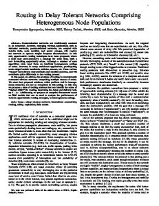
Fig. 1. a) Dynamics of the number of infected nodes under uniform activation, when ` = 0, 5000, 10000, 15000; upper part (a.I) depicts uncontrolled dynamics, the lower one (a.II) optimal dynamics for x = 0.1 b) CDF of the delay for optimal control: the thin solid lines represent the value attained by the uncontrolled dynamics. The case ` = 0 corresponds to plain Two-hops routing. c) Optimal Threshold under constant activation for two different values of x.

activation control can be expressed in a very simple form. The following theorem captures these. Theorem 5.1: Let the activation rate be bounded in the integral form. Let tk = kτ , k = 0, . . . , L−1 such that tL−1 < `, let tL = `Pand define ak = Ku (tk ), k = 0, . . . , L − 1, and aL = 1 − h ` Using the results for unbounded activation we can provide more insight in the role of V ∗ on the optimal success probability. As we will see in the following section, this result is very well confirmed by numerical results. In particular, consider an optimal (bounded) activation policy V ∗ and the related optimal transmission control. Let us consider u = 0 and z = 0 for the sake of simplicity. Assume h∗ > `, and let c = W 1{0≤u≤h∗ −`} W Z

Z

T

X(u)du = 0

0

h∗ −`

Z c (u)du W

h∗

Z ∗

V du = 0

0

h∗

c (u) W (23)

c (t) = 0 for t < 0, V ∗ has a finite where we used that W support, and the integral of the convolution is the product of the integrals. Now, let τ > 0 and consider the unbounded Rt activation obtained using as a bound Ku (t) = 0 V ∗ (u)du; we obtain ³ ξ ´ ˜ 1 E h∗ = log ξ ξ+µ ξ + µ ξ+µ − x PL −kτ ˜ where E = k=1 ak (τ )e . Taking the limit for τ → 0, we observe that Z ` ˜= lim E e−(ξ+µ)u V ∗ (u)du = GXV ∗ (ξ + µ) τ →0

0

where QV ∗ is a r.v. having density V ∗ , and GQV ∗ (ξ + µ) is the moment generating function calculated in ξ + µ. Thus we obtain the following result that holds for the bounded activation case: Proposition 5.1: Let optimal activation policy V ∗ be such that ` > h∗ ; then ´ ³ ξ G 1 QV ∗ (ξ + µ) h∗ = . log ξ ξ+µ ξ + µ ξ+µ −x Notice that, as a consequence of the above, using the standard moment series expansion for the moment generating function, we obtain GQV ∗ (ξ + µ) = 1 − (ξ + mu)EQV ∗ + 41 (ξ + µ)2 EQ2V ∗ + . . ., which leads to GQV ∗ (ξ + µ) = 1 − (ξ + µ)EQV ∗ + o(`2 (ξ + µ)2 ). Thus, under the assumptions of the proposition above, and when ` ¿ 1/(ξ + µ), we expect the tranmission threshold to be linear in EQV ∗ . Finally, according to (23), the system performance, i.e., D(T ) will be determined by the value EQV ∗ . VI. N UMERICAL VALIDATION Here we provide a numerical validation of the model. Our experiments are trace based: message delivery is simulated by a Matlab script receiving as input pre-recorded contact traces; in our simulations, we assume time is counted from the time when the source meets the first node, so that z = 1+Pa , where Pa is the probability that the first node met is active. Also, active nodes lifetime is an exponential r.v. with parameter µ. We considered a Random Waypoint (RWP) mobility model [28]. We registered contact traces using Omnet++ in a scenario where N nodes move on a squared playground of side 5 Km. The communication range is R = 15 m, the mobile speed is

8 N=200, T=20000, Uniform Activation, `=10000 1 x=0.1 x=0.05

0.9

D(T)

0.8 0.7 0.6 0.5 0.4 0.3 0

10

20

µ/ξ

30

40

50

inria-00408520, version 1 - 30 Jul 2009

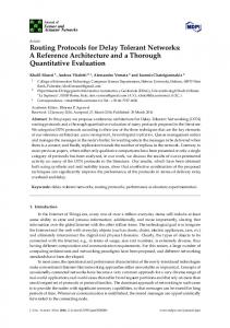
Fig. 2. Success probability for increasing values of µ/ξ, under uniform activation with ` = 10000 s and x + z = 0.05, 0.1, respectively.

v = 4.2 m/s and the system starts in steady-state conditions in order to avoid transient effects [29]. The time limit is set to T = 20000 s. Most graphs refer to the case N = 200. With the first set of measurements, we verified the fit of the activation model for the uncontrolled dynamics, i.e., when x + z = 1, and using a uniform activation policy. We assumed that µ = 0 and u = 0. We selected at random pairs of source and destination nodes and traced the dynamics of the infected nodes, see Fig. 1a.I); as see there and in the following figures the fit with the model is rather tight. The different curves seen in Fig. 1a.I) are obtained varying the constraint on the uniform activation policy; in particular the activation threshold ` = 5000, 10000, 15000. We included also the unbounded activation case when all relays can be activated at time t = 0; namely for ` = 0 and V = δ. As indicated there, in the case of constant activation the dynamics a change of concavity must occur (notice that X(∞) = 1). Indeed, see for example in [17], plain two hops routing has concave state dynamics. However, the change of concavity is an effect of ¨ = ξ(ξ + µ)Y − K0 the activation term, since (1)-(2) gives X which shows a sign switch when ` < T . Also, we depicted in Fig. 1b) the values of the optimal threshold for the transmission control in the case of uniform activation policy, at the increase of the activation threshold `. We considered two energy bounds x + z = 0.1 and x + z = 0.05. As we expected, a slower activation forces the optimal threshold to increase: as it appears in the figure, for the chosen activation constraint, the threshold increase is almost linear with `, showing congruence with (21). Notice that for the parameters chosen, we have ` < h∗ . The linear increase confirms the observation made in Prop. 5.1, since in both cases EQV ∗ = `/2 is linear in `. We repeated in Fig. 1a.II) the measurements of the dynamics of infected nodes and collected the CDF of the delay in the case of the optimal control in Fig. 1c). We can clearly observe the effect of the threshold policy on the dynamics of the infected nodes, since the increase of the number of infected stops at the threshold (u = 0). Conversely, we can observe that the delay CDF has a slightly lower curve compared to the uncontrolled case (reported with a thin solid line). So far, we did not consider the effect of µ on the success probability D(T ). Fig. 2 depicts the success probability for increasing values of µ. As expected, the higher the relative

magnitude of µ with respect to ξ, the lower the success probability. However, the effect of energy exhaustion due to beaconing takes over for larger values of µ and causes a much faster decay in case of looser constraints on energy (x + z = 0.1) than in the case of tighter ones (x + z = 0.05). Finally, we compared the effect of the activation bound on the success probability D(T ). In particular, we considered three alternative bounds: uniform, squared sine and exponential. In the case of a squared sine bound, we let K(t) = 2` sin2 ( π2 `t ). The comparison with the uniform activation shows that they result in a similar performance: as observed in Fig. 3a) the optimal transmission control and as a consequence the success probability (Fig. 3b)) as a function of ` is similar. This behavior is due to the fact that in both cases h∗ ≥ ` and the two activation measures have the same expected value. This confirms what was predicted in Prop. 5.1: in practice the system loses trace of the shape of the distribution as soon h∗ ≥ `. We also depicted the behavior in the case of a bound given by a truncated exponential where α = −70ξ: as seen in Fig. 3a) and Fig. 3b), the higher activation rate permits a larger success probability. This effect becomes dominant at larger values of ` and this results in the slower increase of the transmission threshold which saturates to a reference value; notice that this is a consequence of the exponential saturation of EQV ∗ with `, as observed already from Prop. 5.1. We repeated the measurements on the success probability D(T ) for increasing numbers of nodes, as reported in Fig. 3c). We can see the match of the uniform activation and the squared sine one. Also, we reported the behavior under truncated exponential activation in the case of |α| = 70ξ; the success probability in all these examples is seen to depend mostly on the expected value of V ∗ , as observed earlier. VII. C ONCLUSION AND F UTURE W ORK In this work, we have considered the joint optimization problem underlying activation of mobiles and transmission control in the context of delay tolerant mobile ad-hoc networks. Multi-dimensional ordinary differential equations are used to describe (the fluid limit of ) the associated system dynamics. Since the previously used approaches were not applicable to establish the structure of optimal activation policies, we devised a new method that is based on identifying the exact weight of the activation control at each time instant. We further validated our theoretical results through simulations for various activation schemes or constraints on activation. The control problems that we considered were formulated as maximization of the throughput subject to a constraint the energy. We note that we could have formulated the problem with soft constraints, instead of hard constraints, using a weighted sum of the throughput and the energy cost. We now argue that the optimal joint policy for this problem is of a double threshold type (i.e. both u and v have threshold structures). Indeed, the new problem can be viewed as the maximization of the Lagrangian that corresponds to the constrained problem. We can thus associate with the original problem a “relaxed” problem. For a fixed u, we have already seen that the cost

9

a)

N=200, τ =20000, x=0.1, µ=0.3ξ 1 0.9

b)

Uniform Squared sine Exponential α=−70 ξ

N=200, τ =20000, x=0.1, µ=0.3ξ

c)

1

0.9

0.9

0.8

0.7

0.7 0.6

0.6 0.5 0

D(τ)

D(τ )

h∗ /T

0.8 0.8

0.5 0.2

0.4

0.6

0.8

1

0.4 0

τ =20000, x=0.1, µ=0.3ξ 1

Uniform Squared sine Exponential α=70 ξ Exponential α=−70 ξ

0.7 0.6 0.5

Uniform Squared sine Exponential α=−70 ξ

0.2

0.4

0.4

`/T

0.6

`/T

0.8

1

0.3 0

50

100

N

150

200

Fig. 3. a) Optimal threshold as a function of ` b) Corresponding success probability D(T ) c) Success probability for increasing number of nodes. Different lines refer to the case of uniform (solid), squared sine and truncated exponential activation bounds

inria-00408520, version 1 - 30 Jul 2009

is linear in v(·). Therefore the Karush-Kuhn-Tucker (KKT) conditions are necessary and sufficient optimality conditions, which implies that a threshold-type v is also optimal for the unconstrained problem. To show that a double threshold policy is optimal for the relaxed problem we intend to show that there is a unique optimal policy for the constrained problem. R EFERENCES [1] S. Burleigh, L. Torgerson, K. Fall, V. Cerf, B. Durst, K. Scott, and H. Weiss, “Delay-tolerant networking: an approach to interplanetary Internet,” IEEE Comm. Magazine, vol. 41, pp. 128–136, June 2003. [2] L. Pelusi, A. Passarella, and M. Conti, “Opportunistic networking: data forwarding in disconnected mobile ad hoc networks,” IEEE Communications Magazine, vol. 44, no. 11, pp. 134–141, November 2006. [3] A. Chaintreau, P. Hui, J. Crowcroft, C. Diot, R. Gass, and J. Scott, “Impact of human mobility on opportunistic forwarding algorithms,” IEEE Transactions on Mobile Computing, vol. 6, pp. 606–620, 2007. [4] T. Spyropoulos, K. Psounis, and C. Raghavendra, “Efficient routing in intermittently connected mobile networks: the multi-copy case,” ACM/IEEE Transactions on Networking, vol. 16, pp. 77–90, Feb. 2008. [5] M. M. B. Tariq, M. Ammar, and E. Zegura, “Message ferry route design for sparse ad hoc networks with mobile nodes,” in Proc. of ACM MobiHoc, Florence, Italy, May 22–25, 2006, pp. 37–48. [6] W. Zhao, M. Ammar, and E. Zegura, “Controlling the mobility of multiple data transport ferries in a delay-tolerant network,” in Proc. of IEEE INFOCOM, Miami USA, March 13–17 2005. [7] A. Vahdat and D. Becker, “Epidemic routing for partially connected ad hoc networks,” Duke University, Tech. Rep. CS-2000-06, 2000. [8] R. Groenevelt, P. Nain, and G. Koole, “The message delay in mobile ad hoc networks,” Performance Evaluation, vol. 62, no. 1-4, pp. 210–228, October 2005. [9] A. Kar, K.; Krishnamurthy and N. Jaggi, “Dynamic node activation in networks of rechargeable sensors,” in Proc. of Infocom, March 13-27 2005. [10] A. Kansal, D. Potter, and M. B. Srivastava, “Performance aware tasking for environmentally powered sensor networks,” in SIGMETRICS ’04/Performance ’04: Proceedings of the joint international conference on Measurement and modeling of computer systems. New York, NY, USA: ACM, 2004, pp. 223–234. [11] T. Banerjee, S. Padhy, and A. A. Kherani, “Optimal dynamic activation policies in sensor networks,” in COMSWARE, 2007. [12] M. Musolesi and C. Mascolo, “Controlled Epidemic-style Dissemination Middleware for Mobile Ad Hoc Networks,” in Proc. of ACM Mobiquitous, July 2006. [13] X. Zhang, G. Neglia, J. Kurose, and D. Towsley, “Performance modeling of epidemic routing,” Elsevier Computer Networks, vol. 51, pp. 2867– 2891, July 2007. [14] A. E. Fawal, J.-Y. L. Boudec, and K. Salamatian, “Performance analysis of self limiting epidemic forwarding,” EPFL, Tech. Rep. LCA-REPORT2006-127, 2006. [15] A. Krifa, C. Barakat, and T. Spyropoulos, “Optimal buffer management policies for delay tolerant networks,” in Proc. of IEEE SECON, 2008.

[16] G. Neglia and X. Zhang, “Optimal delay-power tradeoff in sparse delay tolerant networks: a preliminary study,” in Proc. of ACM SIGCOMM CHANTS 2006, 2006, pp. 237–244. [17] E. Altman, T. Bas¸ar, and F. De Pellegrini, “Optimal monotone forwarding policies in delay tolerant mobile ad-hoc networks,” in Proc. of ACM/ICST Inter-Perf. Athens, Greece: ACM, October 24 2008. [18] E. Altman, G. Neglia, F. D. Pellegrini, and D. Miorandi, “Decentralized stochastic control of delay tolerant networks,” in Proc. of Infocom, April 19-25 2009. [19] A. A. Hanbali, P. Nain, and E. Altman, “Performance of ad hoc networks with two-hop relay routing and limited packet lifetime,” in Proc. of Valuetools. New York, NY, USA: ACM, 2006, p. 49. [20] R. Groenevelt and P. Nain, “Message delay in MANETs,” in Proc. of SIGMETRICS. Banff, Canada: ACM, June 6 2005, pp. 412–413, see also R. Groenevelt, Stochastic Models for Mobile Ad Hoc Networks. PhD thesis, University of Nice-Sophia Antipolis, April 2005. [21] R. Darling and J. Morris, “Differential equation approximations for markov chains,” Probability Surveys, vol. 5, pp. 37–79, July 2008. [22] R. Bakhshi, L. Cloth, W. Fokkink, and B. Haverkort, “Meanfield analysis for the evaluation of gossip protocols,” SIGMETRICS Performance Evaluation Review archive, vol. 36, pp. 31–39, December 2008. [23] A. Chaintreau, J.-Y. L. Boudec, and N. Ristanovic, “The age of gossip: Spatial mean-field regime,” in Proc. of ACM SIGMETRICS. ACM, June 2009. [24] T. Small and Z. J. Haas, “The shared wireless infostation model: a new ad hoc networking paradigm (or where there is a whale, there is a way),” in MobiHoc ’03: Proceedings of the 4th ACM international symposium on Mobile ad hoc networking & computing. New York, NY, USA: ACM, 2003, pp. 233–244. [25] G. Leitmann, Optimal Control. McGraw-Hill, 1996. [26] E. Altman, A. P. Azad, T. Basar, and F. De Pellegrini, “Optimal activation and transmission control in delay tolerant networks,” in available on Arxiv(arXiv:0907.4329). [27] D. P. Bertsekas, Dynamic Programming and Optimal Control. Athena Scientific, 1995. [28] T. Camp, J. Boleng, and V. Davies, “A survey of mobility models for ad hoc network research,” Wireless Communications & Mobile Computing (WCMC), vol. 2, no. 5, pp. 483–502, August 2002. [29] J.-Y. L. Boudec and M. Vojnovic, “Perfect simulation and stationarity of a class of mobility models,” in Proc. of INFOCOM. Miami, USA: IEEE, March 13–17 2005, pp. 183–194.