Vth in of a gate input is de ned as the voltage value .... ned traditional test vector selection strategies su er ..... 20 P. Banerjee, and J.A. Abraham, Characteriza-.
Optimal Voltage Testing for Physically-Based Faults Yuyun Liao
D.M.H. Walker
Dept. of Electrical Engineering Texas A & M University College Station, TX 77843
Dept. of Computer Science Texas A & M University College Station, TX 77843
Abstract
In this paper we investigate optimal voltage testing approaches for physically-based faults in CMOS circuits. We describe the general nature of the problem and then focus on two fault types: resistive bridges between gate outputs that cause pattern sensitive functional faults and opens in transmission gates that cause delay faults. In both cases, the traditional stuckat model is inadequate. The test vector to sensitize and propagate a resistive bridging fault is not unique. The traditional greedy test vector selection is optimistic, with some choices having poor real coverage. We realistically model the fault and fault coverage, and describe an optimal selection strategy. In a transmission gate with an open NMOS or PMOS device, the output voltage is degraded, increasing delay and reducing noise margin. We model this fault and show how lowvoltage testing can be used to detect it. Our goal in applying these techniques to all important fault types is to maximize the real coverage of voltage tests, thereby minimizing the number of relatively slow Iddq tests required to achieve high quality.
1 Introduction
The semiconductor marketplace drives manufacturers to develop production IC tests with higher fault coverage at lower cost. Of particular interest is better screening for functional and parametric faults at wafer test. This is especially important for known good die products. In recent years much research has been devoted to quiescent current (Iddq) testing as an addition to voltage testing of CMOS circuits to achieve higher test quality. The primary drawback of Iddq testing with standard ATE is that it is much slower than voltage testing. Newer current sensor designs [1] are much faster, but still much slower than voltage testing. There is also increasing concern that Iddq testing will be less e�ective in more advanced technologies [2]. In addition, Iddq testing is di�cult when the normal Iddq level is high, as is the case in high-
performance microprocessors, and many mixed signal devices. We can gain many of the bene ts of Iddq testing through more optimal voltage tests. The best test set combines both voltage and Iddq tests, but given the speed advantage of voltage testing and existing ATE investment, we should attempt to maximize the real fault coverage of voltage tests, using a small number of Iddq tests to target the remaining faults. The choices in voltage testing approaches can be categorized in the following fashion: 1. design and process information - layout, circuit, schematic, fault types, defect densities 2. fault modeling - stuck-at, simpli ed realistic, accurate realistic 3. test generation method - random, targeted, fault model used 4. test coverage analysis - fault model used 5. test conditions - test speed, supply voltage, temperature Standard approaches to voltage testing only use schematic information, assume a stuck-at fault model, assume all faults are equally likely, and use the datasheet supply voltage range. At the other end of the spectrum would be to use the design layout, fault densities, and accurate realistic fault models to compute realistic fault probabilities, and to target tests for them assuming a particular test speed, and selecting the optimal test voltages and temperature. More likely is a compromise to achieve good coverage at reasonable test generation cost. Our general approach is to rst develop an accurate realistic fault model. For example, most prior work on voltage test of bridging faults assumes that the bridge resistance can be neglected [3], [10]. But it
has been shown that bridge resistances are often large enough that they must be accounted for [16], so we include the bridge resistance in our model. Similarly, nearly all of the more than 100 papers published on opens [18] only deal with complete opens, not partial opens as can occur in a transmission gate. We then use the accurate model to develop improved test coverage metrics (potentially including process and layout information), evaluate existing test generation algorithms, and develop new test conditions and test generation algorithms if existing ones are not adequate. In the sections that follow we demonstrate these ideas on optimal voltage testing of resistive bridges and partially-open transmission gates. Section 2 of this paper investigates the characteristics of bridging faults in CMOS circuits, an accurate fault model, describes an accurate bridging fault coverage metric, and a test generation algorithm. Section 3 describes the characteristics of partially-open CMOS transmission gates, a low voltage test technique, voltage selection strategy, and test generation algorithm. Conclusions and future work are described in Section 4.
2 Optimal test vector generation for voltage testing of CMOS bridging faults
Shorts are the most common fault type in CMOS circuits [16]. Shorts can be divided into two subclasses: inter-gate and intra-gate shorts [15]. The inter-gate shorts are usually called external bridging faults. It has been demonstrated that a bridging fault causes a functional failure if the bridging resistance (Rsh ) is less than a certain value [15]. In order to sensitize a bridging fault, we try to set the nodes involved in bridging to opposite logic values [3]-[15]. The voltages at the bridged nodes depend on the activated pull-up network and pull-down network that are involved in bridging, transistor process parameters and bridging resistance. If the pull-up (pulldown) network has more than one sensitizable path from V dd (GND) to the bridged node, and more than one driven gate which can propagate the fault e�ect, the test vector is not unique. The test vector selection strategies previously published, which are called traditional test vector selection strategies in this paper, choose the rst test vector found. We will show that the fault coverage depends on the selected test vector, and the topologies of the gates connected to the bridged nodes. This implies that greedy algorithms may be optimistic. We then describe an optimal test selection strategy.
2.1 Driving circuit behavior
Consider the circuit shown in Fig. 1, which is the original circuit given in [15]. In order to detect a bridging fault, the nodes involved in bridging must be set to opposite logic values. Let us assume that we try to set node 1 to V dd, and node 2 to GND. To try to set node 1 to V dd, < A1; B1 > must be set to < 0; 0 > or < 0; 1 > (vector < 1; 0 > is equivalent to < 0; 1 > and neglected in this paper). Similarly, to try to set node 2 to GND, < A2; B2 > must be set to < 1; 1 > or < 0; 1 > (vector < 1; 0 > is equivalent to < 0; 1 > and also neglected in this paper). Hence, the possible values of test vector < A1; B1; A2; B2 > for bridging faults in Fig. 1 are < 0; 0; 1; 1 >, < 0; 0; 0; 1 >, < 0; 1; 1; 1 > and < 0; 1; 0; 1 >.
A1 B1 A2 B2
� A3 a f sV (1) �node1 R � �node2 b fs �V (0)B4 sh
.... ............. ............. ...
c
� f Q1 �
d
�Q2 f �
sh
sh
Figure 1: A circuit with bridging fault Next, we use HSPICE simulation to evaluate each of these test vectors in terms of maximum bridging resistance to be detected. All circuits used for bridging faults were constructed using OCTTOOLS standard library cells. All of the HSPICE simulations for the bridging faults are based on a 1.2� N-well CMOS technology. The maximum detectable bridging resistance by di�erent test vectors via outputs Q1 and Q2 are given in Table 1, where X indicates that no functional fault is exposed for the bridging resistance range from 0 to 1 . As can be seen, test vector < 1; 0; 1; 1 > and < 0; 0; 1; 0 > are the best candidates for testing via primary output Q1 and Q2 respectively in terms of the maximum detectable bridging resistance. In order to fully describe the characteristics of the driving gates involved in the bridging fault, it is necessary to derive the electrical equation to compute the intermediate voltages of the bridged nodes. For a CMOS gate, di�erent input combinations that produce the same logic value at the output of the gate may activate di�erent pull-up or pull-down paths with
Table 1: The maximum detectable bridging resistances for di�erent test vector test vector Rsh max Rsh max via Q1 via Q2 0010 X 1500
0011 100
300
1010 170
450
1011 1200
X di�erent equivalent resistance. When two nodes involved in bridging are set to opposite logic values, the resultant circuit can be simpli ed as a resistive divider between V dd and GND (illustrated in Fig. 2).
Vdd .....
.. .. .. .... ............. ... ...........
.... .............. .. ............... ... .
Rp
A3 Vtsh (1) ..... node1 ................. ............... R sh .... tnode2 Vsh (0)
Rn GND
B4
c
� f Q1 �
d
�Q2 f �
2.2 Driven gate behavior
Figure 2: Equivalent circuit of Fig. 1 The intermediate voltages (Vsh (1) and Vsh (0)), obviously, depend on the equivalent resistance of the pull-up network of gate a, the bridging resistance (Rsh ) and the equivalent resistance the pull-down network of gate b. Vsh (1) and Vsh (0) are expressed as, Vsh (1) = R + RRp + R V dd p sh n
First let us consider testing based on the evaluation of intermediate voltage Vsh (1). In order to achieve the highest fault coverage, Vsh (1) should be as low as possible. From equation (1), we know that the equivalent resistance Rp should be as large as possible and Rn should be as small as possible, that is, with the least possible number of activated pull-up paths and the most possible number of activated pull-down paths in the driving gates. Let us now consider testing based on the evaluation of intermediate voltage Vsh (0). In order to achieve the highest fault coverage, Vsh (0) should be as high as possible. From equation (2), we know that the equivalent resistance Rp should be as small as possible and Rn should be as large as possible, that is, with the most possible number of activated pull-up paths and the least possible number of activated pull-down paths in the driving gates.
(1)
Vsh (0) = R + RRn + R V dd (2) p sh n where Rp is the equivalent resistance of the pullup network of gate a, Rsh is the bridging resistance and Rn is the equivalent resistance of the pull-down network of gate b.
The logic interpretation of the intermediate voltages depends on the con gurations of the driven gates involved in bridging. To minimize ambiguity, a key term should be refreshed. The input logic threshold (Vth in ) of a gate input is de ned as the voltage value at which the input and output of the gate are equal (assuming all other inputs of that gate are held at non-controlling logic values)[3]. A small deviation of the input voltage above or below Vth in is su�cient to cause a large swing in the output. The logic interpretation of the intermediate voltages depends on the Vth in of the driven gates. Each input of each logic gate can have a di�erent input logic threshold. The implication of this behavior is that two driven gates tied to the same bridged node may interpret the same intermediate voltage as two di�erent logic values. This situation has been dubbed \The Byzantine General's problem" in [4]. The input logic thresholds for di�erent logic gates can be derived both theoretically and experimentally [3]. Fig. 3 is used to illustrated \The Byzantine General's problem". For testing based on the evaluation of intermediate voltage Vsh (1), the maximum detectable resistances via primary output Q0 and Q1 are 1.3K and 1.1K
respectively. Hence, to increase the detectable bridging resistance range, the driven gate with the highest input logic threshold should be selected as primary output for testing based on the evaluation of intermediate voltage Vsh (1). For testing based on the evaluation of intermediate voltage Vsh (0), the maximum detectable resistances via output Q2 and Q3 are 1.5K
and 1K respectively. In this case, the driven gate
� A3 a f sV (1) �node1 � �R b f snode2 �V B4
A1
sh
B1
.... ........... ........... ...
A2 B2
sh
sh(0)
Q0 HH f " "� c
f Q1 �
�Q2 d f � b� f Q3 �b
.
Figure 3: Another example circuit with a bridging fault Table 2: Bridging resistance distribution. Bridging resistance Number range single bridges Rsh � 0.5K 244 (69.3%) Rsh � 1K 337 (95.7%) Rsh � 5K 346 (98.3%) Rsh � 10K 349 (99.1%) Rsh � 20K 352 (100%) with the lowest input logic threshold should be sensitized.
2.3 fault coverage
The evaluation of fault coverage requires the knowledge of the bridging resistance distribution. Previous research showed that the metal bridging resistance mainly falls into the range from 0 to 1000 (illustrated in Table 2) [16]. We nd that a Geometric distribution has good agreement with the data in Table 2 ( the maximum error is less than 3%). The bridging resistance distribution function P (Rsh ) is: P (Rsh ) = 1 , (1 , p)Rsh (3) where p = 0.00258. The bridging fault coverage c(i) for bridging fault
Table 3: The bridging fault coverage for the bridging fault con guration in Fig. 1 under di�erent test vector test vector C via Q1 C via Q2 0010 0 97% 0011 22.7% 53% 1010 35.5% 69% 1011 96% 0 con guration i can be obtained in the following way: c(i) = 1 , (1 , p)Rsh max(i) (4) where Rsh max (i) is the maximum detectable bridging resistance for the bridging fault con guration i. The value of Rsh max (i) varies from node to node. The bridging fault coverage C for the whole circuit is:
X
N C = N1 c(i) i=1
(5)
where N is the total number of the bridging fault con gurations (assuming equally likely faults). The bridging fault coverage calculated by equation (4) for the bridging fault con guration in Fig. 1 under di�erent test vectors is given in Table 3. As can be seen, for testing via primary output Q1 in Fig. 1, the bridging fault coverage for test vector < 0; 0; 1; 0 > (a possible choice for traditional test vector selection strategies) is 0. In order to increase the fault coverage, the \Voting Model" was proposed [4]. The main drawback of this model is that the bridging resistance is assumed to be negligible. The \Parametric Model" was proposed for realistic resistance bridging fault [15]. This work demonstrated that the \Voting Model" developed for non resistive bridging faults does not adequately represent the behavior of realistic resistive bridging faults. This fault model can gure out which primary output will give better fault coverage, but it also uses the rst test vector found among several candidates. If test vector < 0; 0; 1; 1 > is picked up for testing, for example, the \Parametric Model" can gure out that testing via primary output Q2 will give better fault coverage. We call the test vector selection strategy based on the \Parametric Model" the re ned traditional test vector selection strategy. The fault coverage comparisons are given in Table 4, where the number in the bridging con guration name is the number of gate inputs. The driven gates of these bridging
Table 4: The bridging fault coverage comparison C for C for C for bridging random re ned optimal con guration strategy strategy strategy INV INV 69% 69% 69% NAN2 INV 35.7% 62.4% 87.3% NAN2 NAN2 35.7% 59% 96.4% NAN2 NOR2 46.7% 78.8% 96.5% NOR2 INV 35% 58% 93.4% NOR2 NOR2 46.1% 89.2% 98.8% con gurations are 2-input NAND gates. We assume that each of the possible test vectors has equal opportunity to be picked up. The bridging fault coverage data in Table 4 indicate that the traditional and re ned traditional test vector selection strategies su�er from optimism. Some of bridging faults that are not covered by optimal test algorithm may cause delay faults. Some of uncovered bridging faults don't cause faults at all. Although this paper focuses on the inter-gate shorts, the handling of intra-gate shorts can be achieved with straightforward modi cations that will not be mentioned here.
2.4 Testing generation for bridging faults
or computing time. But this step is not the dominant step in terms of time. Therefore, the time complexity of our proposed algorithm is the same as the time complexity of the traditional test vector generation algorithms.
3 Detection of \undetectable" open faults in CMOS transmission gate using low-voltage testing Opens in CMOS circuits are well-known for causing faults that cannot be modeled with the stuck-at model, such as degraded noise margin or delay faults. Researchers have investigated the problem of testing CMOS transmission gates (TG) for stuck-open faults [19]-[22]. But much of this work requires extra test hardware, and treats the transmission gate as a black box (i.e. they considered a CMOS transmission gate stuck-open as a whole). Probable open faults in a transmission gate are illustrated in Fig. 4. A signi cant fraction of these faults (d0, d1, d2 , d3 , d4, or d5 in Fig. 4) are not covered by [19]-[22]. d0 d1 d6
V in
Many algorithms are known, but they are all NPcomplete. All of these algorithms are based mainly on the following steps [17]: 1. 2. 3. 4.
Excite the fault. Find a sensitized path. Try to justify that path. If there is a con ict, go back to the last choice and try the other choice. 5. If this path cannot be justi ed, try another path. All of the traditional test algorithms for bridging faults can be used directly by our optimal test algorithm except the fault exciting step. This step is modi ed based on the optimal strategy mentioned in the previous subsections. The fault exciting step for the bridging faults tries to set the nodes involved in bridging to the opposite logic values. At this step, only the driving and driven gates of the bridged nodes are involved. The increased cost of this step, compared to the traditional algorithms, is the constrained searching
d2 d7
d4
V out
d5 Cl d3
C
Figure 4: CMOS transmission gate Open faults in NMOS or PMOS devices of CMOS transmission gate degrade the circuit timing performance without altering the logical function at normal power supply voltages. These opens are classi ed as \undetectable" and deleted from the fault list in traditional stuck-at models. These opens may be detectable via Iddq testing [23], but with the drawbacks cited previously. Instead we propose to use a low-voltage testing technique to detect these opens. Low-voltage testing may also be used to detect other types of faults [24], which will be described in a future work. We show below that transmission gates with these opens can be forced to exhibit stuck-at fault behavior at low power supply voltages. The advantage is that a traditional stuck-at test generator can be used
to target these faults, but test speed may have to be reduced.
3.1 Characteristics of CMOS transmission gate with open faults at di�erent power supply voltage
It is assumed that in a given CMOS transmission gate a single open fault occurs at a transistor source, drain or gate. In this paper we only consider opens at d0, d1, d2, d3, d4, or d5 in Fig. 4. Opens at d6 , d7 in Fig. 4 can be modeled by traditional stuck-open models. In this section we will examine CMOS logic circuit with a partially open transmission gate at di�erent power supply voltages. It will be shown that a CMOS circuit with open fault in n-channel or p-channel of transmission gate functions correctly at normal power supply voltage, and become faulty at a certain lower power supply voltage. Our testing technique is based on this voltage dependence characteristic. In order to get the HSPICE les for a given CMOS logic circuit with open fault in n-channel or p-channel in a transmission gate. We: 1. Create a MAGIC layout for a given CMOS logic circuit. 2. Modify the created MAGIC layout with a gap at drain, source, or gate line of CMOS transmission gate to mimic an open fault. 3. Extract the modi ed MAGIC layout to get .ext le. 4. Use ext2spice to extract the created .ext le to get the HSPICE le. Consider the CMOS logic circuit shown in Fig. 5 which is the transmission gate embedded latch given in [25]. The p-channel and n-channel transistors have sizes 12/2 and 6/2 respectively. The transistor sizes are chosen such that outputs have balanced rise and fall times. As an example, let us assume that there is an open fault at the drain of the p-channel transistor (d5 in Fig. 5). Fig. 6 shows the HSPICE simulation results for the latch at normal power supply voltage (Vdd =5V). Vout tg = 5 , Vtn when Vin = 5V , where Vtn is the n-transistor body a�ected threshold. Vtn is calculated as a function of Vsb (source-substrate voltage) in [25]. In the case we studied, Vsb equals to Vout tg . Vtn is expressed as in the following,
p
p
Vtn = Vtn0 + [ (2�b + Vout tg ) , 2�b ];
where Vtn0 is the n-transistor threshold voltage for Vsb = 0, is the constant that describe the substrate bias e�ect, and �b is the bulk potential. We notice that the output of the transmission gate is degraded. However,this degraded value is correctly interpreted by the driven gates, as shown by Vout . Vdd
Vdd
clk out d2 out_tg
in d5
Figure 5: Transistor schematic diagram of transmission gate embedded latch
Figure 6: Simulation for latch with open fault in pchannel of TG (Vdd =5V) Fig. 7 and Fig. 8 show HSPICE simulation results for latch with and without an open fault in the pchannel of the CMOS transmission gate for Vdd =2V respectively. We notice that the latch without the open fault still function correctly at Vdd =2V while the latch with an open fault in produces an incorrect logic value when the input logic value is one. Now let us consider the latch with an open fault in the n-channel of the transmission gate (d5 in Fig. 5). Fig. 9 shows the HSPICE simulation results for the latch for Vdd =5V. Vout tg = Vtp when Vin = 0V , where Vtp is the p-transistor body a�ected threshold.
Figure 7: Simulation for latch without open fault (Vdd =2V)
Figure 9: Simulation for latch with open fault in nchannel of TG (Vdd =5V)
Figure 8: Simulation for latch with open fault in pchannel of TG (Vdd =2V)
Figure 10: Simulation for latch without open fault (Vdd =2V)
In the case we studied, Vsb equals Vout tg . Vtp is expressed as in the following,
The truth table of the latch with and without faults at Vdd = 2V is given in Table 5. From this table, we know that an open fault in the n-channel or pchannel of a CMOS transmission gate is undetectable by the traditional stuck-at model at normal power supply voltage, but can be detected at lower power supply voltage.
p
p
Vtp = Vtp0 , [ (2�b + Vout tg ) , 2�b ]; where Vtp0 is the p-transistor threshold voltage for Vsb = 0. From Fig. ref g:latchn5 we know that Vout tg , the output of the transmission gate, is degraded. This degraded value is correctly interpreted by the driven gates, as shown by Vout . Fig. 10 and Fig. 11 show HSPICE simulation results for the latch without and with an open fault in the n-channel of the transmission gate for Vdd =2V respectively. We notice that the latch without the open fault still function correctly at Vdd =2V while the latch with an open fault produces an incorrect logic value when the input logic value is zero.
3.2 Power supply voltage (Vdd) selection
One of the crucial problems for our proposed test technique is how to choose the proper power supply voltage. To force the \undetectable" faults to malfunction, the power supply voltage should be decreased. Theoretically, the power supply voltage can be decreased to slightly higher than the largest threshold voltage of the transistors in the tested circuit. But the power supply voltage of a circuit can not be re-
p( p2� , , V b
2
2 + 2Vtn0 p2�b tn0 )2 , Vtn0
].
In the same way, V ddn,max (maximum Vdd that can force an open n-channel of a transmission gate to malfunction) is given as: p V ddn,max = 2[ 2 + jVtp0 j , 2�b + p 2 + 2jVtp0 j p2�b ]. ( 2�b , 2 , jVtp0j)2 , Vtp0
q
If we consider the transmission gate-inverter con guration as a whole, V ddmax (maximum Vdd that can force \undetectable" fault in either p-channel or n-channel to malfunction) is given as: Figure 11: Simulation for latch with open fault in nchannel of TG (Vdd =2V) Table 5: Truth table of latch with and without faults at Vdd=2V out out (with out (with in clk (fault open in open in free) p-channel) n-channel) 0 0 V0 V0 V0 1 0 V0 V0 V0 0 1 0 0 1 1 1 1 0 1 duced to the theoretical limit, since the noise margins of a circuit are reduced and the circuit delays will be increased as the power supply voltage decreases. In order to increase the test speed, the power supply voltage should be as high as possible as long as the \undetectable" faults can be forced to malfunction. Next, we are going to derive the maximum power supply voltage suitable for our test technique. When the driven gate of a transmission gate is an inverter, for example, the input logic threshold of the inverter approximately equals Vdd/2 generally. In order to force the \undetectable" faults to malfunction, the degraded output voltage of the transmission gate must be lower than the input logic threshold of the inverter. As previously mentioned, the degraded output voltage of the transmission gate with an open pchannel transistor is given as:
p
p
Vout tg = V dd , [Vtn0 + ( (2�b + Vout tg ) , 2�b )]: V ddp,max (maximum Vdd that can force an open p-channel of a transmission gate to malfunction) is obtained by substituting Vout tgpfor Vdd/2: V ddp,max = 2[ 2 + Vtn0 , 2�b +
V ddmax = minfV ddn,max; V ddp,max g: Obviously, for the circuit under test as a whole, the maximum Vdd that can force all possible \undetectable" faults to malfunction is expressed as: maxfV ddg < minfV ddmax, all possible TG-driven gate of TG con gurationsg. For example, with Vtp0 = -0.9679V, Vtn0 = 0.7333V, 2�b = 0.6 and = 0.497, V ddn,max and V ddp,max equal 2.8V and 2.4V respectively. The low voltage testing is also suitable for the circuits that have 3.3V or 2.9V power supply voltages, since Vtn0 , Vtp0 , and noise margins are scaled down when Vdd decreases.
3.3 Testing for CMOS transmission gate with an open fault
In general, two-vector tests are necessary for detecting open faults in CMOS circuits [26]-[32]. The rst vector establishes an initial condition, and the second test vector activates the fault e�ect so it can be observed. To detect an open fault in the p-channel transistor of a CMOS transmission gate at low power supply voltage, we need to: 1. Sensitize the open fault. This fault will be sensitized if test vector (Vin Vclk ) = (11), where Vin is input, Vclk is clock input. This establishes a degraded logic one at node out tg. That degraded logic one is then incorrectly interpreted by the driven gates (i.e. a fault is created at the output of the driven gates). 2. Propagate this fault to the primary outputs.
To detect an open fault in the n-channel transistor of a CMOS transmission gate at low power supply voltage, we need to:
vector selection and test coverage estimates should account for the test speed, and the change in nominal circuit speed at di�erent supply voltages.
1. Establish an initial condition at the output node of the transmission gate. The initial condition will be established if testing vector (Vin Vclk ) = (11).
This research was funded by the Texas Advanced Technology Program under grant 999903-100. The authors would like to thank reviewers for their valuable comments.
2. Sensitize the open fault. This fault will be sensitized if test vector (Vin Vclk ) = (01). This establishes a degraded logic zero at node out tg. That degraded logic zero is then incorrectly interpreted by the driven gates (i.e. a fault is created at the output of the driven gates). 3. Propagate this fault to the primary outputs.
4 Conclusions and future work
In this paper we have presented a framework for approaching optimal voltage testing of physically-based faults. A new test vector selection strategy for CMOS bridging faults and a new approach for testing partially open CMOS transmission gates have been presented. Traditional test vector selection strategies for bridging faults, which pick up an arbitrary test vector among several designated test vectors, su�er from optimism. We have shown that fault coverage based on our proposed strategy improve signi cantly. We have also shown that the new approach for testing partially open transmission gates is very e�cient, since partially open CMOS transmission gates are undetectable using the traditional stuck-at model at normal power supply voltages . Compared with Iddq testing, this approach is simple and easy to implement. One disadvantage of this approach is that the test time can be longer than at normal power supply voltage. We are currently examining additional fault types and voltage test conditions, including low-voltage testing of resistive bridges, gate oxide pinholes, and opens. We have focused on test vector selection that targets accurate realistic faults. We plan to evaluate traditional test sets in terms of accurate realistic fault coverage, and supplementing such test sets with targeted test vectors and Iddq vectors. In our work we assumed that the test sequence was applied slowly enough that circuit speed was not an issue. In reality, many manufacturers, particularly microprocessor manufacturers, use the same model tester for both wafer and nal test. With membrane probe heads and similar technologies, practical wafer test speeds are increasing. Our test
Acknowledgments
References
[1] K.M. Wallquist, A.W. Righter and C.F. Hawkind, \A general purpose Iddq measurement circuit", Proc. Int. Test Conf., pp. 642-651, 1993. [2] W. Needham, \The future of Iddq testing", Digest of Papers IEEE Int. Workshop on IDDQ Testing, pp. 2, 1995. [3] J. Rearick and J.H. Patel, \Fast and accurate CMOS bridging fault simulation", Proc. Int. Test Conf., pp. 54-62, 1993. [4] J.M. Acken and S.D. Millman, \Fault model evolution for diagnosis: Accuracy vs. precision", Proc. IEEE Custom Integrated Circuits Conf., pp. 13.4.1-13.4.4, 1992. [5] T.M. Storey and W. Maly, \CMOS bridging fault detection", Proc. Int. Test Conf., pp. 842-851, 1990. [6] S.D. Millman, and J.M. Acken, \Diagnosing CMOS bridging faults with stuck-at, IDDQ, and voting model fault dictionaries", Proc. IEEE Custom Integrated Circuits Conf., pp. 17.2.1-17.2.4, 1994. [7] J.M. Acken and S.D. Millman, \Accurate modeling and simulation of bridging faults", Proc. IEEE Custom Integrated Circuits Conf., pp. 17.4.113.4.4, 1991. [8] S.K. Jain, and V.D. Agrawal, \Modeling and Test Generation Algorithms for MOS Circuits", IEEE Trans. Comp., Vol. C-34, pp. 426-433, May, 1985. [9] S.D. Millmanand J.P. Garvey, \An accurate bridging fault test pattern generator", Proc. Int. Test Conf., pp. 411-418, 1991. [10] P.C. Maxwell and R.C. Aitken, \Biased voting: a method for simulating CMOS bridging faults in the presence of variable gate logic thresholds", Proc. Int. Test Conf., pp. 63-72, 1993.
[11] T.M. Storey, W. Maly, J. Andrews and M. Miske \Stuck fault and current testing comparison using CMOS chip test", Proc. Int. Test Conf., pp. 311318, 1991. [12] R. Rajsuman, Y.K. Malaiya, and A.P. Jayasumana, \On accuracy of switch level modeling of bridging faults in complex gates", Proc. 24th Design Auto. Conf., pp. 244-250, June,1987. [13] M. Dalpasso, M. Favalli, P. Olivo and B. Ricco, \Parametric bridging fault characterization for the fault simulation of library-based ICs", Proc. Int. Test Conf., pp. 486-495, 1992. [14] M. Renovell, P. Huc and Y. Bertrand, \CMOS bridging fault modeling", IEEE VLSI Test Symp., pp. 392-397, 1994. [15] M. Renovell, P. Huc and Y. Bertrand, \The concept of resistance interval: a new parametric model for realistic resistive bridging fault", IEEE VLSI Test Symp., pp. 184-189, 1995. [16] R. Rodriguez-Montanes, E.M.J.G. Bruls and J. Figueras,\Bridging defects resistance measurements in a CMOS process", Proc. Int. Test Conf., pp. 892-899, 1992. [17] D. Pradhan, \Testing & Diagnostic Digital System", unpublished textbook. [18] J.M. Soden, R.K. Treece, M.R. Tailor, and C.F. Hawkins, \CMOS IC Stuck-open Fault Electrical E�ects and Design Consideration", Proc. Int. Test Conf., pp. 423-430, Aug. 1989. [19] N. Burgess, R.I. Damper, K.A. Totton, and S.J. Shaw, \Physical Faults in MOS Circuits and Their Coverage by Di�erent Fault Models", IEE Proc. E, Computer & Digital Tech., pp. 1-9, 1988. [20] P. Banerjee, and J.A. Abraham, \Characterization and Testing of Physical Failures in MOS Logic Circuits", IEEE Design and Test of Computers, pp. 76-86, Aug. 1984. [21] R.I. Damper, and N. Burgess, \MOS Test Pattern Generation Using Path Algebras", IEEE Trans. Comp., Vol. C-36, pp. 1123-1128, September, 1987. [22] M. Belkadi, and H.T. Mouftah, \Modeling and Test Generation for MOS Transmission Gate Stuck-open Faults", IEE Proc. G, pp. 17-22, 1992. [23] R.K. Gulati, W.W. Mao, and D.K. Goel, \Detection of \undetectable" faults using IDDQ testing", Proc. Int. Test Conf., pp. 770-777, 1992.
[24] H. Hao, E.J. McCluskey, \Very low voltage testing for weak CMOS logic ICs", Proc. Int. Test Conf., pp. 275-284, 1993. [25] N. Weste and K. Eshraghian, \Principles of CMOS VLSI Design", Addison-Wesley, Mass., 1993. [26] J. Galiay, Y. Crouzet, and M. Vergniault, \Physical versus logical fault models in MOS LSI circuits and impact on their testability", IEEE Trans. Comput., vol. C-24, pp. 527-531, June, 1980. [27] W. Maly, \Modeling of lithography related yield losses for CAD of VLSI circuits", IEEE Trans. Computer-Aided Design, vol. CAD-4, pp. 166-177, July,1985. [28] S.M. Reddy and M.K. Reddy, \Testable realization for FET stuck-open faults in CMOS combinational logic circuits", IEEE Trans. Comput., vol. C-35, pp. 742-754, Aug. 1986. [29] S.M. Reddy, M.K. Reddy, and J.G. Kuhl, \On testable design for CMOS logic circuits", Proc. Int. Test Conf., pp. 435-445, 1983. [30] D.L. Liu and E.J. McCluskey,\Design CMOS circuits for switch level testability", IEEE Design and Test, vol. 4, pp. 42-49, Aug. 1987. [31] B. Gupta, Y.K. Malaiya, Y. Min, and R. Rajsuman, \CMOS combinational circuits design for stuck-open/short fault testability", Proc. Int. Symp. Elect. Dev. Circuits and Syst., pp. 789-791, Dec.1987. [32] D.L. Liu and E.J. McCluskey, \CMOS scan path IC design for stuck-open fault testability", IEEE J. Solid-State Circuits, vol. SC-22, pp. 880-885, Oct. 1987.