Optimization of resource usage in virtualized ...

MASTER’S THESIS | LUND UNIVERSITY 2016

Optimization of resource usage in virtualized environments Jakub Górski

Department of Computer Science Faculty of Engineering LTH ISSN 1650-2884 LU-CS-EX 2016-30

Optimization of resource usage in virtualized environments (Packing of virtual machines with respect to resource, bandwidth and placement constraints.) Jakub Górski [email protected]

June 13, 2016

Master’s thesis work carried out at Ericsson AB. Supervisors: Jörn W. Janneck, [email protected] Peter Kanderholm, [email protected] Examiner: Krzysztof Kuchcinski, [email protected]

Abstract

Today’s markets are heavily concentrated on Cloud Computing, where trends project an increasing amount of services living therein. Because these data centers, named Clouds, provide ability to dynamically scale the resources assigned to a service. It is a technology which allows products to remain competitive in a constantly changing market. Consumers profit from this solution, as it is much easier to maintain the quality of a given service (QoS) by allocating more resources within a Cloud, on the contrary it lies within the Cloud provider’s interest to fit as many services possible within their Cloud. This poses the question of how resources integral to facilitation of a service are meant to be allocated to enable efficient utilization of resources within the Cloud. Services consisting of several Virtual machines are placed on as few physical machines as possible using a 3-dimensional Multiple Subset-sum problem model approach. The virtual machine placement case considered is Infrastructure as a Service (IaaS), and its implementation is facilitated by Java Constraint Programming Library (JaCoP) developed by Prof. Krzysztof Kuchcinski and PhD Radosław Szymanek. Results from this work deem constraint programming a suitable approach for enhancing an existing virtual machine deployment process in an IaaS Cloud.

Keywords: JaCoP, constraint programming, multiple knapsack, variable bin-packing, virtual machine placement, bandwidth analysis, subset sum

2

Acknowledgements

Firstly, thank you Prof. Jonas Skeppstedt for recommending me as a master thesis worker. Thank you Peter Kanderholm, together with Filip Lange for guidance, and faith in my work. Thank you Prof. Ümit V. Çatalyürek at the Ohio State University, and Martin Quinson at French Research Institute IRISA for being open to correspondence. Big thank you to my friends Tobias Johannesson, Fredrik Gullstrand, and Billy Johansson for numerous discussions and brainstorming. A big thank you to Mentor Jörn Janneck at Lund University helping me maintain focus throughout the thesis. Lastly, a huge thank you goes to Professor Kuchcinski, as this master thesis would not have been possible without his support, and vast knowledge of constraint programming.

3

4

Contents

1 Problem Description and Applications 1.1 Data Center Architecture . . . . . . . . . . 1.1.1 Virtual Network Functions (VNFs) 1.1.2 Virtual Machines (VMs) . . . . . . 1.2 Placement Algorithm Goals . . . . . . . . . 1.3 Related Work . . . . . . . . . . . . . . . .

. . . . .

. . . . .

. . . . .

. . . . .

. . . . .

. . . . .

. . . . .

. . . . .

. . . . .

. . . . .

. . . . .

. . . . .

. . . . .

. . . . .

. . . . .

. . . . .

7 8 9 9 10 12

2 Problem Model as Combinatorial Optimization 2.1 0/1 Knapsack Problem (0-1 KP) . . . . . . . . . . . . . . . 2.2 0/1 Multiple Knapsack Problem (0-1 MKP) . . . . . . . . . 2.3 Multidimensional Multiple Subset-Sum Problem (MDMSSP) 2.4 Proposed Problem Model . . . . . . . . . . . . . . . . . . . 2.5 Discarded Problem Models . . . . . . . . . . . . . . . . . . 2.6 JaCoP Constraint Problem Solver . . . . . . . . . . . . . . . 2.6.1 Introduction by Sudoku example . . . . . . . . . . . 2.6.2 Search Heuristics . . . . . . . . . . . . . . . . . . . 2.6.3 Implementation . . . . . . . . . . . . . . . . . . . .

. . . . . . . . .

. . . . . . . . .

. . . . . . . . .

. . . . . . . . .

. . . . . . . . .

. . . . . . . . .

. . . . . . . . .

15 15 16 16 17 20 20 20 21 24

3 Results 3.1 Placement Quality . . . . . . . . . . 3.1.1 Testing methodology . . . . 3.1.2 Results . . . . . . . . . . . 3.1.3 Discussion . . . . . . . . . 3.2 Placement with Bandwidth Analysis 3.2.1 Testing Methodology . . . . 3.2.2 Results . . . . . . . . . . . 3.2.3 Discussion . . . . . . . . .

. . . . . . . .

. . . . . . . .

. . . . . . . .

. . . . . . . .

. . . . . . . .

. . . . . . . .

. . . . . . . .

27 29 29 29 30 31 31 32 33

. . . . . . . .

. . . . . . . .

. . . . . . . .

. . . . . . . .

. . . . . . . .

. . . . . . . .

. . . . . . . .

. . . . . . . .

. . . . . . . .

. . . . . . . .

. . . . . . . .

. . . . . . . .

. . . . . . . .

4 Conclusion

35

Bibliography

37 5

CONTENTS

Appendix A JSON specifications

6

43

Chapter 1 Introduction

Because market trends fluctuate, and demand on a service may vary on daily basis, it is important to remain flexible with regards to how much computer resources are used to keep an on-line service running in an acceptable manner. Because of this, the market has evolved such that entire companies move their services into large data centers, filled with physical machines, where said service may dynamically scale to allocate more or less resources on-demand. These data centers are named Clouds, and are often provided by third-parties such as Google or Amazon, which allow companies to remain competitive in a growing market, such that a given company’s service may scale together with the market itself. However, usage of Clouds are not limited to running services, but also computationally heavy processes, which is why Clouds still have unexplored potential, and also why their usage is often referred to as Cloud Computing, as it is a more general notion encompassing the possibilities of a Cloud. Cloud computing trends, the everything as a service (XaaS) model in particular, is a highly flexible market which has been rapidly growing since 2007 [9, p.623]. Over the years, during which companies like Amazon have invested in Cloud Computing, there have been efforts to optimize these clouds with respect to various aspects, such as energy consumption reduction [24], and physical machine usage minimization [16, p.5]. These objectives are realized by controlling the utilization of physical machine resources through Virtual Machine (VM) placement algorithms. Historically most VM placement algorithms have been on-line [16, p.7], due to the dynamic nature of Cloud data centers, on account that VMs may regularly migrate across machines. However, one thing which these algorithms don’t excel at is initial deployment, which becomes especially important in infrastructure as a service (IaaS) models. Placement of VMs in data centers with respect to resource utilization, and placement constraints is NP-hard [12, p.471][19, p.9]. It is a difficult problem on whose solution the quality [1] of nigh all Cloud services depend [2]. Efficient VM placement becomes increasingly important, as current software as a service (SaaS) (eg. Google Apps and Facebook) Cloud Computing trends project exponential growth since 2013 [9, p.623]. 7

1. Problem Description and Applications

This trend is further augmented by Spotify’s decision in Q1 2016 to move into the Google Cloud Infrastructure [23]. Resource utilization of such configurations is of essence, which can be achieved by optimizing virtual machine placement. It lies within a Cloud Service provider’s interest [24] to fit as many cloud services as possible on available hardware, a dilemma which depends on multiple rules and availability of resources. On the contrary, a Cloud Service customer is primarily interested in the responsiveness, thereby quality of the service (QoS) [9], which depends on many resources integral to facilitation of bandwidth within the Cloud. In Infrastructure as a Service (IaaS) configurations, where groups of VMs are assigned to a specific network topology, VM placement with bandwidth analysis becomes of essence. This master thesis’ focus is an IaaS VM placement case, which considers several groups of VMs communicating in an Artificial Neural Network Topology (see Figure 1.4b) thereby contributing to the family of off-line multi-objective network-performance maximizing VM placement algorithms [16]. Solutions consist of VM placements which meet, or exceed a predetermined bandwidth objective that the system must handle. Virtual machines are placed such that minimum amount of machines are expended, and bandwidth into system meets said bandwidth objective. Machine resources considered are: memory, storage, units of CPUs and two categories of network bandwidth resources denoted by Link and vSwitch throughput. Quality of proposed algorithm’s solutions will be determined by how evenly resources are consumed across machines. Implementation uses constraint programming, hierarchical heuristics facilitated by Java Constraint Programming Library (JaCoP), and a combinatorial problem model formulation which facilitates such a solution format. Algorithm’s viability of enhancing an existing VM deployment strategy will be discussed, which is the main goal of this thesis devised by Ericsson. Introduction section focuses on a clear definition of what this thesis regards as a data center, machine, VM, and how VM network topology groups are specified. A more elaborate VM placement problem formulation will follow, which will make use of information about physical machine elements within the data center, and VM elements which are to be placed inside said data center. Introduction is concluded with how the problem is modeled as a constraint-programming problem.

1.1

Data Center Architecture

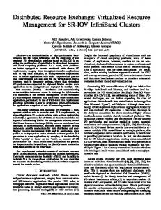
The data center in Figure 1.1 is the top-level resource which cumulatively represents all machines’ resources which are described in Figure 1.2a. In real-life scenarios machines are assigned to nodes, which this thesis will regard as simply another abstraction. Of the resources shown in Figure 1.2a, the bandwidth facilitating vSwitch (Virtual Switch), is denoted as a VM in itself. The vSwitch facilitates local communication between VMs that share a machine, as shown in Figure 1.3a. Outgoing machine traffic taxes both vSwitch and Link resources, where Link is another bandwidth facilitating resource, which is consumed by communication across machines. Communication traffic between machines needs to pass through the vSwitch prior to exiting via a machine Link, as shown 8

1.1 Data Center Architecture

VMs

VMs

Machine 1

Machine 2

Network abstraction which houses Machines.

Source of external traffic. Top-level network abstraction.

Internet

Virtual Machines consume resources.

Compute Node 1

Machine 3

VMs

Compute Node 2

Machine 4

VMs

Data Center

Machines provide resources.

Machine 6

VMs

Machine 5

VMs

Figure 1.1: General data center model employed in this thesis. in Figure 1.3b. Because the vSwitch is essentially a VM it will be regarded as a preexisting resourceconsumer, whose RAM, vCPU, disk consumption has been taken into account prior to a VM placement.

1.1.1 Virtual Network Functions (VNFs) In this thesis VNFs are entities which group VMs together, and describe how those VMs communicate within that group. Communication described by VNF groups obeys a particular network topology, such as Partially Connected Mesh Network Topology Figure 1.4a, or Artificial Neural Network Topology Figure 1.4b. Thesis will focus on the Artificial Neural Network Topology, as it is a simple topology where all VMs evenly distribute traffic amongst themselves.

1.1.2 Virtual Machines (VMs) VMs are elements which consume resources as described in Figure 1.2b. They may also contain placement rules in the form of Affinities and Anti-Affinities, which respectively denote whether certain VMs must be placed on the same physical machine, or must never be placed on the same physical machine. For a particular VM placement to be valid such placement rules must be obeyed. As mentioned in section 1.1, the vSwitch is regarded as a VM itself. Each machine is inherently required to have one vSwitch to facilitate VM communication within a machine. Outgoing machine traffic taxes the vSwitch prior to its exit through Link. vSwitch is the only VM element which may not have any of the aforementioned Anti/Affinity placement rules, as each machine is required to have a vSwitch. It also provides 9

1. Problem Description and Applications

RAM

RAM resources in [MiB].

RAM

RAM consumption in [MiB].

Disk

Disk resources in [MiB].

Disk

Disk consumption in [MiB].

vCPU

# of vCPUs available.

vCPU

# of vCPUs required.

Link

Bandwidth in [Bps] or [PPS].

Affinities

List of VMs belonging to Affinity group.

[VM] vSwitch

Bandwidth in [PPS].

AntiAffinities

List of VMs belonging to Anti-affinity group

(a) Each machine’s resource provision model. The vSwitch is part of a VM which every machine is required to have. A constant enabling conversion between units PPS (Packets Per Second) and Bps is given.

(b) Virtual machine resource consumption model with placement rules. Affinities force VMs to share the same machine, whereas Anti-affinities prohibit VMs from sharing the same machine.

Figure 1.2: Description of VM and Machine models. a bandwidth resource while simultaneously consuming machine resources.

1.2

Placement Algorithm Goals

Given machines with a known amount of available resources (Figure 1.2a), VM elements with known resource consumption (Figure 1.2b), their Anti-/Affinity placement rules (see subsection 1.1.2), and place within the VNF group they belong to (see Figure 1.5b), a placement problem with bandwidth analysis will be solved. With the example placement in Figure 1.5 in mind, an algorithm with the following properties will be proposed: i VM placement that obeys Anti-/affinity placement rules. ii Performs bandwidth analysis once placement is complete. This analysis is done according to the each VNF group’s Artificial Neural Network Topology (see Figure 1.4b). iii VM placement obeys machine resource constraints (RAM, Disk, vCPU). iv Optionally permit usage of a bandwidth objective which placed system must handle (vSwitch, Link).

10

1.2 Placement Algorithm Goals

Machine VM1

VM2

vSwitch

Link (a) Dotted arc denotes simplex communication from VM1 to VM2. Black arcs illustrate how this communication is actually facilitated. Traffic taxes the machine’s vSwitch.

Machine 1

Machine 2 VM1

VM2

vSwitch

vSwitch

Link

Link

(b) Dotted arc denotes simplex communication from VM1 to VM2 across two machines. Black arcs illustrate how the two machines’ vSwitch and Link facilitate this communication. Traffic taxes both machine’s respective Link and vSwitch.

Figure 1.3: An illustration of the discrepancy between how VMs want to communicate (dotted arcs), and which resources machines expend to facilitate simplex communication (black arcs).

11

1. Problem Description and Applications

1.3

Related Work

The foundation to this thesis’ VM placement solution is a packing problem formulation named Knapsack Problem (KP). The methodology described by KP is analogous to packing a real life rucksack, such that items placed inside said rucksack do not exceed its weight and volume limit. Also, the cumulative value of the items placed into the rucksack should have as much value as possible. Less formally, it can be said that a fridge won’t be on the rucksack’s packing list, as it weighs a lot, takes a lot of volume, is not practical, and therefore has almost zero value. However, a map and compass weigh very little, take up small volume, and are very useful, which means they have a great value. Previous work on VM placement algorithms largely employ variants of a packing algorithm named the Multiple Knapsack Problem [1] [10], where aforementioned rucksack analogy is applied just the same, but for several rucksacks, such that cumulative value of items packed into all rucksacks is as large as possible. The most related VM placement work is [3], which employs a Multidimensional Multiple Knapsack Problem model. It similarly implies that several rucksacks are packed, and the cumulative value of all packed items is maximized just like before, however now the rucksacks and items have multiple weights and volumes respectively, thereby making the problem multidimensional. Importantly, [10] showed that hierarchical cloud structures can be represented as placement constraints that are modeled as matrices. In this work a different approach is employed, such that only VM placements are modeled as matrices, whereas the hierarchical cloud structure is maintained by generating constraints which identify how VMs communicate given a placement, such that a bandwidth objective can be met. In order to compensate for certain performance penalties heuristics are employed (see 2.6.2) which avoid searching where there are no solutions. According to [16, p. 5] 2013 VM Placement Literature Review, publication [14] proposes an on-line bandwidth-maximizing VM placement algorithm, which amongst its drawbacks lists significant compute-resource wastage for the purpose of maximizing network utilization. Similarly, the proposed algorithm in this thesis is off-line for the same reason, as bandwidth analysis is a very computationally intensive element. Just as in publication [10] Modeling and Placement of Cloud Services with Internal Structure, this thesis proposes a VM placement with bandwidth analysis, but with a simpler network topology model. However, this an exact bandwidth analysis algorithm as opposed to the 2-approximation algorithm that minimizes traffic between VMs which [10, p.3] proposes. The penalty for using an exact algorithm is longer computation time. Because publication [3] shows that Multiple Multidimensional Knapsack Problem can be used to model the VM placement problem, it follows that fundamental Knapsack Problem’s special case Subset-sum Problem (when item weights and item values are the same) is also suitable as a problem model. Analogously, the Subset-sum Problem’s objective is to fully utilize rucksack capacities by packing as many items as possible. This SubsetSum Problem special case lays the foundation to this thesis’ algorithm, and is discussed in chapter 2.

12

1.3 Related Work

VM7

VM8

VM5

VM4

VM2 VM1 s

VM3

VM3 VM4

VM2

VM6

VM5

(a) Partially Connected Mesh Network Topology. Network traffic from and to s is unevenly distributed amongst VMs through bidirectional arcs.

VM1

VM6

s

(b) Artificial Neural Network Topology. Network traffic from s is evenly distributed amongst all VMs according to a communication hierarchy using directed arcs. This thesis will use a bidirectional arc case, where VM7 and VM8 also would distribute their result downwards in the communication hierarchy, and back to traffic source s.

Figure 1.4: Two main network topologies used to describe VM group communication within a VNF. Figure 1.4a provides a flexible topology with point-to-point connections. Figure 1.4b employs interconnection of VMs similar to a k-partite graph. VNFs are unaware of how this communication will be facilitated by the data center (see Figure 1.3). This thesis focuses on the topology shown in Figure 1.4b.

13

1. Problem Description and Applications

Affinity VM1 VM2 VNF1 VM3

VM4

VNF2 VM1

VM3

VM2

VM4

VM6

VM7

Affinity VM5

VM6

VM5

Anti-Affinity VM7 s

(a) Information regarding placement rules. Each VM may have Affinities, or Antiaffinities towards other VMs (see subsection 1.1.2). In this example all VMs have Anti-/Affinity placement rules.

Machine 1

(b) Information regarding VNF groups which the VMs belong to. Each VNF’s internal communication employs bidirectional Artificial Neural Network Topology, as explained in Figure 1.4b.

Machine 2 VNF1 VM2

VM1

VM7

VM3

VM4

VM5

VM6 VNF2

vSwitch

vSwitch

Link

Link

(c) Resultant placement on two machines. VNF groups have now been scattered across machines due to VM placement. Note how Affinity and Anti-affinity rules from Figure 1.5a are obeyed.

Machine 1

Machine 2 VNF1 VM2

VM1

VM3

VM7

VM4

VM5

VM6 VNF2

vSwitch

vSwitch

Link

Link

s

(d) Communication commences after VM placement. VNF traffic obeys Figure 1.5b description. Dotted bidirectional arcs depict a duplex communication scenario of Figure 1.3.

Figure 1.5: VM placement problem example. Solved with respect to Affinity, Anti-affinity, and VNF groups. 14

Chapter 2 Problem Model

The problem model is built on a subset-sum version of Multidimensional 0/1 Multiple Knapsack Problem (0-1 MMKP), such that knapsacks accommodate three volumes, factor in placement constraints, and placement-dependent bandwidth analysis. Simpler Knapsack variants will be presented prior to the proposed algorithm’s 0-1 MMKP based model.

2.1 0/1 Knapsack Problem (0-1 KP) The 0/1 Knapsack Problem (0-1 KP) is an NP-hard combinatorial optimization problem [6], which throughout the centuries has been found to have applications in cryptography [13], networking [20], economics [7], and scheduling [25]. The formal definition of 0-1 KP [17, p.11] follows: Definition 2.1.1. 0/1 Knapsack Problem: Given n ∈ Z+ items, their item weights wj item profits vj and one knapsack of weight capacity c > 0. Choose a subset of the n items such that the cumulative item profit inside the knapsack is maximized without exceeding the knapsack’s weight capacity c: Maximize: Subject to:

n ∑ j=1 n ∑

v j xj

(2.1)

wj xj ≤ c.

(2.2)

j=1

xj ∈ {0, 1},

j = 1, ..., n,

(2.3)

where xj is a binary variable governing whether item j should be packed into the knapsack. When xj = 1 item is included in the knapsack, and excluded from the knapsack when xj = 0. 15

2. Problem Model as Combinatorial Optimization

2.2

0/1 Multiple Knapsack Problem (0-1 MKP)

Due to the nature of 0-1 KP it can be scaled up to multiple knapsacks, which then becomes the 0/1 Multiple Knapsack Problem (0-1 MKP), which is an NP-hard problem. 0-1 MKP permits more complex problem formulations than 0-1 KP, and has applications in radar technology [11], Cloud systems [1][5], multiprocessor scheduling [4], and energy management [18]. The formal definition of 0-1 MKP [17, p.13] follows: Definition 2.2.1. 0/1 Multiple Knapsack Problem: Given n ∈ Z+ items, their item weights wj item profits vj and m ∈ Z+ knapsacks of weight capacities ci . Choose a subset of the n items such that the cumulative item profit inside each knapsack is maximized without exceeding each knapsack’s weight capacity cj : Maximize: Subject to:

m ∑ n ∑

(2.4)

vj xij

i=1 j=1 n ∑

wj xij ≤ ci ,

i = 1, ..., m,

(2.5)

xij ≤ 1,

j = 1, ..., n,

(2.6)

xij ∈ {0, 1},

i = 1, ..., m,

j=1 m ∑ i=1

j = 1, ..., n.

(2.7)

Here xij = 1 indicates that item j should be packed into knapsack i, and Equation 2.5 ensures that capacity constraint of each knapsack is satisfied. Constraint Equation 2.6 ensures that each item is chosen at most once. Remark (Subset-sum Problem). A special case in Definitions 2.1.1, 2.2.1 when wj = vj [21, p.2] is termed as the Subset-Sum Problem, and Multiple Subset-Sum Problem respectively [17, p.157]. Their objective is to find a subset of items whose sum is closest to, but not exceeding, knapsack capacity. Mentioned subset-sum case in Definition 2.2’s remark is particularly important to this thesis, as it will be used to compute RAM, vCPU, disk consumption in machines.

2.3

Multidimensional Multiple Subset-Sum Problem (MDMSSP)

By using 0-1 MKP special case where wj = vj (see Definition 2.2’s remark) a Multiple Subset-Sum Problem (MSSP) is formulated. In order to facilitate a problem model accounting for machine three resources (RAM, vCPU, disk), items will need several weights, and knapsacks several capacities. Therefore MSSP will be scaled up to a Multidimensional Multiple Subset-Sum Problem (MDMSSP): Definition 2.3.1. Multidimensional Multiple Subset-Sum Problem: Given d ∈ Z+ dimensions and n ∈ Z+ items, their item weights wjr and m ∈ Z+ knapsacks of weight 16

2.4 Proposed Problem Model

capacities cir . Choose a subset of the n items such that the cumulative item weights inside each knapsack is maximized without exceeding each knapsack’s weight capacities cir :

Maximize:

m ∑ n d ∑ ∑

(2.8)

wjr xij

r=1 i=1 j=1

Subject to:

d ∑ n ∑

wjr xij ≤ cir ,

i = 1, ..., m,

(2.9)

xij = 1,

j = 1, ..., n,

(2.10)

xij ∈ {0, 1},

i = 1, ..., m,

r=1 j=1 m ∑ i=1

j = 1, ..., n.

(2.11)

Here xij = 1 indicates that item j should be packed into knapsack i, whereas Equation 2.9 ensures that the d different capacities of each knapsack are satisfied. Constraint Equation 2.10 denotes that each item must be packed. A simple VM placement problem can be modeled with MDMSSP. When dimensions d = 3 each dimension refers to the resources RAM, vCPU, and disk resources. Resultant item weights would represent VM resource consumption, whereas knapsack capacities would be machine resources.

2.4 Proposed Problem Model Building upon the MDMSSP combinatorial problem model described in section 2.3 additional constraints will be supplemented to factor in VM Anti-/Affinity placement restriction rules (see subsection 1.1.2), and bandwidth resource constraints in Link and vSwitch. Bandwidth constraints are modeled such that for each MDMSSP knapsack in section 2.3 two new knapsacks will be created, whose capacities are governed by Link and vSwitch bandwidth resources present in each machine. During bandwidth analysis, if a traffic edge spans across machines, then both machines’ vSwitch and Link are consumed (Figure 1.3b). Whereas, if an edge resides within one machine, only that machine’s vSwitch is consumed (Figure 1.3a). The following will build on the MDMSSP Definition 2.3.1, with modifications to accommodate for Anti-/Affinity placement restrictions rules (see subsection 1.1.2), and VNF groups that specify how VMs distribute traffic amongst themselves (see Figure 1.5b). Definition 2.4.1. Multidimensional Multiple Subset-Sum Problem with item placement restrictions and bandwidth analysis: Given d ∈ Z+ dimensions and n ∈ Z+ items, their item weights wjr and m ∈ Z+ knapsacks of weight capacities cir . Choose a subset of the n items such that the cumulative item weights inside each knapsack is maximized without 17

2. Problem Model as Combinatorial Optimization

exceeding each knapsack’s weight capacities cir : Maximize:

d ∑ m ∑ n ∑

(2.12)

wjr xij

r=1 i=1 j=1

Subject to:

d ∑ n ∑

wjr xij ≤ cir ,

i = 1, ..., m,

(2.13)

xij = 1,

j = 1, ..., n,

(2.14)

xij ∈ {0, 1}.

i = 1, ..., m,

r=1 j=1 m ∑ i=1

j = 1, ..., n,

(2.15)

xij = 1 indicates that item j should be packed into knapsack i, and Equation 2.13 ensures that the d different capacities of each knapsack are satisfied. Constraint Equation 2.14 denotes that each item must be packed. An item j may optionally have placement restrictions, such that it must not share knapsack with another item q. Similarly, there’s an optional placement restriction, such that an item j must share knapsack with another item q. For each such item j with a placement rule towards an item q following constraints are formulated: Anti-affinities: xij = 1 =⇒ xij ̸= xiq Affinities: xij = 1 =⇒ xij = xiq

i = 1, ..., m, q = 1, ..., n, i = 1, ..., m, q = 1, ..., n,

j j j j

= 1, ...n, ̸= q, (2.16) = 1, ..., n, ̸= q. (2.17)

Let there be a known g ∈ Z+ amount of VNFs denoted as graphs Gp = (Ep , Vp , Ω, s), such that p = 1, ..., g. Each graph Gp has a known k ∈ Z+ amount of layered groups denoted Lp,l , such that the amount of layered groups is Gp graph specific. It is also known to which layered group Lp,l each of the j = 1, ..., n packed items belong to, such that ∃j ∈ Lp,l . Thereby making each item j a vertex, such that ∀j ∈ Vp . Let there be a traffic source s generating an unknown amount of traffic t ∈ Z+ . Edges’ (j, q) ∈ Ep weight ωiq ∈ Ω is directly dependent on traffic t originating from s, where j = 1, ..., n and q = 1, ..., n. The edge weight relation depends on how many items there are on previous layered groups, such that distributive traffic is employed as shown in Equation 2.22. Edges (s, p) ∈ Ep between s and all items p ∈ Lp,1 , which is the layered group whose layer is l = 1 are formed. Traffic t originating from s is thereby evenly distributed between items in p layered groups Lp,1 . Within each individual Gp even distribution of traffic between each layered group’s items occurs, all the way to the top layered group Lp,max(k) , where max(k) ∈ Gp . Let there be two known additional capacities to each knapsack denoted ci,d+1 and ci,d+2 which represent vSwitch and Link resources respectively. Let there also be a known bandwidth objective b ∈ Z+ .

18

2.4 Proposed Problem Model

G1 L1,1 V3 V2 V1

L1,2

L1,3

V8 V7 V6 V5 V4

V11 V10 V9

L2,2

L2,3

V15 V14 V13

V18 V17 V16

s G2 L2,1 V12

L2,4 V19

Figure 2.1: Example of graphs Gp = (Vp , Ep , Ω, s), where each arc represents an edge e with a weight ω(e) that is directly related to traffic t originating from s. Bandwidth analysis problem is defined in full by constraints in equations 2.18-2.23, which if satisfied, imply that placed system handles bandwidth objective b. t ≥ b, where t is unknown, g max(k)−1 ∑ ∑ ∑ p=1

+

ωjq · tijiq +

g max(k)−1 ∑ ∑ ∑ p=1

j∈Lp,l q∈Lp,l+1

l=1

g n ∑ ∑

∑

(2.18)

l=1

ωsj · xij ≤ ci,d+1 , for all Lp,k ∈ Gp ,

∑

ωiq · tijzq

j∈Lp,l q∈Lp,l+1

i = 1, ..., m,

z = 1, ..., m,

(2.19)

i = 1, ..., m,

z = 1, ..., m,

(2.20)

p=1 j=1

∑ max(k)−1 ∑ ∑ g

p=1

ωjq · tijzq

j∈Lp,l q∈Lp,l+1

l=1

n ∑∑

∑

g

+

ωsj · xij ≤ ci,d+2 , for all Lp,k ∈ Gp ,

p=1 j=1

tijzq = xij ∧ xzq , where i = 1, ..., m, j = 1, ..., n, z = 1, ..., m, q = 1, ..., n, x ∈ {0, 1} t ωjq = l+1 , where j = 1, ..., n, q = 1, ..., n, ∏ ∑g |Lp,f | · p=1 |Lp,1 |

(2.21) (2.22)

f =1

ωsj = ∑g

t

p=1

|Lp,1 |

, where j = 1, ..., n.

(2.23)

To test whether traffic travels inside or across machines Equation 2.21 performs boolean operation on the placement variables x ∈ {0, 1}, whose result is 1 if such communication occurred. Equation 2.21 tests for communication on same machine for tijiq and across machines for tijzq . To cover the case of vSwitch consumption Equation 2.19 does a cumulative sum of knapsack placement possibilities where edges go across knapsacks, and within existing 19

2. Problem Model as Combinatorial Optimization

knapsacks, such that vSwitch capacity ci,d+1 is honored. Link consumption calculated by Equation 2.20 performs the same calculation, but only takes edges going across knapsacks into account, such that Link capacity ci,d+2 is honored. Equation 2.22 defines that items within layered groups Lp,l employ distributive traffic, whereas Equation 2.23 defines that traffic t originating from vertex s is evenly distributed amongst items j in layered groups adjacent to s. This concludes the definition of the proposed Multidimensional Multiple Subset-Sum Problem with item placement restrictions and bandwidth analysis.

2.5

Discarded Problem Models

This thesis’ initial approach to the VM placement problem was a hypergraph partitioning problem model. Inspired by Prof. Ümit V. Çatalyürek’s work on hypergraph partitioning [8], the intent was to model VMs as vertices, and machines as hypervertices. Weights would be attributed to directed edges in the hypergraph to denote communication costs, and additional weights to both vertices and hypervertices to denote consumption various resources. Due to the difficulties of modeling how arc weights are denoted depending on the entities they pass (machines) on their way to their target, and whether the edge consumes a machine’s Link and vSwitch or only vSwitch, it was difficult to employ High Performance Computing (HPC) hypergraph partitioning libraries to attack this problem. The model was discarded, as amount of different weight variables required by this particular VM placement could not be facilitated by HPC hypergraph partitioners.

2.6

JaCoP Constraint Problem Solver

This section serves as a short introduction to constraint programming, and the features used to implement this thesis’ proposed VM placement algorithm. Combinatorial problem model defined in 2.4.1 is expressed in terms of the Java Constraint Problem Library (JaCoP). A library implemented by Prof. Krzysztof Kuchcinski and PhD. Radosław Szymanek, which received a bronze medal in the annual competition of constraint programming solvers MiniZinc Challenge 2015 [22]. JaCoP facilitates integer, floating-point, logical, and set constraints, [15] of which integer constraints were chosen for solving this particular VM placement problem. Packing of VMs on machines is implemented through weighted sums of Finite Domain Variables (FDV)[15, p.11], which denote unknown variables whose value is restricted by an integer domain. For example, a FDV X can be restricted to values within domain X::[1..5]. This property is used to let VMs consume machine resources up to a specific machine resource’s upper integer domain limit. Similarly, traffic edge weight FDVs can be created with successively smaller domains, such that search-space is reduced in a safe way.

2.6.1

Introduction by Sudoku example

Permit the premise that constraint programming can solve a Sudoku problem. The objective is to fill a 9 × 9 grid with numbers ranging 1, ..., 9, such that each column, row, and 20

2.6 JaCoP Constraint Problem Solver

Indomain method IndomainMin IndomainMax IndomainMiddle IndomainRandom IndomainSimpleRandom IndomainList IndomainHierarchical

Description selects a minimal value from the current domain of FDV selects a maximal value from the current domain of FDV selects a middle value from the current domain of FDV and then left and right values selects a random value from the current domain of FDV faster than IndomainRandom but does not achieve uniform probability uses values in an order provided by a programmer uses indomain method based provided variable-indomain mapping

Table 2.1: Value Selection Heuristics. Cited from JaCoP documentation [15, p.83]. the nine 3 × 3 boxes are restricted to contain unique numbers. Since each cell inside the grid may only contain the numbers 1, ..., 9, the cells are suitable to be expressed as Finite Domain Variables with domains [1,..,9], which corresponds to the integers permitted by the rules of Sudoku. JaCoP constraint programming library provides a readily applicable constraint named alldifferent([x1, x2, . . . , xn]) which in this case would cause the FDVs to be different within their permitted domains [1,..,9]. What follows is the vectorization of each row, column, and 3 × 3 box such that the constraint may be imposed. After imposing alldifferent constraint the Sudoku problem has been successfully modeled, and a solution space has been thereby defined. By searching within the defined solution space using a Depth First Search a set of correct solutions can be found. In this thesis however, the focus is obtaining just one solution. Behavior of the Depth First search can be altered using several heuristics provided by the JaCoP library.

2.6.2 Search Heuristics JaCoP facilitates tools for defining own search methods, by modifying existing ones, through search-plugins [15, p.49]. In the presented solution, only a subset of the variables used in 2.4.1 are part of the search. Employed search method builds on a Depth First Search (DFS), which organizes the search-space into a search tree [15, p.49]. Every node within the search tree is subject to become a choice point, where FDVs chosen by a variable selection heuristic Table 2.2 are assigned a value by a value selection heuristic Table 2.1. Subsequent constraint propagation is triggered once a FDV has been assigned a value. Should a constraint not be satisfied during this constraint propagation, then search is cut at that point in the tree, thereby preventing searching sub-trees where there are no solutions. Chosen variable selection heuristic is MostConstrainedDynamic, which is motivated by how constraints on FDVs pile up during bandwidth analysis, which figuratively becomes a red thread which the MostConstrainedDynamic variable selection heuristic in Table 2.2 can follow. However, this does not mean MostConstrainedDynamic is the best variable selection heuristic, as SmallestDomain variable selection heuristic outperforms MostConstrainedDynamic when there are few VM placement constraints. In order to minimize computation time a hierarchical heuristic was chosen, such that each FDV can be subjected to a different value selection heuristic. The motivation behind 21

2. Problem Model as Combinatorial Optimization

Comparator SmallestDomain MostConstrainedStatic MostConstrainedDynamic SmallestMin SmallestMax LargestDomain LargestMin MaxRegret WeightedDegree

Description selects FDV which has the smallest domain size selects FDV which has most constraints assigned to it selects FDV which has the most pending constraints assign to it selects FDV with the smallest value in its domain selects FDV with the smallest maximal value in its domain selects FDV with the largest domain size selects FDV with the largest value in its domain selects FDV with the largest difference between the smallest selects FDV with the highest weight divided by its size

Table 2.2: Variable Selection Heuristics. Cited from JaCoP documentation [15, p.83]. this is because VM placement variables are an m × n logical matrix, whose element’s domains are [0..1]. Bandwidth variables on the other hand are positive integers with domains typically reaching [0..10000]. Because of this FDVs related to bandwidth do not benefit from being treated with the same variable selection heuristic [15, p.83]. More specifically, important variables consist of the following heuristics which act on the solution-search tree: • 0/1 Placement Matrix FDVs: IndomainRandom. Perhaps a counterintuitive choice of value selection heuristic, as IndomainMax would cause a VM to be placed immediately. However, using IndomainMax skews the VM placement. Because the [0..1] domains residing in the placement matrix will be immediately assumed to be 1, and because the matrix traversal is iterative, some machines become more heavily utilized than others, which is why IndomainRandom is preferred. Therefore it can be said that IndomainRandom produces a more balanced VM placement. • Incoming VNF traffic FDVs: IndomainMax. Incident traffic is not maximized, however should always be as large as possible even when the optional bandwidth objective is not used. • Communicating VMs not sharing machine variable: IndomainMin. This FDV is the boolean result of a Reified constraint [15, p.74] which is true when two VMs do not share a machine. Because VMs communicating across machines can be detrimental to IaaS Cloud performance, the value selection heuristic will always assume this value is false. • Communicating VMs sharing machine FDVs: IndomainMax. This FDV is the boolean result of a Reified constraint [15, p.74] which is true when two VMs share a machine. VMs communication within machines is more preferred than VMs communicating across machines. The value selection heuristic will always assume this value is true. • Cumulative bandwidth into VNFs FDVs: IndomainMax. Selects the maximum integer value permitted by FDV’s domain, such that incident traffic into Cloud can be as large as possible. This does not maximize bandwidth, only selects the largest value. 22

2.6 JaCoP Constraint Problem Solver

• All above mentioned FDVs: IndomainHierarchical. Individually attributed value selection heuristics for all previously mentioned FDVs is made possible by supplying the attributes with IndomainHierarchical. This value selection heuristic provides variable-indomain mapping by supplying indomain methods using a Java HashMap. • All other FDVs: IndomainRandom. This is the default value selection heuristic for all variables which the IndomainHierarchical value selection heuristic does not supply an indomain method for. Essentially unused because all variables already have an indomain method supplied using IndomainHierarchical. Traffic across machines is more undesirable than traffic within machines, which is imposed by attributing IndomainMax value selection heuristic to traffic arcs between VMs within one machine, and IndomainMin to traffic arcs for VMs communicating across machines. To summarize, MostConstrainedDynamic variable selection heuristic, and above listed value selection heuristics are employed by the Depth First Search (DFS) based restart-search seen in Listing 2.1, from which no-good elements are derived, such that every restart contributes with new no-goods. Search is run until one solution is found. If no solution is found, or solution-space is exhausted, then the entire search routine fails. Upon failure an assumption is made, that the failure is due to lack of machines to place VMs on, and search procedure is promptly restarted with an extra machine, which thereby expands the search-space. It is important to mention that only a certain subset of FDV variables have been deemed suitable to become selection points within the DFS search tree. Theoretically however, every FDV within the problem model could be explicitly treated with a different value selection heuristic. Whether this is something desirable has not been investigated, but will be discussed later in chapter 4.

23

2. Problem Model as Combinatorial Optimization

1 /** 2 * I t c o n d u c t s t h e s e a r c h w i t h r e s t a r t s from which t h e no−g o o d s a r e d e r i v e d . 3 * E v e r y s e a r c h c o n t r i b u t e s w i t h new no−g o o d s which a r e k e p t s o e v e n t u a l l y 4 * t h e s e a r c h i s c o m p l e t e ( a l t h o u g h c a n be v e r y e x p e n s i v e t o m a i n t a i n e x p l i c i t l y 5 * a l l no−g o o d s f o u n d d u r i n g s e a r c h ) . Employs I n d o m a i n H i e r a r c h i c a l which u s e s 6 * t h e i n d o m a i n method s p e c i f i e d by a v a r i a b l e −i n d o m a i n mapping . 7 * 8 * @return t r u e i f t h e r e i s a s o l u t i o n , f a l s e o t h e r w i s e . 9 */ 10 11 p u b l i c b o o l e a n s e a r c h W i t h R e s t a r t s H i e r a r c h i c a l ( ) { 12 13 /* immediate f a i l c o n d i t i o n */ 14 i f ( f a i l == t r u e ) 15 return false ; 16 17 /* i n i t i a l i z e */ 18 boolean r e s u l t = f a l s e ; 19 boolean timeout = t r u e ; 20 21 / * D e f i n e DFS s e a r c h * / 22 s e a r c h = new D e p t h F i r s t S e a r c h < I n t V a r > ( ) ; 23 24 / * employ M o s t C o n s t r a i n e d D y n a m i c FDV v a r i a b l e s e l e c t i o n h e u r i s t i c , and */ 25 / * I n d o m a i n H i e r a r c h i c a l v a l u e s e l e c t i o n h e u r i s t i c which s u p p l i e s i n d o m a i n * / 26 / * mapping f o r e a c h FDV i n d i v i d u a l l y . F a l l b a c k t o IndomainRandom v a l u e */ 27 / * s e l e c t i o n h e u r i s t i c f o r FDVs which I n d o m a i n H i e r a r c h i c a l d o e s n o t */ 28 / * s p e c i f i y i n d o m a i n mapping f o r . */ 29 S e l e c t C h o i c e P o i n t < I n t V a r > s e l e c t = new S i m p l e S e l e c t < I n t V a r > ( 30 v a r s . t o A r r a y ( new I n t V a r [ 1 ] ) , new M o s t C o n s t r a i n e d D y n a m i c < I n t V a r > ( ) , 31 new I n d o m a i n H i e r a r c h i c a l < I n t V a r > ( h i e r a r c h i c a l M a p , new IndomainRandom < I n t V a r > ( ) ) ) ; 32 33 / * p r e p a r e no−g o o d s c o l l e c t i o n * / 34 N o G o o d s C o l l e c t o r < I n t V a r > c o l l e c t o r = new N o G o o d s C o l l e c t o r < I n t V a r > ( ) ; 35 search . setExitChildListener ( collector ) ; 36 search . setTimeOutListener ( collector ) ; 37 search . setExitListener ( collector ) ; 38 39 /* search with r e s t a r t s */ 40 while ( timeout ) { 41 search . setPrintInfo ( false ) ; 42 / * r e s t a r t s e a r c h a f t e r 1000 n o d e s * / 43 search . setNodesOut (1000) ; 44 r e s u l t = search . labeling ( store , select ) ; 45 t i m e o u t &= c o l l e c t o r . t i m e O u t ; 46 47 /* prepare for search r e s t a r t */ 48 s e a r c h = new D e p t h F i r s t S e a r c h < I n t V a r > ( ) ; 49 c o l l e c t o r = new N o G o o d s C o l l e c t o r < I n t V a r > ( ) ; 50 search . setExitChildListener ( collector ) ; 51 search . setTimeOutListener ( collector ) ; 52 search . setExitListener ( collector ) ; 53 } 54 return result ; 55 }

Listing 2.1: Solution search routine employed. Builds on restartsearch with no-goods collection.

2.6.3

Implementation

This section serves as an overview of the JaCop implementation stated in 2.4.1. Input to this implementation consists of manually defined machine sizes, and variably specified VMs, Link, and vSwitch, which can be seen in Appendix A. Primary constraints employed are linear integer constraints [15, p.22], which ensure that knapsack capacities are never exceeded. Linear integer constraints are a weighted sums being constrained by a FDV value which relates to one of the operators: , ≥, =. For affinities and anti-affinities conditional constraints are employed, which have the nature IfThen(constraint1, constraint2), where constraint1 would typically express a placement-matrix equality statement, and thereby dynamically impose constraint2 if satisfied. The bandwidth analysis part of procedure 2 is structured such that all possible edge weights are added to a Link and vSwitch ArrayList respectively, where IntVar stands for a FDV. The value of each edge depends on whether traffic actually occurred according to placement, which is decided by the result of tijzq (See Equation 2.21), 24

2.6 JaCoP Constraint Problem Solver

whose behavior is implemented with an AndBool constraint. This means that the summation of each Link & vSwitch knapsack is mostly trailing zeros, among which a few are edges carrying traffic. Therefore it can also be said that implementation of Procedure 2 exploits the fact that constraints can be applied to arrays of dynamic size. Procedure 1 MDMSSP Placement 1: function MDMSSP(m, n, d, xm,n , wn,d , cn,d , Affinities, Anti-Affinities) 2: m ← m amount of Machines 3: n ← n amount of VMs 4: d ← d amount of different knapsack volumes 5: xm,n ← 0/1 placement matrix of size m × n 6: wn,d ← n item weights with d weight categories 7: cn,d ← n knapsacks with d volumes 8: for j = 1 to n do ∑ 9: impose constraint ni=1 xi,j = 1 ◃ Each VM must be placed once. 10: 11: 12: 13: 14: 15: 16: 17: 18:

for r = 1 to d do for i = 1 to m do ∑ ◃ Honor knapsack impose constraint nj=1 wj,r · xi,j − ci,r ≤ ci,r capacities. for each item j which has Affinity to an item q where j, q ∈ n and j ̸= q do for i = 1 to m do impose conditional constraint if xi,j = 1 then xi,j = xi,q for each item j which has Anti-Affinity to an item q where j, q ∈ n and j ̸= q do for i = 1 to m do impose conditional constraint if xi,j = 1 then xi,j ̸= xi,q

25

2. Problem Model as Combinatorial Optimization

Procedure 2 Bandwidth Analysis 1: function BWA(m, n, xm,n , g, p, Lg,p , Vp , Ep , Ω, s, Lm , Sm , t, b) 2: m ← m amount of Machines 3: n ← n amount of VMs 4: xm,n ← 0/1 placement matrix of size m × n 5: g ← g amount of VNFs 6: l ← l amount of layered groups in a VNF 7: Lg,k ← k layered groups in g graphs, where k is VNF-specific max(k) ∈ Gp 8: Ω ← set of edge weights (see 2.22,2.23) 9: s ← traffic source vertex 10: t ← unknown traffic generated by vertex s 11: b ← bandwidth objective 12: Gp ← (Vp , Ep , Ω, s) all VNFs 13: Lm ← m amount of Link knapsacks 14: Sm ← m amount of vSwitch knapsacks 15: L′m,x ← x amount of usages of m Links, where x is of unknown size ′ 16: Sm,y ← y amount of usages of m vSwitches, where y is of unknown size 17: for p = 1 to g do 18: for l = 1 to k − 1, where max(k) ∈ Gp do 19: for j = 1 to n do 20: for q = 1 to n do 21: for i1 = 1 to m do 22: Si′1 ,y+1 ← ωsj · xi1 j ◃ Traffic from s. ′ 23: Li1 ,x+1 ← ωsj · xi1 j ◃ Traffic from s. ′ 24: Si1 ,y+1 ← ωjq · ti1 ji1 q ◃ VM traffic within machines consuming vSwitch. See Equation 2.21. 25: for i2 = 1 to m do 26: Si′1 ,y+1 ← ωjq · ti1 ji2 q ◃ VM traffic across machines consuming vSwitch. See Equation 2.21. ◃ VM traffic across machines 27: L′i1 ,x+1 ← ωjq · ti1 ji2 q consuming Link. See Equation 2.21. 28: for i = 1 to m do ∑ 29: impose constraint max(x) L′i,x ≤ Li ◃ Honor Link knapsack capacities. ∑x=1 max(y) ′ 30: impose constraint y=1 Si,y ≤ Si ◃ Honor vSwitch knapsack capacities. 31:

26

impose constraint t ≥ b

◃ Meet bandwidth objective b.

Chapter 3 Results

Because this work is based on a model whose quality, at this point, is unknown identification of placement quality has been a priority. It can be therefore said that work related to the validation of the presented VM placement model is beyond the scope of this thesis. Thus, placement quality is evaluated. Results are presented in two parts. One dedicated presenting the VM placement algorithm, and the other presenting VM placement with bandwidth analysis. A predefined set of VMs are going to be placed in a predefined set of datacenters found in Table 3.1 and Table 3.2. The vSwitch is a preexisting resource consumer, whose resource consumption is specified in Table 3.1. These placements will not be subjected to affinity and anti-affinity placement restriction rules, as such placements would essentially be predefined, which would hinder an evaluation case where the placement algorithm, and heuristic search algorithm, have free reign.

27

3. Results

Table 3.1: VM resource requirement metrics. VM size vCPU [# cores] RAM [MB] Disk [MB]

Small Medium

Large XLarge XXLarge vSwitch

2 512 1024

6 2048 3072

4 1024 2048

8 4096 8192

12 8192 16384

2 32 512

Table 3.2: Datacenter configurations. Where Datacenter #1 is populated with Small Machines, whereas Datacenters #2,#3 house Medium Machines. See Table 3.3. Datacenter

#1 #2

#3

Small Medium Large XLarge XXLarge

4 2 1 1 0

6 4 2 2 2

8 8 4 4 4

Total [# VMs]

8

16

28

Table 3.3: Machine resource configuration. 1 PPS = 650Bps. Machine

vCPU [# cores]

RAM [MB]

Disk [GB]

vSwitch [PPS]

Link [PPS]

Small Machine Medium Machine

32 32

8192 16384

50 50

50000 50000

100000 100000

28

3.1 Placement Quality

3.1 Placement Quality 3.1.1 Testing methodology Proposed placement algorithm will be evaluated by introducing 3 different datacenter configurations, which will be comprised of VMs in Table 3.1. Datacenter configurations are shown in Table 3.2, inside which VMs are placed on machines seen in Table 3.3. The machines differ only in RAM size, which is motivated by the necessity of keeping machines small enough for the placement algorithm to make decisions, but big enough to house the largest VM specified in Table 3.1. Because the proposed algorithm will always look for solutions where VMs fit on minimal amount of machines, it is important to look at the quality of those solutions. This will be evaluated on VNF groups, which house VMs that do not have any placement restriction rules. Quality of a solution is determined by how evenly resource consumption is distributed across machines, given that the placement algorithm has received free reign due to the lack of affinity, and anti-affinity placement restrictions.

3.1.2 Results Table 3.4: Geometric mean machine of % resource consumption in Datacenter #1 placement when placed on Small Machines (see Table 3.3). Table represents average resource consumption for 30 consecutive placements, and their approximate deviations. Values are: geometric mean ± standard deviation. Datacenter #1 Small Machine 0

Small Machine 1

0.5745 ± 0.2012 0.4739 ± 0.1268 0.1763 ± 0.0618

0.6127 ± 0.2012 0.4933 ± 0.1268 0.1867 ± 0.0618

RAM [%] vCPU[%] Disk[%]

Table 3.5: Geometric mean of % machine resource consumption in Datacenter #2 placement when placed on Medium Machines (see Table 3.3). Table represents average resource consumption for 30 consecutive placements, and their approximate deviations. Values are: geometric mean ± standard deviation. Datacenter #2 Medium Machine 0 Medium Machine 1 RAM [%] vCPU[%] Disk[%]

0.6026 ± 0.1472 0.8958 ± 0.1061 0.3678 ± 0.099

0.7721 ± 0.1276 0.8593 ± 0.1135 0.4881 ± 0.0835

Medium Machine 2 0.7809 ± 0.104 0.8927 ± 0.0955 0.4916 ± 0.0705

29

3. Results

Table 3.6: Geometric machine of % resource consumption in Datacenter #3 placement when placed on Medium Machines (see Table 3.3). Table represents average resource consumption for 30 consecutive placements, and their approximate deviations. Values are: geometric mean ± standard deviation. Datacenter #3 RAM [%] vCPU[%] Disk[%]

3.1.3

Medium M. 0

Medium M. 1

Medium M. 2

Medium M. 3

0.5284 ± 0.0513 0.5428 ± 0.0909 0.8328 ± 0.097 0.8038 ± 0.0763 0.979 ± 0.0438 0.9229 ± 0.0806 0.9376 ± 0.0596 0.7934 ± 0.1048 0.304 ± 0.0269 0.3515 ± 0.074 0.5084 ± 0.0788 0.512 ± 0.0331

Medium M. 4

Medium M. 5

0.7648 ± 0.1015 0.6918 ± 0.1325 0.4805 ± 0.054

0.7557 ± 0.0849 0.7076 ± 0.11 0.4891 ± 0.05

Discussion

The most vital resource vCPU, and RAM are relatively spread in the cases in Table 3.4 and Table 3.5. Congestion in vCPU availability in Table 3.6 made the placement algorithm skew the VM placement, such that Machines 0 through 2 have a greater vCPU load than Machines 4 and 5. Despite the placement matrix being treated with an IndomainRandom heuristic, there is still some bias. The order of the FDV variables in the placement matrix dictate the order of evaluation. Bias becomes apparent as vCPU usage is appears to be descending when seen from left, to right, where left is Machine 0 and right is Machine 5. Incidentally, the vCPU capacity constraint is also the first capacity checked for validity upon VM placement, as it’s regarded as the most vital one. Thereby the order of FDV evaluation plays a role in how balanced a placement is, which is a behaviour stemming from the chosen search heuristic.

30

3.2 Placement with Bandwidth Analysis

VNF1 S

S

S

S

VNF1 S

VNF2 M

S

S

M

M

XL

XL

S VNF2

M L

S

S

S

S

XXL

XXL

XL

s

s

(a) Datacenter #1 network topology being employed during bandwidth analysis. VNF1

(b) Datacenter #2 network topology being employed during bandwidth analysis.

VNF2 S

S

S

S

S

S

S

S

M

M

S VNF3

M

M

XL

M

XL

XXL

M

XL

XXL

XL

XXL

S

S

M

S

M

XXL

s

(c) Datacenter #3 network topology being employed during bandwidth analysis.

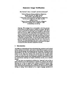
Figure 3.1: Datacenters and their respective VNF groups during placement with bandwidth analysis. Notation: S,M,XL,XXL refer to VMs of size denoted in Table 3.1. Node s refers to a source of traffic, and can be regarded as the internet.

3.2 Placement with Bandwidth Analysis 3.2.1 Testing Methodology Datacenters’ VMs in Table 3.2 will be put in particular network configurations show in Figure 3.1. Placement commence without a bandwidth objective, then with a bandwidth objective. Network resources are taxed as previously stated in Figure 1.3. As mentioned in the beginning of this chapter, affinity and anti-affinity placement restriction rules will not apply for these placements, such that the quality of the placement can be evaluated.

31

S

S

3. Results

3.2.2

Results Table 3.7: Placement with bandwidth analysis of Datacenter #1 when bandwidth is not maximized. Values are: geometric mean of percentage utilization ± standard deviation. Datacenter #1

Small Machine 0

Small Machine 1

RAM [%] vCPU [%] Disk [%] Link [%] vSwitch [%]

0.6617 ± 0.208 0.5133 ± 0.1166 0.2019 ± 0.0658 0.3764 ± 0.0876 0.954 ± 0.1215

0.5213 ± 0.208 0.4595 ± 0.1166 0.1587 ± 0.0658 0.342 ± 0.2032 0.8501 ± 0.0618

External traffic [PPS] 31403 ± 13686.78

Table 3.8: Placement with bandwidth analysis of Datacenter #1 when bandwidth is maximized. Values are: percentage resource utilization. Datacenter #1

Small Machine 0

Small Machine 1

RAM [%] vCPU [%] Disk [%] Link [%] vSwitch [%]

0.3137 0.2667 0.0808 0.5 1

0.9411 0.7334 0.3030 0.2083 1

External traffic [PPS]

62502

Table 3.9: Placement with bandwidth analysis of Datacenter #2 when bandwidth is not maximized. Values are: geometric mean of percentage utilization ± standard deviation. Datacenter #2

Medium Machine 0 Medium Machine 1

RAM [%] vCPU[%] Disk[%] Link [%] vSwitch [%]

0.7629 ± 0.1373 0.9646 ± 0.0625 0.4717 ± 0.0894 0.3252 ± 0.0988 0.7959 ± 0.2333

External traffic [PPS]

23748 ± 3651.48

32

0.7508 ± 0.139 0.9014 ± 0.1128 0.4733 ± 0.0906 0.2425 ± 0.1227 0.5265 ± 0.2904

Medium Machine 2 0.631 ± 0.1578 0.7834 ± 0.1144 0.3963 ± 0.1044 0.236 ± 0.1381 0.5232 ± 0.3182

3.2 Placement with Bandwidth Analysis

Table 3.10: Placement with bandwidth analysis of Datacenter #2 when bandwidth is maximized. Values are: percentage resource utilization. Datacenter #2

Medium Machine 0 Medium Machine 1

RAM [%] vCPU[%] Disk[%] Link [%] vSwitch [%]

0.7514 0.9333 0.4848 0.3758 0.9523

External traffic [PPS]

45092

0.7828 1 0.4646 0.35 1

Medium Machine 2 0.6575 0.7333 0.4242 0.3759 0.8018

3.2.3 Discussion Bandwidth analysis in Table 3.7 without a bandwidth objective portrays a great deviation in found handleable duplex traffic. Once given a bandwidth objective as seen in Table 3.8 it finds very good solutions for small systems. There is a high chance that the solution in Table 3.8 is a global optimum, as vSwitch is completely exhausted on both machines. None of the machine’s resources are overloaded, however a great margin of resource balance has been sacrificed to meet the bandwidth objective, which is clearly observed in Machine 1’s 94% RAM consumption, which is a contrast to Machine 0’s 31% RAM consumption. Algorithm’s primary objective has become bandwidth, and resource consumption is now secondary. Despite maximizing bandwidth in Table 3.10 the external traffic value is not as high as in Table 3.8, which speaks for room for improvement in the solution search heuristic. Tailoring heuristics for VM placement and VM placement with bandwidth analysis separately would likely lead to much better solutions. Such tailoring could be applied for communication edges with rules which govern probability of an edge leading to a functioning placement. Because bandwidth analysis generates a lot more constraints, previously tested Datacenter #3 could not be analyzed for bandwidth, and will be regarded as a timeout. However could be evaluated in the future if a computer with enough RAM is facilitated for testing.

33

3. Results

34

Chapter 4 Conclusion

As stated in chapter 3 this work builds on a model whose quality is unknown, and its evaluation will be listed as future work. All material is presented such that it obeys Ericsson NDA. Also, validation of the VM placement model is beyond the scope of this thesis. In summary, the proposed VM placement algorithm has built on an NP-hard (0/1 Multiple Knapsack) problem model, and added several NP-complete sub-problems in order to factor in the various resources machines provide, which VMs consume. Its implementation in the Java Constraint Programming Library (JaCoP) consisted of 1780 LOC Java code, out of which 650 LOC were used to build an abstract model of a Cloud data center. Out of the evaluated approaches, hypergraph partitioning, and combinatorics, the latter proved feasible. Utilizing the JaCoP constraint programming library’s versatility, combined with abstractions inherent to Java, a model of a data center was successfully implemented. In order verify applicability of the combinatorial problem model a 0/1 Knapsack implementation in JaCoP trialled with success. However, because knapsack items are denoted by both weight and cost, where cost is not required for this particular VM placement, it was scrapped by making knapsack item weights and costs equal. By making use of a 0/1 Knapsack’s special case where each item’s weight = cost the packing model became a Subset-sum. The Subset-sum was scaled to Multiple Subset-sum to factor in multiple machines, and then scaled to 3-dimensional Multiple Subset-sum to factor three machine resources: RAM, vCPU, and disk. At this point VM placement was facilitated. In order to model VM communication, the items packed by the 3-dimensional Multiple Subset-sum communicate across the knapsacks they are packed into, thereby consuming capacities of two new knapsacks (Link and vSwitch) which are attributed to each machine. The complexity imposed on calculation of the Link and vSwitch knapsacks proved to be an obstacle. An alternative implementation of the current algorithm, such that memory is dynamically allocated upon constraint evaluation, proved to be slower however, which leaves the bandwidth analysis very RAM intensive. Because of this, the bandwidth analyzing Procedure 2 has been made optional, such that Procedure 1 can be run on its own. 35

4. Conclusion

Bandwidth analysis time complexity makes it applicable to verification of placement optimality of small systems. However large placements with bandwidth analysis put the NP-hard complexity of this problem to trial, leaving it unfit for systems of sizes such as Datacenter #3 in 3.2. As future work however, it could be extended to place several smaller systems one after another, with a degree of optimality, such that they can be part of a bigger, alas less optimal system. Expressing VMs as communicating items in a Knapsack problem formulation, making those items communicate, and identifying their means of communication is inefficient. In order to make the proposed solution applicable for large systems heuristics need to be tailored. Proposed algorithm uses a restart-search described in subsection 2.6.2, and has been adapted using facilities provided by JaCoP. However, some parts of it can be further tailored to bandwidth analysis in particular, which spells for future work in this area.

36

Bibliography

[1] S. R. M. Amarante, F. Maciel Roberto, A. Ribeiro Cardoso, and J. Celestino. Using the multiple knapsack problem to model the problem of virtual machine allocation in cloud computing. In Computational Science and Engineering (CSE), 2013 IEEE 16th International Conference on, pages 476–483, Dec 2013. [2] M. V. Barbera, S. Kosta, A. Mei, and J. Stefa. To offload or not to offload? the bandwidth and energy costs of mobile cloud computing. In INFOCOM, 2013 Proceedings IEEE, pages 1285–1293, April 2013. [3] Ricardo Stegh Camati, Alcides Calsavara, and Luiz Lima Jr. Solving the virtual machine placement problem as a multiple multidimensional knapsack problem. ICN 2014, page 264, 2014. [4] Alberto Caprara, Hans Kellerer, and Ulrich Pferschy. The multiple subset sum problem. SIAM JOURNAL OF OPTIMIZATION, 11:308–319, 1998. [5] M. R. Chowdhury, M. R. Mahmud, and R. M. Rahman. Clustered based vm placement strategies. In Computer and Information Science (ICIS), 2015 IEEE/ACIS 14th International Conference on, pages 247–252, June 2015. [6] Thomas H. Cormen, Charles E. Leiserson, Ronald L. Rivest, and Clifford Stein. Introduction to Algorithms, Third Edition. The MIT Press, 3rd edition, 2009. [7] Xiaoling Cui, Dazhi Wang, and Yang Yan. Aes algorithm for dynamic knapsack problems in capital budgeting. In 2010 Chinese Control and Decision Conference, pages 481–485, May 2010. [8] Mehmet Deveci, Kamer Kaya, Bora Uçar, and Ümit V. Çatalyürek. Hypergraph partitioning for multiple communication cost metrics: Model and methods. J. Parallel Distrib. Comput., 77:69–83, 2015. [9] Y. Duan, G. Fu, N. Zhou, X. Sun, N. C. Narendra, and B. Hu. Everything as a service (xaas) on the cloud: Origins, current and future trends. In Cloud Computing (CLOUD), 2015 IEEE 8th International Conference on, pages 621–628, June 2015. 37

BIBLIOGRAPHY

[10] D. Espling, L. Larsson, W. Li, J. Tordsson, and E. Elmroth. Modeling and placement of cloud services with internal structure. IEEE Transactions on Cloud Computing, PP(99):1–1, 2014. [11] H. Godrich, A. Petropulu, and H. V. Poor. Antenna subset selection in distributed multiple-radar architectures: A knapsack problem formulation. In Signal Processing Conference, 2011 19th European, pages 1693–1697, Aug 2011. [12] Binchao Huang, Jianping Li, Ko-Wei Lih, and Haiyan Wang. Approximation algorithms for the generalized multiple knapsack problems with k restricted elements. In Intelligent Human-Machine Systems and Cybernetics (IHMSC), 2015 7th International Conference on, volume 1, pages 470–474, Aug 2015. [13] A. Jain and N. S. Chaudhari. Analysis of the improved knapsack cipher. In Contemporary Computing (IC3), 2015 Eighth International Conference on, pages 537–541, Aug 2015. [14] Dharmesh Kakadia, Nandish Kopri, and Vasudeva Varma. Network-aware virtual machine consolidation for large data centers. In Proceedings of the Third International Workshop on Network-Aware Data Management, NDM ’13, pages 6:1–6:8, New York, NY, USA, 2013. ACM. [15] K. Kuchcinski and R. Szymanek. Jacop library user’s guide, March 2016. [16] Fabio Lopez Pires and Benjamín Barán. Virtual machine placement literature review. CoRR, abs/1506.01509, 2015. [17] David Pisinger. Algorithms for knapsack problems, 1995. [18] S. Rahim, S. A. Khan, N. Javaid, N. Shaheen, Z. Iqbal, and G. Rehman. Towards multiple knapsack problem approach for home energy management in smart grid. In Network-Based Information Systems (NBiS), 2015 18th International Conference on, pages 48–52, Sept 2015. [19] H. Shachnai and T. Tamir. On two class-constrained versions of the multiple knapsack problem. Algorithmica, 29(3):442–467, 2001. [20] C. C. L. Sibanda and A. B. Bagula. Network selection for mobile nodes in heterogeneous wireless networks using knapsack problem dynamic algorithms. In Telecommunications Forum (TELFOR), 2012 20th, pages 174–177, Nov 2012. [21] Y. Song, C. Zhang, and Y. Fang. Multiple multidimensional knapsack problem and its applications in cognitive radio networks. In MILCOM 2008 - 2008 IEEE Military Communications Conference, pages 1–7, Nov 2008. [22] Peter J. Stuckey, Ralph Becket, and Julien Fischer. Philosophy of the minizinc challenge. Constraints, 15(3):307–316, 2010. [23] The Spotify Team. Announcing spotify infrastructure’s googhttps://news.spotify.com/us/2016/02/23/ ley future. announcing-spotify-infrastructures-googley-future/. Accessed: 2016-03-15. 38

BIBLIOGRAPHY

[24] Z. Usmani and S. Singh. A survey of virtual machine placement techniques in a cloud data center. Procedia Computer Science, 78:491 – 498, 2016. 1st International Conference on Information Security & Privacy 2015. [25] D. C. Vanderster, N. J. Dimopoulos, R. Parra-Hernandez, and R. J. Sobie. Evaluation of knapsack-based scheduling using the npaci joblog. In 20th International Symposium on High-Performance Computing in an Advanced Collaborative Environment (HPCS’06), pages 15–15, May 2006.

39

BIBLIOGRAPHY

40

Appendices

41

Appendix A JSON specifications

1 { 2 ”vmUUID ” : 1 0 0 0 0 0 , 3 ”vmName ” : ”VM 0 ” , 4 ” vmRamConsumption ” : 3 8 4 , 5 ” vmDiskConsumption ” : 1 0 2 4 , 6 ” vmVCPUConsumption ” : 5 , 7 ” vmPpsConsumption ” : 0 , 8 ” vmBpsConsumption ” : 0 , 9 ” groupLevel ”: 1 , 10 ” vnfID ” : 1 , 11 ” vmAffinities ”: [] , 12 ” vmAntiaffinties ”: [] , 13 ” p a c k e t B y t e S i z e ” : 650 14 }

Listing A.1: JSON specification of the Virtual Machine. 1 { 2 ” linkUUID ” : 1 0 0 , 3 ” linkName ” : ” L i n e c a r d 1x10GB ” , 4 ” maxLinkBps ” : 6 5 0 0 0 0 0 0 , 5 ” p a c k e t B y t e S i z e ” : 650 , 6 ” p r e f e r r e d U n i t ” : ”BPS” 7 }

Listing A.2: JSON specification of the Link. 1 { 2 ” vSwitchUUID ” : 1 0 0 0 , 3 ” vSwitchName ” : ” O p e n s t a c k V2 ” , 4 ” vSwitch ” : { 5 ”vmUUID ” : 1 0 0 0 , 6 ”vmName ” : ” O p e n s t a c k V2 v S w i t c h VM” , 7 ” vmRamConsumption ” : 2 5 6 , 8 ” vmDiskConsumption ” : 1 0 0 , 9 ” vmVCPUConsumption ” : 2 , 10 ” vmPpsConsumption ” : 0 , 11 ” vmBpsConsumption ” : 0 , 12 ” groupLevel ”: 0 , 13 ” vmAffinities ”: [] , 14 ” vmAntiaffinties ”: [] , 15 ” p a c k e t B y t e S i z e ” : 650 16 }, 17 ” vSwitchMaxPps ” : 5 0 0 0 0 , 18 ” vSwitchMaxBps ” : 6 5 0 0 0 0 0 0 0 , 19 ” p a c k e t B y t e S i z e ” : 650 , 20 ” p r e f e r r e d U n i t ” : ” PPS ” 21 }

Listing A.3: JSON specification of the vSwitch.

43

INSTITUTIONEN FÖR DATAVETENSKAP | LUNDS TEKNISKA HÖGSKOLA | PRESENTATIONSDAG 2016-06-03

EXAMENSARBETE Optimization of Resource Usage in Virtualized Environments Packing of Virtual Machines with Respect to Resource, Bandwidth and Placement Constraints STUDENT Jakub Górski HANDLEDARE Peter Kanderholm (Ericsson AB), Jörn Janneck (LTH) EXAMINATOR Krzysztof Kuchcinski (LTH)

Optimering av resurshantering i ¨ virtualiserade miljoer ´ POPULÄRVETENSKAPLIG SAMMANFATTNING Jakub Gorski

Dagens värld omgiver oss av teknik, och nya tekniska ord och benämningar tillkommer jämt. Främst bland dessa förekommer ordet ”Cloud” som är något de flesta använt, men kanske inte riktigt känner till. Arbetet föreslår en kombinatorisk modell för optimering av resursanvändning i Infrastructure as a Service (IaaS) Cloud system. Cloud refererar till stora datacenter som innehåller mängder av ihopkopplade servrar som kör resurskrävande program som heter Virtuella Maskiner. Dessa Virtuella Maskiner kan ansvara för tjänster som t.ex. Apple iCloud, eller Google Docs. Eftersom Apple’s respektive Google’s kunder använder dessa tjänster är det viktigt att ett sådant Cloud datacenter är snabbt och responsivt. Läggs för många Virtuella Maskiner på en och samma server kommer de slåss om resurser, vilket är dåligt, men samtidigt så vill man utnyttja resurserna på samtliga servrar till fullo. Detta är ett problem som löses genom att beräkna en utplacering av dessa Virtuella Maskiner som bevisligen fungerar. Det görs genom att ta hänsyn till varje servers mängd arbetsminne, processorkraft och diskutrymme och därefter placera ut Virtuella Maskiner på servrarna utan att överskrida deras resurser. På sådant sätt kan t.ex. Google Docs sidor laddas snabbare och Google får nöjdare kunder.

ningslista så kommer t.ex. inte kylskåpet befinna sig, men möjligtvis kartan och kompassen som väger lite och tar liten plats. Man kan på samma sätt säga att man packar Virtuella Maskiner ner i flertalet servrar. Med skillnaden att datorerna har tre volymer (arbetsminne, processorkraft och diskutrymme) jämfört med ryggsäcken, och Virtuella Maskinerna som packas ner i servrarna förbrukar dessa tre volymer. Eftersom man vet volymen på servrarna och man vet hur mycket volym varje Virtuell Maskin förbrukar, så skriver man ett program som hittar ett giltigt svar. Ett sådant program skrivs med Constraint-Programmering där man säger till datorn inom vilka ramar den får testa lösningar. Alltså löser man optimering av resurshantering i Cloud genom beskriva det för en dator som packning av många ryggsäckar. Resultatet är att man kan utnyttja stora datacenter till fullo. Det innebär även att färre servrar arProblemet kan liknas vid att packa flera ryggsäckar betar överlag, vilket ger mindre energiåtgång och är på bästa sätt. Man vill inte överskrida ryggsäckbättre för miljön. Detta tack vare att man lyckats ens volym, inte packa för tungt, och man vill gärna placera ut Virtuella Maskiner på ett bra sätt. välja vad man packar i ryggsäcken så man får plats med så mycket som möjligt. På ryggsäckarnas pack-