optimization of switching conditions in distribution power subsystem

M. Stojkov i dr.

Optimizacija uklopnog stanja u distribucijskom elektroenergetskom sustavu ISSN 1330-3651 (Print), ISSN 1848-6339 (Online) DOI: 10.17559/TV-20141211120022

OPTIMIZATION OF SWITCHING CONDITIONS IN DISTRIBUTION POWER SUBSYSTEM Marinko Stojkov, Amir Softić, Mirza Atić Original scientific paper To improve function of distribution power subsystem, systematic researches of optimization methods based on modern analytic techniques, have been performed recently. Therefore, several specialized algorithms for power flow and power losses calculations in electric distribution subsystem are developed. Distribution power subsystem 10 kV with 212 buses and 72 switches is analysed in this paper. Stochastic optimization based on simulated annealing method is applied. The aim of analysis is to determine the optimal network switching condition of minimum losses, with the precondition of keeping the stable voltages on all buses. Simulations are performed for two initial configurations with different initial annealing temperatures and cooling speeds. All parameters of distribution network components have constant values. The results show that the obtained solutions are with better efficiency than those that are chosen initially. Keywords: distribution power subsystem; power losses; simulated annealing; system optimization; switching conditions

Optimizacija uklopnog stanja u distribucijskom elektroenergetskom sustavu Izvorni znanstveni članak U novije vrijeme se vrše sustavna istraživanja optimizacijskih metoda korištenjem suvremenih analitičkih tehnika radi unaprjeđenja funkcije distribucijskog elektroenergetskog sustava. Stoga je razvijeno više specijaliziranih algoritama za proračun tokova snaga i određivanje gubitaka u distribucijskom sustavu. U ovom radu je analizirana 10 kV distributivna mreža s 212 čvorova i 72 rastavljača. Analiza je provedena primjenom stohastičke optimizacijske metode, odnosno metode simuliranog kaljenja. Cilj istraživanja je određivanje optimalnog uklopnog stanja mreže uz najmanje gubitke, uz zadržavanje stabilnog napona na svim sabirnicama. Simulacije su izvedene za dvije početne konfiguracije s različitim početnim temperaturama kaljenja i brzinama hlađenja. Svi parametri komponenata distribucijske mreže imaju konstantne vrijednosti. Rezultati pokazuju da su dobivena rješenja učinkovitija od početno odabranih. Ključne riječi: distribucijski elektroenergetski sustav; gubici; optimizacija sustava; simulirano kaljenje; uklopna stanja

1

Introduction

Electricity market limits possibilities for planning and design of power facilities, with the main objective to ensure electricity supply of customers at minimum costs. A rational consumption of electricity and the efficient use of power system are of great importance. Measures for rationalization of electricity distribution in power system are mainly associated with two aspects, namely: • Improvement of network operating mode, • Effective use of network elements. In the conditions of deregulated electricity market, reliability, efficiency and safety criteria have special importance in supplying end-users. Contemporary procedures and technical tools, which have the objective to ensure quality of electricity supply by reducing number of non-voltage periods and their duration, and also by reducing operating costs, are an important part in the function of modern dispatching centres. Algorithms for power flow and power losses calculation in transmission networks were developed much earlier, but in many cases they are not suitable for calculations and analysis in distribution subsystem. Therefore, algorithms for distribution subsystem have been gradually developed, but without a systematic approach. However, a modern approach to management of power distribution subsystem requires a wide range of network applications with the purpose of managing, analysis and planning of operating mode and distribution components development, which in general form a part of a distribution management [1]. Most known, classic iterative procedures (NewtonRaphson, Gauss-Zaidel, etc.), used for power flow calculation in the transmission subsystem, are based on Tehnički vjesnik 22, 5(2015), 1297-1303

the matrix approach. Since the matrix that describes the distribution subsystem is poorly filled, these numerical methods become inefficient, because the calculation is very slow, with much iteration and low accuracy. In addition, it often happens that the procedure does not converge. In the last 15 to 20 years, specialized algorithms for power flow and voltage calculation in distribution subsystem have been developed. Assuming that the electric power distribution network is radial, power flow calculation is performed by network branches, which solves the problem of poorly filled matrix of the distribution subsystem. Furthermore, the speed of calculation is increased as well as the need for powerful processor and computer memory units. Moreover, a faster convergence and higher accuracy of calculation have been achieved by using specialized algorithms. They mainly differ in the way of treating of consumption and interrelation of distribution subsystem. New applied techniques in optimization of power losses in distribution power network, such as genetic algorithms, neural networks and fuzzy logic, simulated annealing algorithm, tabu algorithm etc., are in the widest use today. 2

The reconfiguration of distribution subsystem

Between 30 % and 40 % of all investments in the electric power system are referred to distribution network, but technological progress of reconfiguration of distribution subsystem is not as fast as it is the case with the generation and transmission network [2]. Many distribution subsystems function with minimum number of control systems and without adequate computer support for the system operator. However, in order to improve reliability and efficiency of the distribution 1297

Optimization of switching conditions in distribution power subsystem

subsystem, significant importance is given to the automatization. The network restoration and reconfiguration are of important tasks in electricity distribution, where the automatization is of great importance. Distribution power subsystem restoring and reconfiguration are composed of the network topology change by turning on or turning off line switches, placed along the network (so-called sectional switches). In this way, the network topology and power flow from transformer substations to customers are changed. During normal operation (without fault or maintenance activities), there are two main reasons for network reconfiguration: reduction of system losses and load balancing. Depending on power flow, distribution power subsystem reconfiguration becomes a necessary step in case of overloading of certain system components (transformers, overhead power lines, underground power lines); therefore, load balancing is necessary [3]. In this way, power lines loads of the distribution network are changed, and active power losses can be reduced by performing a different network reconfiguration. When a permanent fault of the power network component occurs, power system reconfiguration can be performed for two reasons: • Enabling the repairing and servicing of network or equipment that is inoperative, • Reducing the area and number of customers without electricity supply. The distribution power subsystem reconfiguration consists of a network topology change and it is performed by turning on or turning off the sectional switches. After turning off a part of network or equipment that is inoperative and remains without power, the remaining network nodes can be loaded through interconnection with operative lines or substations, or the nodes that belong to the same transmission line, but their power supply is not interrupted. Since the distribution system usually works with radial topological structure, its characteristics are also determined by the state of switches [4]. The whole problem consists of defining the status of all sectional switches in the network (on/off), when the reduction of power losses or power loads balancing will be achieved, with respect to the operating and topological constraints. Distribution power network reconfiguration problem can be classified as a nonlinear optimization problem. Optimization method, which solves this problem, has to find a network configuration quickly with a minimum of all active power losses and to satisfy system constraints at the same time [5]. 2.1 The mathematical definition of the reconfiguration problem Suppose that u determines the current configuration of a large, three-phase, distribution system whose operating state is specified with x. Let mathematical function f(x, u) be an objective function which gives a relative measure of operating costs of the system in configuration u in corresponding state x. In order that configuration u can be the proper solution of the problem, it must satisfy a certain constraints. Therefore, the 1298

M. Stojkov et al.

objective is to find the network configuration u which will minimize f (x, u) and satisfy all constraints [6]: min 𝑓𝑓(𝑥𝑥, 𝑢𝑢)

(1)

𝑢𝑢∈𝑆𝑆

with constraints: 𝐹𝐹(𝑥𝑥, 𝑢𝑢) = 0 𝐺𝐺(𝑥𝑥, 𝑢𝑢) = 0

(2)

where: S is a set of all possible network configurations, and F and G are nonlinear functions which represent all constraints. Any solution that satisfies constraints is called a possible configuration. The space of search is a set of all possible network configurations. If the total number of opened and closed switches in the system is ns, the current configuration can be displayed as a vector 𝑢𝑢 = [𝑢𝑢1 , 𝑢𝑢2 , … , 𝑢𝑢𝑛𝑛 ]𝑇𝑇 of individual states of switches 𝑢𝑢𝑖𝑖 ∈ {0,1}, 1 ≤ 𝑖𝑖 ≤ 𝑛𝑛𝑠𝑠 where 𝑢𝑢𝑖𝑖 = 1 shows that the switch i is closed, and 𝑢𝑢𝑖𝑖 = 0 that it is opened. Therefore, the space of search of all possible configurations u can be displayed as 𝑆𝑆 = {0,1}𝑛𝑛𝑠𝑠 . In order to check the constraints, it is necessary to have complete information about the magnitudes and voltage angles at each bus. This information is included in T the state variable x. Let |𝑉𝑉𝑖𝑖 | = �|𝑉𝑉𝑖𝑖𝑎𝑎 |, �𝑉𝑉𝑖𝑖𝑏𝑏 �, |𝑉𝑉𝑖𝑖𝑐𝑐 |� and T

𝜃𝜃𝑖𝑖 = �𝜃𝜃𝑖𝑖𝑎𝑎 , 𝜃𝜃𝑖𝑖𝑏𝑏 , 𝜃𝜃𝑖𝑖𝑐𝑐 � be the magnitudes and voltage angles in phases a, b and c, at the bus i. State variable x can be displayed as: 𝑥𝑥 = [𝜃𝜃1 , 𝜃𝜃2 , … , 𝜃𝜃𝑛𝑛 , |𝑉𝑉1 | , |𝑉𝑉n | , … , |𝑉𝑉𝑛𝑛 |]T

(3)

and the space of state 𝐼𝐼𝐼𝐼 6(𝑛𝑛−1) . Each configuration is not an optimal solution of the network reconfiguration problem. Therefore, it is necessary to specify which states are suitable and which are not. This includes four types of constraints: • Topological constraints, • Electrical constraints, • Operational constraints, • Load constraints. All of these constraints are included in equations and in equations (2). 2.2 Technical constraints A typical configuration of distribution power subsystem has a radial character, which means that the network loops are not allowed. In addition, such network configuration requires every bus to be connected with at least one transmission line to the substation and power supply. If these requirements are satisfied, possible network topology looks like a spanning tree. Considering the electrical current existence, the state of distribution subsystem has to satisfy Kirchhoff's laws. Since the distribution network can be quite large, including thousands of buses, the formulation of these constraints has to be included. There is a possibility that the distribution subsystem Technical Gazette 22, 5(2015), 1297-1303

M. Stojkov i dr.

Optimizacija uklopnog stanja u distribucijskom elektroenergetskom sustavu

configuration, which theoretically minimizes the losses of active power, requires work of some of the system components beyond its physical capabilities. Of course, this is not allowed. Namely, each transmission line, transformer or switch that works in the system has its thermal limitations that restrict the maximum allowed current that flows through them. Since the basic customer’s requirement is nominal voltage of, for example 230 V, 50 Hz, the power supply companies have to be able to ensure the voltage level at every bus of the system for all customers according to EN 50160 [7, 8, 9]. Such constraints in each phase p, on every bus i can be displayed as: 𝑝𝑝

𝑝𝑝

𝑝𝑝

�𝑉𝑉𝑖𝑖 �min ≤ �𝑉𝑉𝑖𝑖 � ≤ �𝑉𝑉𝑖𝑖 �max 3

(4)

Simulated annealing optimization method

The simulated annealing algorithm belongs to the group of approximate algorithms [10]. The algorithm is based on stochastic technique, but it includes many parts of the iterative improvement algorithm. This algorithm was independently presented by S. Kirkpatrick ('83.) and V. Czerny. Simulated annealing is also known as Monte Carlo annealing, stochastic cooling, stochastic relaxation and algorithm of random replacement. The results obtained by this algorithm are very close to the optimum and do not depend on initial configuration. In its original form, the simulated annealing algorithm is based on the analogy between physical process of annealing and combinatorial optimization [1]. In the physics of solid materials, annealing is a process in which the material is heated to maximum temperature (annealing temperature), at which the internal structure of material is stochastically organized. Series of procedures with gradual cooling cause that the internal arrangement of elementary units takes less energy states, adjusting to the temperature (internal energy is proportional to the temperature). At every temperature T, the material reaches a thermal equilibrium, which can be characterized as probability of having energy E according to the Boltzmann's distribution: 𝑃𝑃(𝐸𝐸) =

𝐸𝐸 1 �− � ∙ e 𝑘𝑘B ∙𝑇𝑇 𝑍𝑍(𝑇𝑇)

(5)

where: Z(T) is normalization factor and, kB is Boltzmann's constant. As the absolute temperature decreases to zero, only states with minimum energy have probability of occurrence higher than zero. Furthermore, it is known, that if cooling is too fast, i.e. if at every temperature the structure does not reach thermal equilibrium, the structure of the material becomes amorphous instead of becoming a crystal lattice with low internal energy. The algorithm is applicable to the problem of combinatorial optimization, with mapping: one configuration of the structure into one configuration of the problem, the energy to the objective function and the temperature T to the control parameter c. Some of the analogies between the physical process of annealing and artificial process of simulated annealing in

Tehnički vjesnik 22, 5(2015), 1297-1303

combinatorial optimization problems are summarized in Tab. 1. Table 1 The analogies between simulated and physical annealing

Optimization problem Initial solution x Objective function f(x) Control parameter T Optimal solution xopt Simulated annealing

Physical system Current material state Energy of the current state Absolute temperature Basic state Gradual cooling

Four basic components have to be specified for every individual optimization problem: • The space of search, • Minimizing the objective function, • The perturbation mechanism for generating a new solution from the current one, • The cooling schedule, which includes the initial temperature, the procedure for updating temperature and the termination criterion for stopping the algorithm. During the cooling technique selection, the following is necessary: • To select an initial value of temperature t0, • To select a final value of temperature tf, • To determine the cooling function and cooling factor k c. The initial value t0 is chosen in a way that almost all transitions are accepted in the beginning. For tf, a number of steps (10 to 50) are usually pre-tasked. There are many cooling functions proposed in literature, but the simplest one is often used, multiplying with number which is less than 1 and usually within [0,5; 0,99]. Distribution system typically has sectional switches whose state determines the topology of network configuration. System configuration has a direct influence on its efficiency. Therefore, the objective is to find appropriate configuration of distribution network that will provide minimum losses of active power, with satisfying all constraints. Active power losses include the losses in transmission lines, thermal losses, losses in transformers and voltage regulation. These individual losses can be calculated from the power flow analysis and can be displayed as: 𝑓𝑓(𝑥𝑥, 𝑢𝑢) =

𝑛𝑛𝑙𝑙

�� 𝑃𝑃𝑖𝑖𝑙𝑙 � 𝑖𝑖=1

+

𝑛𝑛𝑡𝑡

�� 𝑃𝑃𝑗𝑗𝑡𝑡 � 𝑗𝑗=1

𝑛𝑛𝑟𝑟

+ �� 𝑃𝑃𝑘𝑘𝑟𝑟 �

(6)

𝑘𝑘=1

where: 𝑃𝑃𝑖𝑖𝑙𝑙 , 𝑃𝑃𝑗𝑗𝑡𝑡 and 𝑃𝑃𝑘𝑘𝑟𝑟 represent active power losses in transmission line i, transformer j and voltage regulator k, and nl, nt and nr are the total numbers of transmission lines, transformers and voltage regulators of the system. Since almost all distribution networks are functioning in radial topology, with no closed loops in the network, during the application of any optimization method solution with even a single closed loop has to be rejected as a possible solution. Suppose we have a total number of switches ns = nopen + nclose in the system, where nopen is a number of normally opened switches and nclose is a 1299

Optimization of switching conditions in distribution power subsystem

M. Stojkov et al.

number of normally closed switches. Since the network is radial, in optimal topology of distribution network, with each bus connected in some way to only one of all substation buses, there should not be more than nopen opened switches. By opening another switch, the network is divided in two unrelated parts. On the other hand, by closing another switch, a closed loop is formed in distribution power subsystem and a radial character of the network does not exist anymore. Therefore, there should not be less than nopen opened switches. In other words, the number of opened switches at any time must be precisely nopen, and the number of closed switches is precisely nclose. With this restriction a total number of possible configurations is: �𝑛𝑛

𝑛𝑛s

open

� = �𝑛𝑛

𝑛𝑛s

close

�=

𝑛𝑛s !

𝑛𝑛open ! �𝑛𝑛s − 𝑛𝑛open � !

(7)

After getting one radial configuration, a new radial configuration can be found by using two simple steps in the implemented procedure: • To close exactly one nodal switch, randomly selected from the set of all nodal switches. This will create a loop in the system since it has a radial character. • To open exactly one sectional switch, randomly selected from the set of all sectional switches located in the loop established in the first step. This basic change in the configuration results is new,

valid configuration that is, in some way, close to the previous configuration and can be observed as a small perturbation of a previous solution. This method of new configuration generating ensures that only possible configuration will be adopted. Although other methods for generating new possible configuration can be used, this, simple one, ensures that every solution generated by simulated annealing algorithm will be accessible through the sequence of changing the switches state. 4

The application of simulated annealing method on the distribution network

Simulations are performed on the 10 kV system with 212 buses and 72 switches for two different values of initial solutions, of which one is so-called suboptimal and the other one is randomly selected. For every initial solution, the simulations are performed for two different initial temperatures as follows: − High initial temperature, t0 = 1000, slow cooling parameter kc = 0,99 − High initial temperature, t0 = 1000, fast cooling parameter kc = 0,95 − Low initial temperature, t0 = 100, slow cooling parameter kc = 0,99 − Low initial temperature, t0 = 100, fast cooling parameter kc = 0,95). The final value of annealing temperature is tf = 10−6.

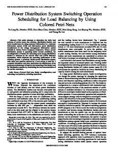
Figure 1 Suboptimal initial state

4.1 Suboptimal initial solution In this initial configuration, the switches 24, 34-52, 68 and 72 are closed, while the switches 1-23, 25-33, 53 and 69-71 are opened. Power flow calculation shows that 1300

the system losses in this configuration are P = 0,18751 MW (Fig. 1). The existing suboptimal state is tested by using the simulated annealing algorithm to see whether it actually gives an optimal solution or not. Simulations are performed at first with high starting Technical Gazette 22, 5(2015), 1297-1303

M. Stojkov i dr.

Optimizacija uklopnog stanja u distribucijskom elektroenergetskom sustavu

temperature and then with low starting temperature in combination at first with slow cooling and then with fast cooling. 4.1.1 High initial temperature t0 = 1000 and slow cooling kc = 0,99 In this case, 1013 configurations are established, 2062 simulations are obtained, the total simulation time is 375 seconds, and it is clear to see that there are 37 configurations with better solutions than starting configuration. Network configuration with minimal losses has power losses P= 0,17171 MW (Fig. 2).

Figure 4 Variation of losses at low initial temperature and slow cooling

4.1.4 Low initial temperature t0 = 100 and fast cooling kc = 0,95 In this case, 161 configurations are established, 360 simulations are obtained, the total simulation time is 81 seconds, and it is clear to see that there are 2 configurations with better solutions than starting configuration. Network configuration with minimal losses has power losses P = 0,18130 MW (Fig. 5).

Figure 2 Variation of losses at high initial temperature and slow cooling

4.1.2 High initial temperature t0 = 1000 and fast cooling kc = 0,95 In this case, 209 configurations are established, 405 simulations are obtained, the total simulation time is 90 seconds, and it is clear that there is 1 configuration with better solutions than starting configuration. Distribution network configuration with minimal losses has power losses P = 0,18376 MW (Fig. 3).

Figure 5 Variation of losses at low initial temperature and fast cooling

4.2 Randomly selected initial solution In this initial solution switches 2, 3, 5, 6, 9, 13, 15, 22, 25, 28, 29, 32, 33, 36, 38-46, 49-51, 53-55, 57-59, 61, 66, 67 and 72 are closed, while the switches 1, 4, 7, 8, 1012, 14, 16-21, 23, 24, 26, 27, 30, 31, 34, 35, 37, 47, 48, 52, 56, 60, 62-65 and 68-71 are opened. Power flow calculation shows that the power system losses in this configuration are P = 10,1874 MW (Fig. 6). The application of simulated annealing algorithm attempts to check if it is possible to get an optimal configuration like in the previous case. Figure 3 Variation of losses at high initial temperature and fast cooling

4.1.3 Low initial temperature t0 = 100 and slow cooling kc = 0,99 In this case, 779 configurations are established, 1833 simulations are obtained, the total simulation time is 297 seconds, and there are 18 configurations with better solutions than starting configuration. Distribution power network configuration with minimal losses has power losses P = 0,17171 MW (Fig. 4).

Tehnički vjesnik 22, 5(2015), 1297-1303

4.2.1 High initial temperature t0 = 1000 and slow cooling kc = 0,99 In this case, 990 configurations are established, 2062 simulations are obtained, the total simulation time is 381 seconds, and it is easy to see that applied simulated annealing technique gives an optimal configuration with minimal losses of P = 0,17171 MW (Fig. 7).

1301

Optimization of switching conditions in distribution power subsystem

M. Stojkov et al.

Figure 6 Randomly selected initial solution

Figure 7 Variation of losses at high initial temperature and slow cooling

Figure 9 Variation of losses at low initial temperature and slow cooling

4.2.3 Low initial temperature t0 = 100 and slow cooling kc = 0,99 In this case, 779 configurations are established, 1833 simulations are obtained, the total simulation time is 336 seconds, and applied simulated annealing method results in an optimal configuration of distribution network with minimal losses of P = 0,17171 MW (Fig. 9). 4.2.4 Low initial temperature t0 = 100 and fast cooling kc = 0,95 Figure 8 Variation of losses at high initial temperature and fast cooling

4.2.2 High initial temperature t0 = 1000 and fast cooling kc = 0,95 In this case, 197 configurations are established, 405 simulations are obtained, the total simulation time is 87 seconds, and applied simulated annealing optimization process gives an optimal configuration with minimal losses of P = 0,19314 MW (Fig. 8). 1302

In this case, 182 configurations are established, 360 simulations are obtained, the total simulation time is 79 seconds, and it is easy to see that applied simulated annealing optimization procedure gives an optimal configuration with minimal losses of P = 0,17832 MW (Fig. 10).

Technical Gazette 22, 5(2015), 1297-1303

M. Stojkov i dr.

Figure 10 Variation of losses at low initial temperature and fast cooling

5

Conclusion

The common characteristic of all generated simulations on this distribution subsystem is that the same optimal solution is obtained regardless of the initial solution being suboptimal or randomly selected. A slightly different solution is obtained with fast cooling and lower initial temperature. Therefore, it is always better to choose slower cooling with higher initial value of temperature, especially when it comes to the systems with much larger number of buses and switches. If we want to find an optimal solution as soon as possible, the starting temperature can be reduced, and the calculation will be accelerated, but it is related only to the systems with relatively small number of buses and switches. The advantage of slow cooling during the simulation performance is that the point of optimal solution is achieved more often. Therefore, the probability of getting the optimal solution is significantly higher. On the other hand, excessive acceleration of the cooling process leads to the point of reaching no optimal solution at all. From the point of finding an optimal solution, it is very important that this solution will meet certain established constraints in addition to minimizing the objective function. In the presented examples, the optimal configurations with minimal losses are found, and constraints at voltage levels in all buses are met and established. Regarding the implementation, this algorithm can be a useful tool for experienced engineers, especially for the fast finding of optimal configuration of the network in a case of sudden power outages of certain parts of the network or changes of network topology. The algorithm offers a range of optimal solutions and an experienced engineer can choose the one which is the most suitable for the application. 6

Optimizacija uklopnog stanja u distribucijskom elektroenergetskom sustavu

[5] Matos, M. A.; Melo, P. Multiobjective Reconfiguration for Loss Reduction and Service Restoration Using Simulated Annealing. // IEEE Power Tech ’99 Conference / Budapest, Hungary, 1999. [6] Matpower, A Matlab Power System Simulation Package. Version 3.0.0, 2005. [7] Zimmerman, R. D. Network Reconfiguration for Loss Reduction in Three-Phase Power Distribution Systems. MD partial fulfilment, Cornell University, May 1992. [8] Klaić, Z.; Šljivac, D.; Baus, Z. Probability Density Functions of Voltage Sags Measured Indices. // Journal of Electrical Engineering. 62, 6(2011), pp. 335-341. DOI: 10.2478/v10187-011-0053-8 [9] Klaić, Z.; Nikolovski, S.; Kraus, Z. Voltage variation performance indices in distribution network. // Tehnicki vjesnik-Technical Gazette. 18, 4(2011), pp. 547-551. [10] Kirkpatrick, S.; Gelatt C. D.; Yecchi, M. P. Optimization by Simulated Annealing. // Science, New Series. 220, 4598 (1983), pp. 671-680. DOI: 10.1126/science.220.4598.671 [11] Jeon, Y. J.; Kim, J. C.; Kim, J. O.; Shin, J. R.; Lee, K. Y. An Efficient Simulated Annealing Algorithm for Network Reconfiguration in Large-Scale Distribution Systems. // IEEE Trans. on Power Delivery. 17, 4(2002), pp. 10701078. DOI: 10.1109/TPWRD.2002.803823 Authors’ addresses Marinko Stojkov, PhD, Full Professor Josip Juraj Strossmayer University of Osijek Mechanical Engineering Faculty in Slavonski Brod Trg Ivane Brlić-Mažuranić 2 HR-35000 Slavonski Brod, Croatia E-mail: [email protected] Amir Softić, M.Sc. JP EP BiH Podružnica ED Tuzla Rudarska 38 BA-75000 Tuzla, Bosnia and Herzegovina E-mail: [email protected] MirzaAtić, PhD Gealan d.o.o. Maka Dizdara B-8 BA-75000 Tuzla, Bosnia and Herzegovina E-mail: [email protected]

References

[1] Abramson, D.; Randall, M. A Simulated Annealing Code for General Integer Linear Programs. Department of digital systems, Monash University, May 9, 1997. [2] Chang, H. C.; Kuo, C. C. Network Reconfiguration in Distribution Systems Using Simulated Annealing. National Taiwan inst. technology, 1994. [3] Chiang, H. D.; Jean-Jumeau R. Optimal Network Reconfigurations in Distribution Systems: Part 1: A New Formulation and a Solution Methodology. // IEEE. 5, (1990), pp. 1902-1909. [4] Rudnick, H.; Harnisch, I.; Sanhueza, R. Reconfiguration of Electric Distribution Systems. // Revista Facultad de Ingenieria, UTA (CHILE). 4, (1997), pp. 41-48. Tehnički vjesnik 22, 5(2015), 1297-1303

1303