New technological trends lead to the increasing use of network technologies in automation. Especially the. Ethernet with TCP/IP and wireless networks find grow ...
Optimizing Quality of Control in Networked Automation Systems using Probabilistic Models Jürgen Greifeneder and Georg Frey University of Kaiserslautern Erwin-Schrödinger-Str. 12 67663 Kaiserslautern, Germany {greifeneder,frey}@eit.uni-kl.de work. The two problems cannot be treated separately since for several applications a late package may have the same effect as a lost package. The scope of this paper is to demonstrate how Probabilistic Model Checking (PMC) can be used to improve quality, i.e. increase production accuracy, reduce rejected samples or decrease production times in a process controlled by a NAS. Clearly, in a system containing sensors and actuators connected via a network to a programmable logic controller (PLC), the accuracy of any given control action will depend on the delay occurring between a signal change at a sensor and the corresponding reaction at an actuator. This will be discussed in more detail within the case study in section 6. NAS are built of two types of components. First, there are those which might be shared by different users such as e.g. sensors, actuators, or switches; they induce waiting times. Second, there are cyclic processes which can be found e.g. in PLCs polling algorithms. Together, they form a behavior which contains time, stochastic distributions and probabilistic choice. Within this work, the modeling of these kinds of systems relies on Probabilistic Timed Automata (PTA, [1]) as discussed in more detail in section 3. The resulting automata are input to PMC, a formal technique for the analysis of systems described by PTA (cf. section 4). Section 7 concludes the paper and gives an outlook on further work.
Abstract New technological trends lead to the increasing use of network technologies in automation. Especially the Ethernet with TCP/IP and wireless networks find growing acceptance. The resulting networked automation systems (NAS) display properties such as stochastic delays and information loss, which are not known in classical automation structures. When control quality is to be assessed, these properties have to be determined. In this paper, the determination is achieved in a modeling approach based on Probabilistic Timed Automata (PTA). The derived models allow the analysis of delays using Probabilistic Model Checking (PMC). A case study will illustrate how the results of the analysis can be applied to increase the product quality in a manufacturing system controlled by an NAS.
1. Introductory Overview The rapid development of Ethernet or TCP/IP based technologies („internet technologies“) results in a collapse of prices for the corresponding hard- and software. For this reason developers and users of automation systems are replacing their domain-specific network technologies by Ethernet with TCP/IP. The new systems which result from the fusion of control systems (in terms of automation) and network technologies are called Networked Automation Systems (NAS). The general usability of Ethernet allows its adoption in different areas; it also offers the possible use of thus enabled additional functionalities, which lead to an increased and not previously predictable data flow. This additional dataflow may cause delays not present in classical structures. Furthermore, the use of wireless networks (WLAN, Zigbee) in NAS is rising, again due to the reduced cost of these technologies. Wireless networks, however, induce a potential risk of data loss during transmission. Hence, in the field of Networked Automation Systems, there are two critical points: firstly, the induced delay times, which can be described by a stochastic distribution rather than one constant value, and secondly, the possibility that information might get lost in the net-
1-4244-0681-1/06/$20.00 '2006 IEEE
2. Motivation Classical control theory deals with models containing an algorithm-based model for the controller and a model for the process derived either from physics or from measured data. The two models are connected to a closed-loop structure (cf. Fig. 1). Controller
Algorithm-based model
Process
Models derived fro m physics
Fig. 1. Closed-loop structure of controller and process in classical control and corresponding modeling approaches.
372
From there, the classical distributed control modeling was derived as illustrated in Fig. 2. Yet, there is still a number of controllers responsible (only) for their part of the process. In some implementations, there is a supervisor (algorithm-based modeling), in others, only some kind of information flows between the controllers. In special structures, completely independent controllers (only coupled by shared information on the process) can also possibly be used.
Chains (CTMC). As for CTMCs the probability of making a transition to a particular state must depend on the current state only, and it must be independent of the time elapsed since the entry into this state, there is only the exponential distribution which satisfies both of these conditions. Consequently, CTMCs are fine for modeling chemical reactors or other physical system in the continuous time domain. For NAS, this approach is not appropriate as it is not possible to use hard time guards. In this research domain, there are two other possibilities to deal with time.
Supervisor
Supervisor
C1
C2
C1
Cn
Cm
…
Controller Hardware
Middle layer
Network
P1
P2
Pn
I/O P1
Fig. 2. Classical distributed control model with controllers Ci and interconnected processes Pi.
I/O P2
Algorithm-based
Controller Hardware
…
I/O Pn
Physical-based
Fig. 3. Networked Automation System model with controllers Ci, processes Pi, corresponding Network-Interfaces (I/Ocards) and the network itself.
Now, this changes fundamentally in PLC-based distributed control approaches, where several sensors and actuators are communicating with different PLCs (cf. Fig. 3). In addition to possible waiting times induced by several users (i.e. control processes) sharing some common devices, the cyclic behavior of some components (e.g. PLCs) have to be considered as well as the behavior of the network and its components (“middle layer”). As all these effects induce delay times, it has to be checked whether they actually lead to system failures. Failures are defined as breakdowns of the system or its parts due to information arriving too late or not at all. Furthermore, there is an important influence on the product quality to be considered; therefore, the necessity to analyze the sequels of local dysfunctionalities, the occurrence of delay times and the dependence of the product quality on the entire system’s behavior arises. Since delay times have hitherto been discussed (e.g. [2]), this paper focuses on the projection of occurring delay times onto the (physical) manufacturing process. Unfortunately, classical analytical methods (e.g. worst case analysis) lead to infeasible demands on the automation system. Hence, rather colloquial expression the properties to be guaranteed are formulated using probabilistic bounds. Therefore, a modeling approach which can deal with time, stochastic distributions and probabilistic choice is used.
The first one (e.g. [4]) does not use time to satisfy a firing condition, but only for documentation and the relation (smaller, larger …) based decision which of several possibly activated transitions will be chosen. This again is not appropriate for NAS. The second approach (e.g. [3]) is more general, but needs the construction of a finite-state quotient representation prior to an analysis of the models (e.g. digital clocks or region graphs). Due to limitations in computational power, this second semantic is not applicable without a drastic reduction of the state space. Moreover, the deployed PMC-software (PRISM, [5]) does only support integer and Boolean variables. Therefore, the time domain is reduced to a finite set of steps within this work. Hence, the resulting automaton becomes congruent with the previously mentioned works of e.g. [4], as the firing condition becomes triggered by time and adjudicated by the non-time conditions. The analysis of a timed system using discrete time introduces certain artifacts, such as the trouble of finding an appropriate time step and a set of initial states which would at least be able to cope with constant time drifts among non-synchronized subsystems (cf. [6]). Time can be understood as a global state variable, implemented as a synchronized tick and local clocks. Finding an appropriate time step means choosing some fixed quantum a priori which limits the accuracy with which the system can be modeled (however: by using a time step which is shorter than necessary to exactly model the fastest system change, the size of the model has the tendency to increase exponentially). The time delay between two events is measured by counting the number of ticks between them. Consequently, it is impossible to state pre-
3. Modeling Approach Probabilistic timed automata are automata extended by clocks – leading to timed automata (TA, [3]) – and probabilistic choice. Dealing with times means dealing with real valued variables. This would be suitable throughout PMC by using Continuous Time Markov
373
cisely certain about delays. On the other hand, it involves the opportunity to eliminate the non-deterministic decisions by reducing the time-space to a discrete set of steps (respectively reducing the state space drastically by ignoring all possible combinations of occurrence within a really short period of time). From there onwards, it claims that the maximum length of a time step must be shorter than the time passing in between two consecutive significant events (where a significant event is an event which has an influence on other processes in the system). Again: as all significant choices are made synchronously now, the model will not represent the exact occurrence of an event, but only the fact that it occurred within the last time step. Yet, some systems will not allow the determination of the ideal length of such a time step in the way that each participating system will perform exactly one step in between two events. Additionally, the gradient of accuracy loss must be proven to be significantly smaller than the acuity of the result.
erties such as reliability, availability, safety, fault tolerance, robustness, and security. The investigation of the meaning of ‘dependability’ leads to the conclusion that dependability is a multi-attribute property, defined and measured by a set of different indicators; usually different stakeholders possess different definitions and requirements for dependability. 5.2. Quality of Service Dealing with networks, Quality of Service is mostly defined as a function of measurable parameters like packet loss, bandwidth, transmission- and delay times. It is linked to the specific needs of data transmission. A system analysis can thus reduce every network to a generic quality formula, whose value can be compared, optimized and so on. 5.3. Quality of Control The effectiveness of classical feedback controllers could be measured in terms of quality of control. This quality-factor (q-factor) is defined by a quadratic formula which uses values such as stability margin, convergence time, or overshot. This is possible because feedback control results in the generic problem of adjusting the controlled variables according to some reference and levering the disturbances. The problem becomes more complicated if the control loop is not built of a fixed wire any more, but fixed up by a TCP/IP based transmission. These so called network control systems (NCS) are current subject to several projects. While classical control problems can be expressed in generalized orders such as “adjust the control value” or “compensate the disturbance”, this is no longer possible for controlling devices in discrete systems. The properties in discrete systems can not be abstracted to generic formulas. Since, properties depending on the control specification such as “stop at the block”, “run five seconds” occur. This leads to the question if there can be a definition of quality of control in this kind of (manufacturing) context. Since the problem itself could not be generalized, the answer is no. However, it is possible to delineate the problem on a set of pre-defined templates, describing a generic approach. From these templates, a set of quality of service parameters should be derivable.
4. Probabilistic Model Checking In model checking [4], a model of the system is built upon some formal description. In addition, properties to be checked are formalized through the use of some kind of formal logic. These two descriptions are input to a model checking algorithm which checks whether the properties hold on the system. The problems which occur when this approach is extended to PMC are discussed in [2]. PMC uses an extension of Computation Tree Logic (CTL) called PCTL (Probabilistic Computation Tree Logic, [7]) to specify properties over systems described by Markov models. Typically, these properties are composed of atomic propositions or predicates over the variables in the model. Strictly speaking, it is distinguished between state and path constructs. PCTL formulae evaluate to a Boolean value; however, it is often useful to know the actual probability rather than just check whether the probability is above or below a given bound. Therefore, several implementations of PMC facilitate this functionality, which is used within this work. If PMC is used to analyze NAS, several advantages as well as disadvantages have to be considered. The advantages include that PMC covers for sure all possible evolutions of a system instead of only a subset as in simulation and testing procedures. The disadvantages are best described by the price to be paid given certain modeling abstractions, assumptions, and computational limits.
Definition: Quality of Control (QoC) in discrete event control systems (DECS) is defined as a performance vector. This measure of quality describes a quality quantity for the degree of attainment (mostly verbally) of predefined properties. Thereby, problem specific control properties are meant, i.e. these properties are functionally linked with the specific control task respectively the requirements of the specific plant. The degree of attainments’ description is realized on the basis of a realvalued vector with components residing in the interval ([0..1]).
5. Types of Quality 5.1. Dependability Dependability is defined by IFIP WG-10.4 as “The trustworthiness of a computing system which allows reliance to be justifiably placed on the service it delivers” [http://www.dependability.org]. For software, there is no dependability definition universally accepted and employed. Dependability is often regarded as a set of prop-
374
This QoC-vector in the most general case is determined by the definition of a set of quality characteristics (e.g. the relative number of delayed packages, medium values, distributions) and its multiplication with a weighting matrix. The elements of the resulting QoCvector then represent quality degrees for different subareas, e.g. reliability, accuracy, rejections, time quotient. It is possible to put these values in relation to one another, but other than in classical control theory it makes little sense to add them up. This is caused by a number of discontinuities, on the one hand, and the different meanings of the vector’s elements on the other hand. Finding an optimal solution is hence mostly finding a solution that accomplishes some given boundary conditions.
The influence of the NAS on the position-trajectory is shown in Fig. 5 for a single value-setting: xA=175, xB=5. While the upper curve shows a typical evolution for the case that the sensors’ signals act directly on the actuators, the lower curve shows the influence of the delay caused by the NAS on the positioning problem. First, both curves are identically until the first sensor is passed. Then, the system without NAS starts to decelerate, while the system with NAS still runs on high velocity until the signal is passed through the network (in this very example this takes 17 time steps). Afterwards, the system using NAS also decelerates down to vslow. 600 lu
500 400
6. Case Study
using NAS without NAS
300 200
6.1. System description The system under study (cf. Fig. 4) consists of a transport unit, which is driven by a speed controlled motor, a drilling unit and two inductive sensors. While the transport unit knows its speed, but is unable to determine its own position, the two inductive sensors – indicated with sA and sB – can only detect when a position (xA respectively xB) is reached.
tu
0 -100
PLC1IO write
cyclic requests
sA
xA
xB
30
40
50
Fig. 5: Illustration of a positioning process with direct sensor-actuator coupling in contrast to a NAS-system. When the object passes the sensor sA, this piece of information is passed through the network to the PLC-I/O card. From there, the value is written into the PLCs input buffer via a backplane-bus. Inside the PLC, the information is processed, this results in a new setting of an output variable used to slow down the motor from normal speed to a slow mode. The new output value is transferred via the PLC I/O-card and the network to the transport unit. The latter will execute the command as soon as the signal arrives. When the object passes the sensor at xB, the same procedure (as described above for sensor sA) will be accomplished, except that this time the transport unit will decelerate from the actual speed (which might still be larger than the slow mode speed, depending on when the ‘start decelerate for slow mode’ signal arrived) until it stops. After this state is reached, a stop signal is passed through the network to the PLC, and after being processed from there, the drilling command is issued. Obviously, by moving the positions of the sensors sA and sB, the accuracy of the drilling position can be optimized as well as the time needed for this processing task.
sB
Cycle time: 7 ts
20
-400
Outputs
PLC
10
-300
network
Cycle time:10 ts
0
-200
read
Execution
Inputs
100
0
v
Fig. 4: Architecture of the Networked Automation System used in the case study and schematic representation of the controlled process. The aim of the control is to achieve a given drilling position based on the sensors position xA and xB. The value to be optimized is the position where the drill puts the hole. The system is to be understood as NAS (this, of course, is a very small example, set up only to demonstrate the capacities). The two sensors are connected to an IO-card, which itself is connected to the network. The network is assumed to be wireless TCP/IPEthernet based. Package loss is not considered; for a discussion on that see e.g. [8]. The IO-access of the transport unit and the PLC-IO are also connected to the network. The PLC is connected to its IO-card via a shared memory (that is, incoming data will be available for the PLC as soon as it has arrived). The drilling process itself is not included in the model.
6.2. Abstractions and Assumptions The sensors are assumed to be exact within one length unit and the cyclic sensor-reading behavior is neglected. Both would add another delay distribution, which should be accounted for in a real system. However, those effects will not add a new phenomenon to this discussion (except another increase in calculation time). The net-
375
work itself is assumed to be TCP/IP-based wireless Ethernet containing an access point which acts as a router. Depending on other traffic conditions (e.g. signals from other sensors or to other actuators), the routing time varies in between one (90%) and two (10%) time steps. This corresponds to measurements at a lab system which finds most of the packages in between one and two milliseconds (i.e. one time step can be assumed to equal one millisecond). It is assumed that there is no other disturbance or delay within the network. For a discussion on consequences of failures in the network on the delay time see e.g. [2]. The PLC uses a cycle period of 7 time steps, while its I/O card cycle uses 10 time steps. The speed is assumed to be 24 length units per time step (lu/ts) in the normal mode and 4 lu/ts in the slow mode. The first deceleration is assumed to be 2 length units per time step square and the second one to be 4 lu/ts². These numbers are of an academic nature and designed to guarantee that all the state variables will represent an integer value after each time step. The definition for a length unit to be e.g. 0.01 mm with the given time step of 1ms results in reasonable values for speed and deceleration. The moment in which the object enters the system is of stochastic nature. Since the time step is fixed, the initial value of the position x has to inherit the stochastic character from the time: equally distributed over all possible initial values, i.e. with the initial (normal) velocity of 24 lu/ts the first value after entering the system ranges over 24 neighboring values. While this does not affect the medium end position, it has an effect on deviation and spread. It is more important for the result that PLC, PLC-I/O, motor and sensors are not synchronized, and therefore all possible permutations have to be considered by initial states (again, equally distributed). Furthermore, it is assumed that the relative time drift in between the modules is less than one time step over the total time period (i.e. that it is less than 1%). For the following discussion, these different initial states will not be considered, since they are merely important for the correctness of the results, but not for the way in which the new approach is built.
responding state explosion). Therefore, the network module was implemented in a simplified but generic way, i.e. only the packages are modeled, not the information carried by them. While this approach offers the opportunity to reuse this module, it necessitates that another module keeps track about the information. For each of the two sensors, a module with the following functionality was implemented: (1) register that the sensor got activated, (2) register when the corresponding package passed the network, (3) register when the PLC reaches its read-in state, (4) register when the PLC writes out the new value, (5) register when the PLC-I/O has sent it, (6) register the arrival of the package at the motor. Clearly, this module does not resemble an actual component of the system. However, it is really helpful since it allows the use of generic modules for the PLC as well as the PLC-I/O. These kinds of modules were named “signal tracking module” in [6]. count < Count Max-1
t count:=0
Inc(count)
t
t
count = Count Max-1
Fig. 6: Ring counter automaton: counting from zero to a maximum value and starting over again. Finally, there are three more modules. The first one recognizes the point of time when the velocity reaches zero and forces the automata transiting to a predefined termination state (the memory needed for this variable is less than the savings gained by a limitation of the terminal state space). The second module describes the transport unit position and activates the two sensors (cf. Fig. 7). The determination of the current value for x (x:=x+x‘·Δt+x“·(Δt)²) is abbreviated by Dm(x), while Δt equals one time step. t
Dm(x)
6.3. PMC model The PMC-model is composed of several modules. The PLC as well as the PLC-I/O is modeled as a ring-counter (counting from zero to a maximum value and starting over again) as discussed in [6], cf. Fig. 6. The variable t at the transitions symbolizes the synchronization over all modules. The network contains a waiting queue module (determining the current traffic and from there the “waiting time”) and a second module, passing the signals from the sensors to the PLC and from the PLC to the motor. Now, modeling the network with all detail would be like breaking a butterfly on a wheel (not mentioning the cor-
x0
Rx2&x‘>0
t
t t
x‘≤vslow &!Rx2
x‘=vslow x“=0 x‘≤vslow &!Rx2
x‘=0 x“=0
Note: This result could also be achieved by using the probability operator for all possible end positions and building the weighted sum afterwards.
t
true
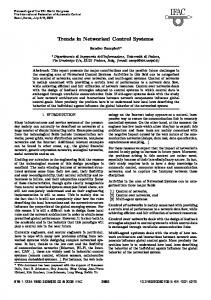
x‘≤0
t
6.6. Optimization and Results Fig. 15 shows the difference z between the medium end position (x) and the expected end position (xopt=1000 lu) as a function of the sensors’ positions xA and xB. Clearly, there are a number of combinations hitting the optimum. This calculation was done, using the R=? [F Stopped] operator as described earlier. The parallel lines at the top right of the figure shows that there is no solution possible for values of xA smaller than 627. In all other cases the trajectories gradient by passing the zero-line represents the sensitivity of the corresponding solution. Fig. 9 shows the percentage of values which lead to end positions outside given tolerance bounds (|z| >100 lu) as a function of xB for different values of xA., i.e. the difference from the expected end position is larger than 100 lu. Obviously, there are four local optima, namely for values of xA={663, 699, 735, 879}. A similar result can be found in Fig. 10 which shows the percentage of values which lead to variances larger than 141 lu.
t
Fig. 8: Automaton of the motor. 6.4. Limitations of the PMC-results Obviously, the discretization of the time axis leads to a small fuzziness in the results. By using a time discretization which would be 16 times faster this could be avoided on the one hand, but the state space would be blown. Therefore, determining the optimal time step length is not trivial and often enough subject to educated guesses. This problem might be solvable by using a discrete event approach which will be part of the future work. 6.5. PCTL-Formulae For an introduction to the use of PCTL, the reader is referred to the literature. In this work, the following PCTL-Formulae are used:
xA 0,4
probability (|x-xopt|>100)
P=? [true U (z>Lf)|(z20000) Probability ( variance > 141 lu )
Fig. 9: Probability of values outside xopt± 102. 0.3
xA 0.25
0.2
0.15
0.1
0.05
xA=663
xA>850
xA=735
0 0
100
200
300
400
xA=699
500
600
700
663 675 699 711 723 735 771 783 795 819 831 855 867 879
xB
Fig. 10: Percentage of value’s variance larger than 141 lu. In Fig. 11 there are also shown percentages of the value’s variances, this time using P=? [true U (z²Lf )
line) goes down smoothly, the one of the value pair {951,83} (dashed line) does not. As these are average values determined over all possible initial states, this means the following: In the case of the solid trajectory, the signal for decelerating to stop arrives in most cases before the slow speed is reached. This changes for the trajectory of {951,83}. Here the slow speed is run for some time. Hence it is not run by all evolutions at the same time and therefore the trajectory shapes as illustrated. From Fig. 13 further information can be derived: While in the case of {699,470} the longest run is determined to be 56, it is for sure larger than 120 in the second case.
Lf
0.8
Lf=25 0.5
Lf=50 0.4
Lf=75 0.3
Lf=100 0.2
Lf=125
0.1
xA
0
600
650
700
750
800
850
900
950
Fig. 11: Percentage of value's variance larger than a given bound (parameter Lf) for value pairs (xA, xB) derived from Fig. 15.
velocity
This together gives the impression, that xA should be chosen larger than 879. However, there is a price to be paid for it, namely the time needed by the transport unit to do the last 1000 length units as illustrated in Fig. 12: The earlier the deceleration is started, the longer the time to reach the selected end position. Finally a quality vector can be derived, containing the average end position, the deviation, the variance and the time. Table I shows this for those value pairs derived of Fig. 15.
20
xA
10
5
vslow 0
120
0
20
40
60
80
100
120
time
Fig. 13: Velocity trajectories for two selected value pairs: {699,470} – solid line – and {951,83} – dashed line
100
80
time
699 951
15
60
Fig. 14 gives the distribution of drilling positions (each point equals the probability that the deviation will be between this point and 1 lu further) for the above selected value pairs. While the 699-graph is flat, representing a wide spread range of final values, the 951, is much finer, representing a small range of end positions.
40
20
0 600
xA 650
700
750
800
850
900
950
Fig. 12: Time necessary to pass the last 1000 length units as a function of the value pairs derived from Fig. 15.
0.025
Table I: Quality vector for selected sensors’ positions xA
xB
Δx
Dev
var
time
663
542
0.157
10.2%
1.81‰
48.2
699
470
-0.088
6.98%
0.21‰
49.0
735
336
-0.031
16.1%
12.2‰
50.6
879
91
-0.300
0.006%
0
77.3
891
88
0.371
0
0
80.0
951
83
-0.370
0
0
92.5
0.02
0.015 699 951
xA
0.01
0.005
0 -120
The main difference in the results between the small values and the large values of xB is due to a different (average) velocity trajectory as demonstrated in Fig. 13. While the trajectory of the value pair {699,470} (solid
-70
-20
30
80
130
Fig. 14: Distribution of deviations from the optimal final position for two selected value pairs: {699,470} – solid line – and {951,83} – dashed line
378
z
was demonstrated how Probabilistic Model Checking (PMC) can be used to optimize the product quality in a NAS drilling positioning example. The next step in the presented work will be to transform the models from a constant time step approach to a discrete event approach, minimizing the number of steps in the model and thus (hopefully) reducing the memory and calculation time requirements. In this track, the transition to dense time and dense variables (the latter representing physical values) will be discussed also.
6.7. Modell sensitivity The sensitivity of the result in accordance to the NASstructure itself should be discussed: It is assumed that, due to higher network traffic, the time for a package to be sent increases from 1-2 time steps towards 1-5 time steps. Table II shows the resulting values as before in Table I. Table II: Quality vector for selected sensors’ positions, changed parameters xA
xB
Δx
Dev
var
Time
663
542
15.42
11.98%
11.9‰
48.93
699
470
16.25
9.56%
4.17‰
49.76
735
336
22.89
16.49%
31.77‰
52.0
879
91
6.00
0.19%
0
74.9
891
88
5.54
7.19%
0
77.3
951
83
2.95
0
0
89.2
References [1] [2] [3] [4] [5]
Obviously, the average end position get’s moved towards higher values. However, it also means an increased variance (not explicetely shown in Table II) which reduces the overall quality. If the cycle times of the PLC or the attached I/O-card are changed, a new optimization will be necessary, which will lead towards similar results.
[6]
[7]
7. Conclusions and Outlook
[8]
In this paper, a definition of quality in Networked Automation Systems (NAS) was presented. Together with a special modeling approach developed for NAS, it
R. Alur, C. Courcoubetis, and D. Dill, “Model-checking for probabilistic real-time systems”, in ICALP’91, LNCS, Vol. 510, Springer 1999, pp. 1–100. J. Greifeneder, and G. Frey, “Probabilistic delay time analysis in networked automation systems”, in 2005 IEEE ETFA Conf., Vol. 1, pp. 1065–1068. R. Alur and D. Dill. “A theory of timed automaton”. Theoretical Computer Science, 126(2): 183-235, 1994. B. Bérard, B., Bidiot, M., Finkel, A. Laroussinie, F. Petit, A., Petrucci, and L. Schnoebelen, “Systems and software verification, model-checking techniques and tools”, Springer, Ph. 2001. M. Kwiatkowska, G. Norman, and D. Parker. „PRISM: Probabilistic symbolic model checker”. In Proc. TOOLS’02, LNCS, vol. 2324, Springer, 2002, pp. 200–204. J. Greifeneder and G. Frey. “Determination of Delay Times in Failure Afflicted Networked Automation Systems using Probabilistic Model Checking”. Proceedings of 6th IEEE International Workshop on Factory Communication Systems (WFCS), Torino 2006, Italy, pp. 263–272. H. Hansson, and B. Jonsson, “A logic for reasoning about time and reliability”, in Formal Aspects of Comp. 6, no. 5, 1994. pp. 512–535. J. Greifeneder and G. Frey, “Dependability analysis of networked automation systems by probabilistic delay time analysis”, Proceedings of the IFAC Symposium on Information Control Problems in Manufacturing (incom), St. Etienne 2006, France, Vol. 1, pp. 269–274.
200
xA 519 531 543 555 567 579
100
591 603 615
final position z
627 639 651 663
xB
0
675 687 699
0
100
200
300
400
500
600
700
711 723 735 747 759 771 783
-100
795 807 819 831 843 855 867 879
-200
Fig. 15: Average drilling position as a function of the sensors' positions xA, xB. The intersection points created by the trajectories and the abscissa represent possible solutions of the optimization problem.
379