May 24, 2013 - fields of research, ranging from percolation in statistical physics [1], the .... i {ci1[ti = 0] â ri1[ti < â]} where ci is the cost of selecting vertex i as a ...
Optimizing spread dynamics on graphs by message passing F. Altarelli,1, 2 A. Braunstein,1, 3, 2 L. Dall’Asta,1, 2 and R. Zecchina1, 3, 2 1
arXiv:1203.1426v2 [cond-mat.dis-nn] 24 May 2013
DISAT and Center for Computational Sciences, Politecnico di Torino, Corso Duca degli Abruzzi 24, 10129 Torino, Italy 2 Collegio Carlo Alberto, Via Real Collegio 30, 10024 Moncalieri, Italy 3 Human Genetics Foundation, Via Nizza 52, 10126 Torino, Italy
Cascade processes are responsible for many important phenomena in natural and social sciences. Simple models of irreversible dynamics on graphs, in which nodes activate depending on the state of their neighbors, have been succesfully applied to describe cascades in a large variety of contexts. Over the last decades, many efforts have been devoted to understand the typical behaviour of the cascades arising from initial conditions extracted at random from some given ensemble. However, the problem of optimizing the trajectory of the system, i.e. of identifying appropriate initial conditions to maximize (or minimize) the final number of active nodes, is still considered to be practically intractable, with the only exception of models that satisfy a sort of diminishing returns property called submodularity. Submodular models can be approximately solved by means of greedy strategies, but by definition they lack cooperative characteristics which are fundamental in many real systems. Here we introduce an efficient algorithm based on statistical physics for the optimization of trajectories in cascade processes on graphs. We show that for a wide class of irreversible dynamics, even in the absence of submodularity, the spread optimization problem can be solved efficiently on large networks. Analytic and algorithmic results on random graphs are complemented by the solution of the spread maximization problem on a real-world network (the Epinions consumer reviews network).
Contents
I. Introduction II. The Spread Optimization Problem A. Related Work B. The Linear Threshold model
2 2 2 3
III. The Message-Passing Approach A. Mapping on a Constraint-Satisfaction Problem B. Derivation of the Belief-Propagation equations C. Derivation of the Max-Sum equations D. Efficient computation of the MS updates E. Simplification of the MS messages F. Time complexity of the updates G. Convergence and reinforcement
3 3 4 5 6 7 8 8
IV. Results A. Validation of the algorithm on computer-generated graphs B. Spread maximization in a social network C. Role of Submodularity
8 8 10 11
V. Summary and conclusions Acknowledgments
12 12
A. Efficient update equations for BP
12
B. Alternative algorithms 1. Linear Programming Algorithm 2. Greedy Algorithms 3. Simulated Annealing
14 14 14 14
2 C. Simulated Annealing on the Epinions graph References
15 15
I.
INTRODUCTION
Recent progress in the knowledge of the structure and dynamics of complex natural and technological systems has led to new challenges on the development of algorithmic methods to control and optimize their behavior. This is particularly difficult for large-scale biological or technological systems, because the intrinsic complexity of the control problem is magnified by the huge number of degrees of freedom and disordered interaction patterns. Even simple to state questions in this field can lead to algorithmic problems that are computationally hard to solve. For instance, the problem of identifying a set of initial conditions which can drive a system to a given state at some later time is in most cases computationally intractable, even for simple irreversible dynamical processes. This is however a very relevant problem because irreversible spreading processes on networks have been studied since long time in several fields of research, ranging from percolation in statistical physics [1], the spread of innovations and viral marketing [2– 5], epidemic outbreaks and cascade failures [6, 7], avalanches of spiking neurons [8], and financial distress propagation in the interbank lending networks [9–12]. In typical applications, the nodes of a network can be in one of two states (e.g. “active” and “inactive”), according to some dynamical rule which depends on the states of neighboring nodes. Computer simulations and mean-field methods have shed light on the relation between the average behavior of macroscopic quantities of interest, such as the concentration of active nodes, and the topological properties of the underlying network (e.g. degree distribution, diameter, clustering coefficient), but they provide no effective instrument to optimally control these dynamical processes [13]. Overcoming this limitation is crucial for real-world applications, for instance in the design of viral marketing campaigns, whose goal is that of targeting a set of individuals that gives rise to a coordinated propagation of the advertisement throughout a social network achieving the maximum spread at the minimum cost. A similar optimization process can be applied to identify which sets of nodes are most sensitive for the propagation of failures in power grids or which sets of banks are “too contagious to fail”, providing a tool to assess and prevent systemic risk in large complex systems. It is known that simple heuristic seeding strategies, such as topology-based ones, can be used to improve the spread of the process [14] as compared to random seeding. In order to attack this optimization problem in a systematic way, one should be able to analyze the large deviations properties of the dynamical process, i.e. exponentially rare dynamical trajectories corresponding to macroscopic behaviors that considerably deviate from the average one. At the ensemble level, this was recently put forward in [15]. In the present work we consider the optimization aspects, developing a new algorithm based on statistical physics that can be applied to efficiently solve this type of spread optimization problems on large graphs. As a case study, we provide a validation and a comparative analysis of the maximization of the spread of influence in a large scale social network (the “Epinions” network). Our results show that the performance of the optimization depends on the nature of the collective dynamics and, in particular, on the presence of cooperative effects. The paper is organized as follows. In Section II we introduce the spread optimization problem, focusing on a particular model of irreversible propagations on graphs, and we discuss the related literature. Section III is devoted to the derivation of the message-passing approach to the spread optimization problem, while the validation of the method on computer-generated graphs and the results obtained on the real-world network are presented in Section IV.
II.
THE SPREAD OPTIMIZATION PROBLEM A.
Related Work
The problem of maximizing the spread of a diffusion process on a graph was first proposed by Domingos and Richardson [16] in the context of viral marketing on social networks. The problem can be summarized as follows: given a social network structure and a diffusion dynamics (i.e. how the individuals influence each other), find the smallest (or less costly) set of influential nodes such that by introducing them with a new technology/product, the spread of the technology/product will be maximized. Kempe et al. [17] gave a rigorous mathematical formulation to this optimization problem considering two representative diffusion models: the independent cascade (IC) model and the Linear Threshold (LT) model. They studied the problem in a stochastic setting, i.e. when the dynamics is based on randomized propagation, showing that for any fixed parameter k it is NP-hard to find the k-node set achieving the maximum expected spread of influence. They proposed a hill-climbing greedy algorithm, analogous to the greedy set
3 cover approximation algorithm [18], that is guaranteed to generate a solution with a final number of active nodes that is provably within a factor (1 − 1/e) of the optimal value for both diffusion models [17]. In the greedy algorithm, the nodes that generate the largest expected propagation are added one by one to the seed set. Because of the stochastic nature of the problem, the algorithm is computationally very expensive, because at each step of the process one has to resort to sampling techniques to compute the expected spread. Leskovec et al. [19] proposed a “lazy-forward” optimization approach in selecting new seeds that reduces considerably the number of influence spread evaluations, but it is still not scalable to large graphs. Chen et al. [20] proved that the problem of exactly computing the expected influence given a seed set in the two models is #P-hard and provided methods to improve the scalability of the greedy algorithm. For a more comprehensive review of techniques and results, see e.g. [21]. Real diffusion processes on networks are likely to be intrinsically stochastic, and information on the properties of the real dynamics might be obtained by surveys or data mining techniques [22]. Different forms of stochasticity seem to make great difference on the properties of the optimization problem. In fact, only a peculiar choice of the distributions of parameters (e.g. uniform thresholds on a given interval for the LT model [17]) makes possible the derivation of the approximation result and guarantees good performances of the greedy algorithm. On the other hand, the apparently simpler case represented by the deterministic LT model [2] was proven to be computationally hard even to approximate in the worst case[23]. This is due to the lack of a key property, known as submodularity [24], that is necessary to prove the approximation bound of Kempe et al. [17] and that will be discussed later.
B.
The Linear Threshold model
The deterministic Linear Threshold model was first proposed by Granovetter [2] as a stylized model of the adoption of innovation in a social group, motivated by the idea that an individual’s adoption behavior is highly correlated with the behavior of her contacts. The model assumes that the influence of individual j on individual i can be measured by a weight wji ∈ R+ , and that i’s decision on the adoption of an innovation only depends on whether or not the total influence of her peers that already adopted it exceeds some given personal threshold θi ∈ R+ . In a social network, represented by a directed graph G = (V, E), individuals are the nodes of the graph and they can directly influence only their neighbors. At each time step, a node i ∈ V can be in one of two possible states: xi = 0 called inactive and xi = 1 called active, that corresponds to the case in which i adopts the product. A vertex which is active at time t will remain active at all subsequent times, while a vertex which is inactive at time t can become active at time t + 1 if some threshold condition, depending on the state of its neighbors in G at time t, is satisfied. More precisely, given an initial set of nodes that are already active at time t = 0, the so-called seeds of the dynamics, the dynamical rule is as follows ( P t 1 if xti = 1 or t+1 j∈∂i wji xj ≥ θi , xi = (1) 0 otherwise , where ∂i is the set of the neighbors of i in G. Note that by interpreting empty sites as active nodes, the Bootstrap Percolation process from statistical physics [1] becomes a special case of the LT model.
III. A.
THE MESSAGE-PASSING APPROACH
Mapping on a Constraint-Satisfaction Problem
In the LT model, the trajectory {x0 , . . . , xT } (with xt = {xti , i ∈ V }) representing the time evolution of the system can be fully parametrized by a configuration t = {ti , i ∈ V }, where ti ∈ T = {0, 1, 2, . . . , T, ∞} is the activation time of node i (we conventionally set ti = ∞ if i does not activate within an arbitrarily defined stopping time T ) [34]. Given a set of seeds S = {i : ti = 0}, the solution of the dynamics is fully determined for i ∈ / S by a set of relations among the activation times of neighboring nodes, which we denote by ti = φi ({tj }) with j ∈ ∂i. In the LT model, the explicit form of the constraint between the activation times of neighboring nodes is then X ti = φi ({tj }) = min t ∈ T : wji 1[tj < t] ≥ θi (2) j∈∂i
where the indicator function 1[condition] is 1 if ‘condition’ is true and 0 otherwise. This constraint expresses the rule that the activation time of node i is the smallest time at which the sum of the weights of its active neighbors reaches
4
FIG. 1: Dual factor graph representation for the spread optimization problem
the threshold θi . Admissible dynamical trajectories do correspond to configurations of activation times t such that the binary function Ψi = 1[ti = 0] + 1 [ti = φi ({tj })] equals 1 for every node i. We then introduce an energy function E (t) to give different probabilistic weights to trajectories with different activation times, P[t] ∝ exp[−βE (t)]. The specific form of the energy P function will depend on the features of the trajectory that one wishes to select. In the most general form, E (t) = i Ei (ti ) where Ei (ti ) is the “cost” (if positive, or “revenue” if negative) incurred by activating vertex i at time ti . When β is large (compared to the inverse of the typical energy differences between trajectories), the distribution will be concentrated on those rare trajectories with an energy much smaller than the average, i.e. the large deviations of the distribution. When β → ∞, only the trajectory (or trajectories) with the minimum energy are selected. Notice that the value chosen for T will affect the “speed” of the propagation: a lower value of T will restrict the optimization to “faster” trajectories, at the (possible) expense of the value of the energy. Solving the Spread Maximization Problem (SMP) corresponds to selecting the trajectories that activate the largest number of nodes with the smallest number of seeds, or more precisely which minimize the energy function E (t) = P {c 1 [t i i = 0] − ri 1 [ti < ∞]} where ci is the cost of selecting vertex i as a seed, and ri is the revenue generated by i the activation of vertex i (independently of the activation time). We consider the values of {ci } and {ri } as part of the problem definition, together with the graph G, the weights {wij } and the thresholds {θi }. Trajectories with small energy will have a good trade-off between the total cost of the seeds and the total revenue of active nodes.
B.
Derivation of the Belief-Propagation equations
The representation of the dynamics as a high dimensional static constraint-satisfaction model over discrete variables (i.e. the activation times) makes it possible to develop efficient message-passing algorithms, inspired by the statistical physics of disordered systems [25], that can be used them find a solution to the SMP. Our starting point is the finite temperature version (β < ∞) of the spread optimization problem, in which a Belief-Propagation (BP) algorithm can be used to analyze the large deviations properties of the dynamics [15]. The Belief Propagation algorithm is a general technique to compute the marginals of locally factorized probability distributions under a correlation decay assumption [26]. A locally factorized distributionP for the variables t = {ti , i ∈ V } is a distribution which can be written in the form P (t) ∝ exp[−F (t)] with F (t) = a Fa (ta ) where each factor contains only a (generally small) subvector ta of t. The correlation decay assumption means that in a modified distribution in which the term Fa (ta ) is removed from the sum forming F (t), the variables in ta become uncorrelated (the name cavity method derives from the absence of this single term). The factor graph representing the distribution is the bipartite graph where one set of nodes is associated to the variables {ti }, the other set of nodes to the factors {Fa } of the distribution, and an edge (ia) is present whenever ti ∈ ta . When the factor graph is a tree, the correlation decay assumption is always exactly true. Otherwise a locally tree-like structure is usually sufficient for the decorrelation to be at least approximately verified. In the activation-times representation of the dynamics, the factor nodes {Fa } are associated with the dynamical constraints Ψi (ti , {tj }j∈∂i ) and with the energetic contributions Ei (ti ). Since nearby constraints for i and j share the two variables ti and tj , it follows that the factor graph contains short loops. In order to eliminate these systematic short loops, we employ a dual factor graph in which variable nodes representing the pair of times (ti , tj ) are associated to edges (i, j) ∈ E, while the factor nodes are associated to the vertices i of the original graph G and enforce the hard constraints Ψi corresponding as well as the contribution from i to the energy function. Figure 1 gives an illustrative example of such dual construction. The quantities that appear in the BP algorithm are called cavity marginals or equivalently beliefs, and they are associated to the (directed) edges of the factor graph. We call Hi` (ti , t` ), the marginal distribution for a variable
5 (ti , t` ) in the absence of the factor node F` . Under the correlation decay assumption, the cavity marginals obey the equations [15] X Y Hij (ti , tj ) ∝ e−βEi (ti ) Ψi (ti , {tk }k∈∂i ) Hki (tk , ti ). (3) {tk }k∈∂i\j
k∈∂i\j
These self-consistent equations are solved by iteration. In Appendix A we show how to compute these updates in a computationally efficient way not discussed in [15]. Q Once the fixed point values of the cavity marginals are known, the “full” marginal of ti can be computed as Pi (ti ) ∝ j∈∂i Hji (tj , ti ) and the marginal probability that neighboring nodes i and j activate at times ti and tj is given by Pij (ti , tj ) ∝ Hij (ti , tj )Hji (tj , ti ). In all equations the proportionality relation means that the expression has to be normalized. Equation (3) allows to access the statistics of atypical dynamical trajectories (e.g. entropies of trajectories or distribution of activation times). However it does not provide a direct method to explicitly find optimal configurations of seeds (in terms of energy). To this end, we have to take the zero-temperature limit (β → ∞) of the BP equations, and derive the so-called Max-Sum (MS) equations. C.
Derivation of the Max-Sum equations
Writing explicitly the constraints and the energetic terms, the BP equations (3) read X Y −βc i Hji (tj , 0) if ti = 0, e {t , j∈∂i\`} j∈∂i\` j Y X Hji (tj , ti ) if 0 < ti ≤ T , j∈∂i\` {t , j∈∂i\`} s.t: j P Hi` (ti , t` ) ∝ w 1[t ≤t −1]≥θi , Pk∈∂i ki k i wki 1[tk