Orthogonal and Non-Orthogonal Joint Blind Source Separation in the

20th European Signal Processing Conference (EUSIPCO 2012)

Bucharest, Romania, August 27 - 31, 2012

ORTHOGONAL AND NON-ORTHOGONAL JOINT BLIND SOURCE SEPARATION IN THE LEAST-SQUARES SENSE Marco Congedo, Ronald Phlypo, Jonas Chatel-Goldman Equipe ViBS (Vision and Brain Signal Processing), GIPSA-lab, CNRS, Grenoble University, France we suppose that each data set is multidimensional, such

ABSTRACT

as xm  t    xm   t  ,..., xm 1

We present two new algorithms for the orthogonal and nonorthogonal joint blind source separation (JBSS), a flexible framework that extends the well-known blind source separation to the case when multiple datasets are decomposed simultaneously. The algorithms minimize the total sum of squares of the off-diagonal terms by means of very simple gradient ascent iterations. Index Terms— Joint Blind Source Separation, Hyperscanning, Brain Coupling, Synchronization. 1. INTRODUCTION Blind Source Separation (BSS) is a well-known framework including Independent Component Analysis and other decomposition methods aiming at recovering source signals in MIMO systems [1]. BSS nowadays encompasses a wide range of engineering applications such as speech enhancement, image processing, geophysical data analysis, wireless communication and biomedical signal analysis. Generally speaking, BSS takes as input a multivariate linearly mixed signal received over N sensors and outputs a P≤N multivariate demixed signal. More recently the joint blind source separation (JBSS) approach has been proposed in biomedical imaging [2-5]. Whenever M datasets are available and a relation exists among the sources of the M sets, this approach exploits the joint statistics of the M datasets by solving the M BSS problems simultaneously rather than independently. Several algorithms for performing JBSS in the case of orthogonal mixing matrices have been proposed [2-5]. In this paper we extend previous work performed on BSS [5-7] and we describe a leastsquares gradient approach to JBSS allowing a simple solution for both the orthogonal and nonorthogonal case. 2. METHOD 2.1. Problem Statement Suppose we are given M datasets, with m=1,…,M. As usual,

© EURASIP, 2012 - ISSN 2076-1465

N

 t 

T

,

wherein

N

random

variables hereafter indexed by n=1,…,N, unfold over the discrete dimension t=1,…,T. Note that n and t may refer to, for instance, space and time, respectively, as it is the case for the human electroencephalogram (EEG), but this is not important for the sequel. Suppose further that K observations are available for each dataset, indexed by k=1,…,K, yielding KM groups of N variables, hereafter denoted compactly as xm,k  t  . To give just a few examples, in the second-order statistics framework the K observations may refer to K experimental conditions, to recordings in K different times (or trials), or to an expansion of the original data in K discrete frequencies or K time-frequency regions. We assume the following generative model for the data: xm,k  t   Am sm,k  t   ηm,k  t 

(1.1)

where AmℝNxP is a (t, k)-invariant full column rank mixing matrix, sm,k(t) ℝP, with P≤N, holds the source components over the t dimension and m,k(t) ℝN is spatially uncorrelated additive noise, assumed also uncorrelated with sm,k(t). Notice that the mixing matrix is specific to each dataset, but is the same for each dataset along the K observations. This model is an extension to multiple datasets of the typical model found in the BSS literature. It has been proposed already several times [2-5, 8]. It reduces to the very common model used in BSS xk  t   Ask  t   ηk  t  when only one dataset is available. In JBSS we require to find the M matrices BmℝNxP, m=1,…,M, yielding the source estimates sm,k  t   BmT xm,k  t  , where, under mild assumptions on the noise, the demixing matrices Bm estimate the Moore-Penrose pseudo-inverse of the mixing matrices up to a sign, scale and permutation indeterminacy, as in the BSS case. However in JBSS we require the permutation be the same for all M datasets, otherwise the analysis of the corresponding sources in the M datasets becomes difficult. This is, among others, a key advantage of the JBSS approach. Notice that for the sake of simplicity we suppose hereafter that N=P, this quantity being the same across datasets.

1885

  T 2  tot Bi |B     2tr  Qij , k Qij ,k   tr  Qii ,k   and k  j i 

2.2. The Joint Blind Source Separation (JBSS) In order to apply JBSS we extract K[M(M+1)/2] matrices of second-order statistics from the K observations of M multivariate datasets [2, 5, 8]. From Eq. (1.1) these matrices follow the theoretical model Cij ,k  Ai Λij ,k ATj  Nij ,k , with i,j=1,…,M,

(1.2)

where the ij,k matrices, the unknown source statistics, are supposed all diagonal, surely non-null if i=j (auto-statistics within datasets) and possibly non-null even for i≠j (crossstatistics between corresponding sources of the i and j datasets). The matrices Nij,k are unknown noise matrices holding additive measurement noise and sample estimation errors. In order to estimate the M demixing matrices we seek matrices making all K[M(M+1)/2] distinct products Qij ,k  BiT Cij ,k Bj

(1.3)

as diagonal as possible. This implies that the output (source) statistics within datasets are diagonalized (for i=j), as in the BSS framework. In addition, the output cross-statistics between datasets are also diagonalized, thus corresponding sources across datasets may be correlated. Notice that Cij,k=CTji,k, thus it suffices to consider K[M(M+1)/2] products instead of all KM 2 products. 2.3. Least-Squares Functional We want to find matrices BTm minimizing the sum of squares of the elements outside the diagonals of all Qij,k, that is

min

B1 ,..., BM

 off  B C T i

ij ,k

i , j ,k

Bj 

2 F

off Bi |B  2 off  Qij ,k  k



2 F

 off  Qii ,k  k

2 F

2

T i n

n

T ii ,k i  n 

b

  (1.7) 2

2.4. The Orthogonal Mixing Matrices Case In this case the exact estimation of Bi is equal to Ai up to permutation and scale indeterminacy, for all m=1,…,M and it is well known that the “total” function is invariant with respect to B. Thus we are left with the problem of maximizing iteratively the “diag” functional in (1.7), for i=1,…,M. Let us rewrite the objective function as 2 2    diag  diag  Qii ,k   , Bi |B    2 diag  Qij , k  F F k  j i j i  where the diag operator nullifies the off-diagonal elements of the matrix argument, and then as     2  tr  EnQij ,k En EnQ ji ,k En   j i  n  ,  diag Bi |B    k   tr EnQii ,k En EnQii ,k En    n









where matrix En is the elementary matrix filled with entry 1 at position (n,n) and 0 elsewhere. The above function is a matrix polynomial of second degree in Bi. The derivative is of first degree in Bi for the first trace and of third degree in Bi for the second trace. However, using the symmetry of matrices Cii,k, the gradient simplifies to   diag Bi |B Bi

Thus where

 4 Cij ,k Bj En En Q ji ,k En    j i n    . k  4Cii ,k Bi En En Qii ,k En   n  

  diag Bi |B Bi

 4  Mi 1 bi 1 ,..., Mi  N  bi  N   ,  





Mi  n    Cij ,k b j  n  bTj  n CijT,k . k

j

(1.8) (1.9)

, (1.4)

wherein we have used Eq. (1.3) and we have separated the partitions for i≠j (firt Frobenius norm) and the partition for i=j (second Frobenius norm). Equation (1.4) can also be written such as tot  diag diag off  tot (1.5) Bi |B   Bi |B Bi |B   Bi |B , where the “total” and “diagonal” parts are

    b  C

respectively. In Eq. (1.7), bi(n) is the nth column vector of Bi, with n=1,…,N and bTi(n) its transpose.

,

where the off operator nullifies the diagonal elements of the matrix argument. The overall strategy is to sequentially search for each matrix Bi, for i=1,…,M and iterate such sequential search until convergence. Let us denote with B the set of all demixing matrices. In the sequel, following [3], let us define the functional of interest for any given i=1,…,M as

j i

 T T  diag Bi |B    2 bi  n Cij , k b j  n  k  j i n

(1.6)

In words, the gradient of the N vectors of Bi should be taken as the eigenvectors of corresponding matrices Mi(n) associated with their largest eigenvalue, for all n=1,…,N. In order to update these vectors we limit ourselves to a single power iteration [6-7]. After updating all vectors of Bi we need to orthogonalize Bi so as to ensure that at each step Bi stays in the orthogonal group [5]. Therefore, we have the following simple updating rule:

1886

that is, the sum of matrices already found in (1.9). Setting the gradient to zero gives us a stationary point for our optimization, which for each Bi is given by MiBi=[Mi(1)bi(1),…,Mi(n)bi(n)]. This is a generalized eigenvalue-eigenvector problem, where each bi(n) is the eigenvector of Mi(n) in the metric of Mi. Again, limiting ourselves to one single power iteration per update step, this yields the simple updating rule:

  B   Mi 1 bi 1 ,..., Mi  N  bi  N   for all i=1,…,M do  i .  orthogonalize Bi The iterative algorithm is summarized here below:

Algorithm OJoB (Orthogonal Joint BSS) Initialize B1,…,BM as orthogonal matrices (e.g., identity) Repeat For i=1,…,M do Compute the N matrices Mi(n) using (1.9) For n=1,…,N do bi(n)←Mi(n) bi(n) Bi ← (BiTBi)-1/2Bi Until Convergence

 B  M 1  M b ,..., M b  i  i 1 i 1 i N  i N    i  For i=1,…,M do for n =1,...,N do .  1/2 T bi  n   bi  n  bi  n  Mi  n  bi  n  



Note that in practice the orthogonalization is computed faster as Bi←UVT, where UΓVT is the SVD of Bi [5]. 2.5. The Non-Orthogonal Mixing Matrices Case

In practice, we sought to avoid the computation of the matrix inverse, therefore we proceed more efficiently, albeit equivalently, in the following way : Algorithm NOJoB (Non-Orthogonal Joint BSS) Initialize B1,…,BM so as to satisfy constraint in (1.10) Repeat For i=1,…,M do Get the N matrices Mi(n) using (1.9) and their sum Mi Do Cholesky decomposition Mi=LLT. For n=1,…,N do Solve Lx=Mi(n)bi(n) for x and LTy=x for y bi(n)←y(yTMi(n) y)-1/2 Until Convergence

In this case the “total” function is not invariant to B, hence we need to explicitly minimize the “off” functional in (1.4). Furthermore we need to avoid the trivial solution BTm=0, for any m=1,…,M. Therefore, we minimize the “off” functional in (1.5)-(1.7) with a constraint (w.c.) on the norm of the column vectors of Bm, such as  diag tot , w.c. biTn  Mi n  bi n   1, n  1,..., N , (1.10) Bi |B

where matrices Mi(n) are given in (1.9). Note that this is an “intrinsic” constraint, as proposed first in [6-7]. We use the method of Lagrange multipliers to turn (1.10) into an unconstrained optimization problem. The method leads us to minimize    diag L  tot    2 tr  Qij ,k Q ji ,k   tr  Qij2,k   Bi |B k  j i 







 B j En2Q ji ,k En   4  n  Cii ,k Bi En2Qii ,k En  k  j i n n  where the Lagrangian multipliers δn are adjusted in order to satisfy the constraint. Using again the symmetry of the matrices Cii,k and exploiting the previous results in (1.8), the gradient of the Lagrangian reads

 4  C n



 diag L  tot Bi |B

Bi

or





ij , k

   Cij,k BjQij,k   4 Cii,k BiQii,k   BBi |B k 4 i  j i 

 diag L  tot Bi |B

diag

  4M B  4  M i

Bi

i



b ,..., Mi  N  bi  N   , 

i 1 i 1

where Mi    Cij ,k B j BTj CijT,k    Mi  n  , k

j

n



3. RESULTS In this section the behavior of the proposed algorithms is assessed by means of simulations. Input matrices Cij,k are generated according to the model in Eq.(1.2); matrices ij,k are generated as square diagonal matrices with each diagonal entry randomly distributed as a chi-squared with M degrees of freedom and divided by M; noise matrices Nij,k are symmetric and have entries randomly Gaussian distributed with zero mean and σ standard deviation (sd). The parameter σ controls the signal to noise ratio of the input matrices. Several different values of σ will be considered in the simulations. The mixing matrices Am, m=1,…,M, are generated as orthogonal or non-orthogonal. Orthogonal matrices are generated by first generating a matrix with entries randomly drawn from a Gaussian distribution with zero mean and sd=1 and then taking its left singular vector matrix. In this case the conditioning of the mixing matrices does not jeopardize the performance of the algorithms and we can evaluate their robustness with respect to noise. In order to generate non-orthogonal matrices, the matrices generated as above are perturbed by adding to each entry a number randomly drawn from a Gaussian distribution with zero mean and sd=1/2. In this case the mixing matrices have variable conditioning and we can

1887

evaluate the behavior of the algorithms with respect to the conditioning of the mixing matrices. The algorithms estimate the demixing matrices BT1,…,BTM, which should approximate the pseudo-inverse of actual mixing matrices A1,…,AM up to row scaling (including sign) and global permutation. Then, matrices Gm= BTmAm should approximate as much as possible a scaled permutation matrix [1]. For each estimated demixing matrix we consider the Amari-like performance index [1], which is computed as

where indexes x and y run over 1,…,N (rows and columns of matrices Gm), gmxy is the (x,y) entry of matrix Gm, and |.| denotes the absolute value of the argument. We define the composite performance as a function of the geometric mean of the performance indexes obtained over the M matrices, such as





4. CONCLUSION We have presented two new algorithms performing JBSS in a least-squares framework. Preliminary results encourage further investigation. Before NoJoB, only one nonorthogonal JBSS algorithm has been proposed [8].

m     g xy gm  y       x xy  1 2 N  N  1 , m    1 m m  y  max g xy  x  max g xy  x   y 

   log10 1  M  m 1   m  .

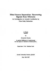
Figure 2 shows the performance of the NoJoB algorithm (yaxis) vs. the mixing matrices conditioning (1.12) with nonorthogonal mixing (input) matrices, N=P=3 and several combinations of M, K, and σ. Results show that the more noise there is in the system the more the conditioning affects the performance. Furthermore, the degradation is not mitigated by increasing K and only moderately mitigated by increasing M.

(1.11)

Values of π above 2 indicate a very good performance. Note that the composite performance defined this way is dominated by the worst performance over the M performances. The higher the value of the composite index (1.11), the higher the performance. Likewise, the composite conditioning with respect to matrix inverse of the mixing matrices is defined as

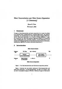
  log10   m max eig  Am  / min eig  Am   , (1.12) where maxeig and mineig are the largest and smallest eigenvalue of the argument, respectively. Figure 1 shows the performance (1.11) obtained by the OJoB and NoJoB algorithms with orthogonal mixing (input) matrices, N=P=3 sensors/sources and several combinations of M (number of datasets), K (number of observations), and σ (noise level). One hundred simulations have been performed for each algorithm and for each combination of M, K and σ. Each dot represent the intersection of the performance obtained in one simulation when the algorithm is initialized with identity matrices (x-axis), that is, possibly far from the optimal solution, and with the exact solutions (y-axis). Dots lying on the 45° line indicate that the algorithms have a stable attractor, despite the added noise. Dots lying above the 45° line indicate that the algorithm gets far from the exact solution. These results show that for both algorithms the degradation engendered by noise is mitigated by increasing either K or M. Also, when either M or K are much larger than N no divergence of the algorithms is noticed. Overall, NoJoB appears more stable than OJoB.

5. AKNOWLEDGEMENTS This research has been partially funded by the Grenoble Institute of Technology with a BQR (Bonus Qualité Recherche) and by the ANR (Agence Nationale de la Recherche), through projects Gaze&EEG, RoBIK and OpenViBE2. 6. REFERENCES [1] P. Comon, C. Jutten, Handbook of Blind source separation. Independent component analysis and applications, Academic Press, 2010. [2] J. Vía, M. Anderson, X.-L. Li, T. Adali, “Joint blind source separation from second-order statistics: Necessary and sufficient identifiability conditions,” ICASSP 2011, 2011, pp. 2520-23. [3] X.-L. Li, T. Adali, M. Anderson, “Joint blind source separation by generalized joint diagonalization of cumulant matrices,” Signal Process., vol. 91(10), 2011, pp. 23142322. [4] Y.-O. Li, T. Adali, W. Wang, and V. D. Calhoun, “Joint blind source separation by multi-set canonical correlation analysis,” IEEE Trans. Signal Process., vol. 57, no. 10, 2009, pp. 3918-29. [5] M. Congedo, R. Phlypo, D.-T. Pham, “Approximate joint singular value decomposition of an asymmetric rectangular matrix set,” IEEE Trans. Signal Process., vol. 59(1), 2011, pp. 415-424. [6] M. Congedo, D.-T. Pham, “Least-squares joint diagonalization of a matrix set by a congruence transformation,” SinFra 2009, 2009. [7] D.-T. Pham, M. Congedo, “Least square joint diagonalization of matrices under an intrinsic scale constraint,” ICA 2009, 2009, pp. 298-305. [8] M. Anderson, T. Adali, X. Li, “Joint Blind Source Separation With Multivariate Gaussian Model: Algorithms and Performance Analysis,” IEEE Trans. Signal Process., vol. 60(4), 2012, pp. 1672-1683.

1888

Figure 1. Composite performance of the OJoB (top row: a to d) and NOJoB (bottom row: e to h) algorithms (1.11) when initialized with the identity matrices (x-axis) vs. when initialized with the inverse of the actual mixing matrices (y-axis), for N=P=3, three noise levels (σ) and several combinations of M and K.

Figure 2. Composite performance of the NOJoB algorithm (y-axis) vs. composite condition number (1.12) of mixing matrices. Same parameters as Fig. 1.

1889