Blind Source Separation Based on Joint Diagonalization in R: The ...

Journal of Statistical Software

JSS

January 2017, Volume 76, Issue 2.

doi: 10.18637/jss.v076.i02

Blind Source Separation Based on Joint Diagonalization in R: The Packages JADE and BSSasymp Jari Miettinen

Klaus Nordhausen

Sara Taskinen

University of Jyvaskyla

University of Turku

University of Jyvaskyla

Abstract Blind source separation (BSS) is a well-known signal processing tool which is used to solve practical data analysis problems in various fields of science. In BSS, we assume that the observed data consists of linear mixtures of latent variables. The mixing system and the distributions of the latent variables are unknown. The aim is to find an estimate of an unmixing matrix which then transforms the observed data back to latent sources. In this paper we present the R packages JADE and BSSasymp. The package JADE offers several BSS methods which are based on joint diagonalization. Package BSSasymp contains functions for computing the asymptotic covariance matrices as well as their data-based estimates for most of the BSS estimators included in package JADE. Several simulated and real datasets are used to illustrate the functions in these two packages.

Keywords: independent component analysis, multivariate time series, nonstationary source separation, performance indices, second order source separation.

1. Introduction The blind source separation (BSS) problem is, in its most simple form, the following: Assume that observations x1 , . . . , xn are p-variate vectors whose components are linear combinations of the components of p-variate unobservable zero mean vectors z1 , . . . , zn . If we consider pvariate vectors x and z as row vectors (to be consistent with the programming language R, R Core Team 2016), the BSS model can be written as x = zA> + µ,

(1)

where A is an unknown full rank p × p mixing matrix and µ is a p-variate location vector. The goal is then to estimate an unmixing matrix, W = A−1 , based on the n × p data matrix

2

JADE and BSSasymp: Blind Source Separation in R

> > > X = [x> 1 , . . . , xn ] , such that zi = (xi − µ)W , i = 1, . . . , n. Notice that BSS can also be applied in cases where the dimension of x is larger than that of z by applying a dimension reduction method as a first stage. In this paper we, however, restrict to the case where A is a square matrix.

The unmixing matrix W cannot be estimated without further assumptions on the model. There are three major BSS models which differ in their assumptions made upon z: In independent component analysis (ICA), which is the most popular BSS approach, it is assumed that the components of z are mutually independent and at most one of them is Gaussian. ICA applies best to cases where also z1 , . . . , zn are independent and identically distributed (iid). The two other main BSS models, the second order source separation (SOS) model and the second order nonstationary source separation (NSS) model, utilize temporal or spatial dependence within each component. In the SOS model, the components are assumed to be uncorrelated weakly (second-order) stationary time series with different time dependence structures. The NSS model differs from the SOS model in that the variances of the time series components are allowed to be nonstationary. All these three models will be defined in detail later in this paper. None of the three models has a unique solution. This can be seen by choosing any p × p matrix C from the set C = {C : each row and column of C has exactly one non-zero element}.

(2)

Then C is invertible, A∗ = AC −1 is of full rank, the components of z ∗ = zC > are uncorrelated > (and independent in ICA) and the model can be rewritten as x = z ∗ A∗ . Thus, the order, signs and scales of the source components cannot be determined. This means that, for any given unmixing matrix W , also W ∗ = CW with C ∈ C is a solution. As the scales of the latent components are not identifiable, one may simply assume that COV(z) = Ip . Let then Σ = COV(x) = AA> denote the covariance matrix of x, and further let Σ−1/2 be the symmetric matrix satisfying Σ−1/2 Σ−1/2 = Σ−1 . Then, for the standardized random variable xst = (x − µ)Σ−1/2 , we have that z = xst U > for some orthogonal U (Miettinen, Taskinen, Nordhausen, and Oja 2015b, Theorem 1). Thus, the search for the unmixing matrix W can be separated into finding the whitening (standardization) matrix Σ−1/2 and the rotation matrix U . The unmixing matrix is then given by W = U Σ−1/2 . In this paper, we describe the R package JADE (Nordhausen, Cardoso, Miettinen, Oja, Ollila, and Taskinen 2017) which offers several BSS methods covering all three major BSS models. In all of these methods, the whitening step is performed using the regular covariance matrix whereas the rotation matrix U is found via joint diagonalization. The concepts of simultaneous and approximate joint diagonalization are recalled in Section 2, and several ICA, SOS and NSS methods based on diagonalization are described in Sections 3, 4 and 5, respectively. As performance indices are widely used to compare different BSS algorithms, we define some popular indices in Section 6. We also introduce the R package BSSasymp (Miettinen, Nordhausen, Oja, and Taskinen 2017) which includes functions for computing the asymptotic covariance matrices and their data-based estimates for most of the BSS estimators in the package JADE. Section 7 describes the R packages JADE and BSSasymp, and in Section 8 we illustrate the use of these packages via simulated and real data examples.


3

2. Simultaneous and approximate joint diagonalization 2.1. Simultaneous diagonalization of two symmetric matrices Let S1 and S2 be two symmetric p × p matrices. If S1 is positive definite, then there is a nonsingular p × p matrix W and a diagonal p × p matrix D such that W S1 W > = Ip

and

W S2 W > = D.

If the diagonal values of D are distinct, the matrix W is unique up to a permutation and sign changes of the rows. Notice that the requirement that either S1 or S2 is positive definite is not necessary; there are more general results on simultaneous diagonalization of two symmetric matrices, see for example Golub and Van Loan (2002). However, for our purposes the assumption of positive definiteness is not too strong. The simultaneous diagonalizer can be solved as follows. First solve the eigenvalue/eigenvector problem S1 V > = V > Λ1 , and define the inverse of the square root of S1 as −1/2

S1

−1/2

= V > Λ1

V.

Next solve the eigenvalue/eigenvector problem −1/2

(S1

−1/2 >

S2 (S1

) )U > = U > Λ2 . −1/2

The simultaneous diagonalizer is then W = U S1

and D = Λ2 .

2.2. Approximate joint diagonalization Exact diagonalization of a set of symmetric p × p matrices S1 , . . . , SK , K > 2 is only possible if all matrices commute. As shown later in Sections 3, 4 and 5, in BSS this is, however, not the case for finite data and we need to perform approximate joint diagonalization, that is, we try to make W SK W > as diagonal as possible. In practice, we have to choose a measure of diagonality M , a function that maps a set of p × p matrices to [0, ∞), and seek W that minimizes K X

M (W Sk W > ).

k=1

Usually the measure of diagonality is chosen to be M (V ) = koff(V )k2 =

X

(V )2ij ,

i6=j

where off(V ) has the same off-diagonal elements as V , and the diagonal elements are zero. In common principal component analysis for positive definite matrices, Flury (1984) used the measure M (V ) = log det(diag(V )) − log det(V ), where diag(V ) = V − off(V ).

4


Obviously the sum of squares criterion is minimized by the trivial solution W = 0. The most popular method to avoid this solution is to diagonalize one of the matrices, then transform the rest of the K − 1 matrices, and approximately diagonalize them requiring the diagonalizer to be orthogonal. To be more specific, suppose that S1 is a positive definite p × p matrix. −1/2 −1/2 −1/2 Then find S1 and denote Sk∗ = S1 Sk (S1 )> , k = 2, . . . , K. Notice that in classical BSS methods, matrix S1 is usually the covariance matrix, and the transformation is called whitening. Now if we measure the diagonality using the sum of squares of the off-diagonal elements, the approximate joint diagonalization problem is equivalent to finding an orthogonal p × p matrix U that minimizes K X

koff(U Sk∗ U > )k2 =

k=2

K X X

(U Sk∗ U > )2ij .

k=2 i6=j

Since the sum of squares remains the same when multiplied by an orthogonal matrix, we may equivalently maximize the sum of squares of the diagonal elements K X

kdiag(U Sk∗ U > )k2 =

p K X X

(U Sk∗ U > )2ii .

(3)

k=2 i=1

k=2

Several algorithms for orthogonal approximate joint diagonalization have been suggested, and in the following we describe two algorithms which are given in the R package JADE. For examples of nonorthogonal approaches, see R package jointDiag (Gouy-Pailler 2009) and references therein as well as Yeredor (2002). The rjd algorithm uses Given’s (or Jacobi) rotations to transform the set of matrices to a more diagonal form two rows and two columns at a time (Clarkson 1988). The Givens rotation matrix is given by 1 ···  .. . . . .  0 · · ·  . G(i, j, θ) =   .. 

 0   .. .

···

0 ···

0 .. .

···

cos(θ) · · · .. .. . . sin(θ) · · · .. . 0

···

0 .. .

···

cos(θ) .. .

···

− sin(θ) · · · .. .

0

···

0 ..  .  

0  ..   .

0  ..  . 

1

In the rjd algorithm the initial value for the orthogonal matrix U is Ip . First, the value of θ is computed using the elements (Sk∗ )11 , (Sk∗ )12 and (Sk∗ )22 , k = 2, . . . , K, and matrices ∗ are then updated by U, S2∗ , . . . , SK U ← U G(1, 2, θ) and

Sk∗ ← G(1, 2, θ)Sk∗ G(1, 2, θ), k = 2, . . . , K.

Similarly all pairs i < j are gone through. When θ = 0, the Givens rotation matrix is the identity and no more rotation is done. Hence, the convergence has been reached when θ is small for all pairs i < j. Based on vast simulation studies it seems that the solution of the rjd algorithm always maximizes the diagonality criterion (3). In the deflation based joint diagonalization (djd) algorithm the rows of the joint diagonalizer are found one by one (Nordhausen, Gutch, Oja, and Theis 2012). Following the notations

5


∗ , K ≥ 2, are the symmetric p × p matrices to be jointly above, assume that S2∗ , . . . , SK diagonalized by an orthogonal matrix, and write the criterion (3) as K X

kdiag(U Sk∗ U > )k2 =

p X K X

2 (uj Sk∗ u> j ) ,

(4)

j=1 k=2

k=2

where uj is the jth row of U . The sum (4) can then be approximately maximized by solving successively for each j = 1, . . . , p − 1, uj that maximizes K X

2 (uj Sk∗ u> j )

(5)

k=2

under the constraint ur u> j = δrj , r = 1, . . . , j − 1. Recall that δrj = 1 if r = j and zero otherwise. The djd algorithm in the R package JADE is based on gradients, and to avoid stopping at local maxima, the initial value for each row is chosen from a set of random vectors so that criterion (5) is maximized in that set. The djd function also has an option to choose the initial values to be the eigenvectors of the first matrix S2∗ which makes the function faster, but does not guarantee that the global maximum is reached. Recall that even if the algorithm finds the global maximum in every step, the solution only approximately maximizes the criterion (4). In the djd function also criteria of the form K X

r |uj Sk∗ u> j | , r > 0,

k=2

can be used instead of (5), and if all matrices are positive definite, also K X

log(uj Sk∗ u> j ).

k=2

The joint diagonalization plays an important role is BSS. In the next sections, we recall the three major BSS models, and corresponding separation methods which are based on the joint diagonalization. All these methods are included in the R package JADE.

3. Independent component analysis The independent component model assumes that the source vector z in model (1) has mutually independent components. Based on this assumption, the mixing matrix A in (1) is not welldefined, therefore some extra assumptions are usually made. Common assumptions on the source variable z in the IC model are: (IC1) the source components are mutually independent, (IC2) E(z) = 0 and E(z > z) = Ip , (IC3) at most one of the components is Gaussian, and

6


(IC4) each source component is independent and identically distributed. Assumption (IC2) fixes the variances of the components, and thus the scales of the rows of A. Assumption (IC3) is needed as, for multiple normal components, independence and uncorrelatedness are equivalent. Thus, any orthogonal transformation of normal components preserves the independence. Classical ICA methods are often based on maximizing the non-Gaussianity of the components. This approach is motivated by the central limit theorem which, roughly speaking, says that the sum of random variables is more Gaussian than the summands. Several different methods to perform ICA are proposed in the literature. For general overviews, see for example Hyvärinen, Karhunen, and Oja (2001); Comon and Jutten (2010); Oja and Nordhausen (2012); Yu, Hu, and Xu (2014). In the following, we review two classical ICA methods, FOBI and JADE, which utilize joint diagonalization when estimating the unmixing matrix. As the FOBI method is a special case of ICA methods based on two scatter matrices with so-called independence property (Oja, Sirkiä, and Eriksson 2006), we will first recall some related definitions.

3.1. Scatter matrix and independence property Let Fx denote the cumulative distribution function of a p-variate random vector x. A matrix valued functional S(Fx ) is called a scatter matrix if it is positive definite, symmetric and affine equivariant in the sense that S(FAx+b ) = AS(Fx )A> for all x, full rank p × p matrices A and all p-variate vectors b. Oja et al. (2006) noticed that the simultaneous diagonalization of any two scatter matrices with the independence property yields the ICA solution. The issue was further studied in Nordhausen, Oja, and Ollila (2008a). A scatter matrix S(Fx ) with the independence property is defined to be a diagonal matrix for all x with independent components. An example of a scatter matrix with the independence property is the covariance matrix, but when it comes to most scatter matrices, they do not possess the independence property (for more details, see Nordhausen and Tyler 2015). However, it was noticed in Oja et al. (2006) that if the components of x are independent and symmetric, then S(Fx ) is diagonal for any scatter matrix. Thus a symmetrized version of a scatter matrix Ssym (Fx ) = S(Fx1 −x2 ), where x1 and x2 are independent copies of x, always has the independence property, and can be used to solve the ICA problem. The affine equivariance of the matrices, which are used in the simultaneous diagonalization and approximate joint diagonalization methods, implies the affine equivariance of the unmixing matrix estimator. More precisely, if the unmixing matrices W and W ∗ correspond to x and > x∗ = xB > , respectively, then xW > = x∗ W ∗ (up to sign changes of the components) for all p × p full rank matrices B. This is a desirable property of an unmixing matrix estimator as it means that the separation result does not depend on the mixing procedure. It is easy to see that the affine equivariance also holds even if S2 , . . . , SK , K ≥ 2, are only orthogonal equivariant.

3.2. FOBI One of the first ICA methods, FOBI (fourth order blind identification) introduced by Cardoso (1989), uses simultaneous diagonalization of the covariance matrix and the matrix based on


7

the fourth moments, S1 (Fx ) = COV(x)

and

S2 (Fx ) =

1 −1/2 E[kS1 (x − E(x))k2 (x − E(x))> (x − E(x))], p+2

respectively. Notice that both S1 and S2 are scatter matrices with the independence property. The unmixing matrix is the simultaneous diagonalizer W satisfying W S1 (Fx )W > = Ip

and

W S2 (Fx )W > = D,

where the diagonal elements of D are the eigenvalues of S2 (Fz ) given by E[zi4 ] + p − 1, i = 1, . . . , p. Thus, for a unique solution, FOBI requires that the independent components have different kurtosis values. The statistical properties of FOBI are studied in Ilmonen, Nevalainen, and Oja (2010a) and Miettinen et al. (2015b).

3.3. JADE The JADE (joint approximate diagonalization of eigenmatrices) algorithm (Cardoso and Souloumiac 1993) can be seen as a generalization of FOBI since both of them utilize fourth moments. For a recent comparison of these two methods, see Miettinen et al. (2015b). Contrary to FOBI, the kurtosis values do not have to be distinct in JADE. The improvement is gained by increasing the number of matrices to be diagonalized as follows. Define, for any p × p matrix M , the fourth order cumulant matrix as > > C(M ) = E[(xst M x> st )xst xst ] − M − M − tr(M )Ip ,

where xst is a standardized variable. Notice that C(Ip ) is the matrix based on the fourth moments used in FOBI. Write then E ij = e> i ej , i, j = 1, . . . , p, where ei is a p-vector with the ith element one and others zero. In JADE (after the whitening) the matrices C(E ij ), i, j = 1, . . . , p are approximately jointly diagonalized by an orthogonal matrix. The rotation matrix U thus maximizes the approximate joint diagonalization criterion p X p X

kdiag(U C(E ij )U > )k2 .

i=1 j=1

JADE is affine equivariant even though the matrices C(E ij ), i, j = 1, . . . , p, are not orthogonal equivariant. If the eighth moments of the independent components are finite, then the vectorized JADE unmixing matrix estimate has a limiting multivariate normal distribution. For the asymptotic covariance matrix and a detailed discussion about JADE, see Miettinen et al. (2015b). The JADE estimate jointly diagonalizes p2 matrices. Hence its computational load grows quickly with the number of components. Miettinen, Nordhausen, Oja, and Taskinen (2013) suggested a quite similar, but faster method, called k-JADE which is computationally much simpler. The k-JADE method whitens the data using FOBI and then jointly diagonalizes {C(E ij ) : i, j = 1, . . . , p, with |i − j| < k}. The value k ≤ p can be chosen by the user and corresponds basically to the guess of the largest multiplicity of identical kurtosis values of the sources. If k is larger or equal to the largest multiplicity, then k-JADE and JADE seem to be asymptotically equivalent.

8


4. Second order source separation In second order source separation (SOS) model, the source vectors compose a p-variate time series z = (zt )t=0,±1,±2,... that satisfies: (SOS1) E(zt ) = 0 and E(zt> zt ) = Ip , and (SOS2) E(zt> zt+τ ) = Dτ is diagonal for all τ = 1, 2, . . . Above assumptions imply that the components of z are weakly stationary and uncorrelated time series. In the following we will shortly describe two classical (SOS) methods, which yield affine equivariant unmixing matrix estimates. The AMUSE (algorithm for multiple unknown signals extraction; Tong, Soon, Huang, and Liu 1990) uses the method of simultaneous diagonalization of two matrices. In AMUSE, the matrices to be diagonalized are the covariance matrix and the autocovariance matrix with chosen lag τ , that is, S0 (Fx ) = COV(x) and

Sτ (Fx ) = E[(xt − E(xt ))> (xt+τ − E(xt ))].

The unmixing matrix Wτ then satisfies Wτ S0 (Fx )Wτ> = Ip

and

Wτ Sτ (Fx )Wτ> = Dτ .

The requirement for distinct eigenvalues implies that the autocorrelations with the chosen lag need to be unequal for the source components. Notice that, as the population quantity ˆ τ is obtained by diagonalizing the sample covariance Sτ (Fx ) is symmetric, the estimate W matrix and the symmetrized autocovariance matrix with lag τ . The sample autocovariance matrix with lag τ is given by Sˆτ (X) =

X 1 n−τ ¯ t )> (Xt+τ − X ¯ t ), (Xt − X n − τ t=1

and the symmetrized autocovariance matrix with lag τ , 1 SˆτS (X) = (Sˆτ (X) + Sˆτ (X)> ), 2 respectively. It has been shown that the choice of the lag has a great impact on the performance of the AMUSE estimate (Miettinen, Nordhausen, Oja, and Taskinen 2012). However, without any preliminary knowledge of the uncorrelated components it is difficult to choose the best lag for the problem at hand. Cichocki and Amari (2002) simply recommend to start with τ = 1, and ˆ If there are two almost equal values, another check the diagonal elements of the estimate D. value for τ should be chosen. Belouchrani, Abed-Meraim, Cardoso, and Moulines (1997) provide a natural approximate joint diagonalization method for the SOS model. In SOBI (second order blind identification) the data is whitened using the covariance matrix S0 (Fx ) = COV(x). The K matrices for rotation are then autocovariance matrices with distinct lags τ1 , . . . , τK , that is, Sτ1 (Fx ), . . . , SτK (Fx ). The use of different joint diagonalization methods yields estimates


9

with different properties. For details about the deflation-based algorithm (djd) in SOBI see Miettinen, Nordhausen, Oja, and Taskinen (2014), and for details about SOBI using the rjd algorithm see Miettinen, Illner, Nordhausen, Oja, Taskinen, and Theis (2016). General agreement seems to be that in most cases, the use of rjd in SOBI is preferable. The problem of choosing the set of lags τ1 , . . . , τK for SOBI is not as important as the choice of lag τ for AMUSE. Among the signal processing community, K = 12 and τk = k for k = 1, . . . , K, are conventional choices. Miettinen et al. (2014) argue that, when the deflation-based joint diagonalization is applied, one should rather take too many matrices than too few. The same suggestion applies to SOBI using the rjd. If the time series are linear processes, the asymptotic results in Miettinen et al. (2016) provide tools to choose the set of lags, see also Example 2 in Section 8.

5. Nonstationary source separation The SOS model assumptions are sometimes considered to be too strong. The NSS model is a more general framework for cases where the data are ordered observations. In addition to the basic BSS model (1) assumptions, the following assumptions on the source components are made: (NSS1) E(zt ) = 0 for all t, (NSS2) E(zt> zt ) is positive definite and diagonal for all t, (NSS3) E(zt> zt+τ ) is diagonal for all t and τ . Hence the source components are uncorrelated and they have a constant mean. However, the variances are allowed to change over time. Notice that this definition differs from the block-nonstationary model, where the time series can be divided into intervals so that the SOS model holds for each interval. NSS-SD, NSS-JD and NSS-TD-JD are algorithms that take into account the nonstationarity of the variances. For the description of the algorithms define ST,τ (Fx ) =

X 1 E[(xt − E(xt ))> (xt+τ − E(xt ))], |T | − τ t∈T

where T is a finite time interval and τ ∈ {0, 1, . . .}. The NSS-SD unmixing matrix simultaneously diagonalizes ST1 ,0 (Fx ) and ST2 ,0 (Fx ), where T1 , T2 ⊂ [1, n] are separate time intervals. T1 and T2 should be chosen so that ST1 ,0 (Fx ) and ST2 ,0 (Fx ) are as different as possible. The corresponding approximate joint diagonalization method is called NSS-JD. The data is whitened using the covariance matrix S[1,n],0 (Fx ) computed from all the observations. After whitening, the K covariance matrices ST1 ,0 (Fx ), . . . , STK ,0 (Fx ) related to time intervals T1 , . . . , TK are diagonalized with an orthogonal matrix. Both NSS-SD and NSS-JD algorithms ignore the possible time dependence. Assume that the full time series can be divided into K time intervals T1 , . . . , TK so that, in each interval, the SOS model holds approximately. Then the autocovariance matrices within the intervals make sense, and the NSS-TD-JD algorithm is applicable. Again, the covariance matrix S[1,n],0 (Fx )

10


whitens the data. Now the matrices to be jointly diagonalized are STi ,τj (Fx ), i = 1, . . . , K, j = 1, . . . , L. When selecting the intervals one should take into account the lengths of the intervals so that the random effect is not too large when the covariances and the autocovariances are computed. A basic rule among the signal processing community is to have 12 intervals if the data is large enough, or K < 12 intervals such that each interval contains at least 100 observations. Notice that NSS-SD and NSS-JD (as well as AMUSE and SOBI) are special cases of NSS-TD-JD. Naturally, NSS-SD, NSS-JD and NSS-TD-JD are all affine equivariant. For further details on NSS methods see for example Choi and Cichocki (2000b,a); Choi, Cichocki, and Belouchrani (2001); Nordhausen (2014). Notice that asymptotic results are not yet available for any of these NSS methods.

6. BSS performance criteria The performance of different BSS methods using real data is often difficult to evaluate since the true unmixing matrix is unknown. In simulations studies, however, the situation is different, and in the literature many performance indices have been suggested to measure the performance of different methods. For a recent overview see Nordhausen, Ollila, and Oja (2011), for example. The package JADE contains several performance indices but in the following we will only introduce two of them. Both performance indices are functions of the so-called gain matrix, ˆ which is a product of the unmixing matrix estimate W ˆ and the true mixing matrix, that G, ˆ =W ˆ A. Since the order, the signs and the scales of the source components cannot be is, G estimated, the gain matrix of an optimal estimate does not have to be identity, but equivalent ˆ = C for some C ∈ C, where C is given in (2). to the identity in the sense that G The Amari error (Amari, Cichocki, and Yang 1996) is defined as 





!

p p p p X X X X 1 |ˆ gij | |ˆ gij | ˆ    AE(G) = −1 + − 1 , 2p(p − 1) i=1 j=1 maxh |ˆ gih | max |ˆ g | h hj j=1 i=1

ˆ The range of the Amari error values is [0, 1], and where gˆij denotes the ijth element of G. a small value corresponds to a good separation performance. The Amari error is not scale invariant. Therefore, when different algorithms are compared, the unmixing matrices should be scaled in such a way that the corresponding rows of different matrices are of equal length. The minimum distance index (Ilmonen, Nordhausen, Oja, and Ollila 2010b) is defined as ˆ =√ MD(G)

1 ˆ − Ip k, inf kC G p − 1 C∈C

where k · k is the matrix (Frobenius) norm and C is defined in (2). Also the MD index is ˆ = 0 if and only if G ˆ ∈ C. The MD index scaled to have a maximum value 1, and MD(G) is affine invariant. The statistical properties of the index are thoroughly studied in Ilmonen et al. (2010b) and Ilmonen, Nordhausen, Oja, and Ollila (2012). A feature that makes the minimum distance index especially attractive in simulation studies ˆ . If is that its value can be related to the asymptotic covariance matrix of an estimator W √ −1 ˆ → A and n vec(W ˆ A−Ip ) → Np2 (0, Σ), which is for example the case for FOBI, JADE, W

11

Journal of Statistical Software ˆ 2 has as expected value AMUSE and SOBI, then the limiting distribution of n(p − 1)MD(G)

tr (Ip2 − Dp,p )Σ(Ip2 − Dp,p ) ,

(6)

> where Dp,p = pi=1 e> i ei ⊗ ei ei , with ⊗ denoting the Kronecker product and ei a p-vector with ith element one and others zero.

P

Notice that tr (Ip2 − Dp,p )Σ(Ip2 − Dp,p ) is the sum of the off-diagonal elements of Σ and ˆ . We will therefore a natural measure of the variation of the unmixing matrix estimate W make use of this relationship later in one of our examples.

7. Functionality of the packages The package JADE is freely available from the Comprehensive R Archive Network (CRAN) at http://CRAN.R-project.org/package=JADE and comes under the GNU General Public License (GPL) 2.0 or higher. The main functions of the package implement the blind source separation methods described in the previous sections. The function names are self explanatory being FOBI, JADE and k_JADE for ICA, AMUSE and SOBI for SOS and NSS.SD, NSS.JD and NSS.TD.JD for NSS. All functions usually take as an input either a numerical matrix X or as alternative a multivariate time series object of class ‘ts’. The functions have method appropriate arguments like for example which lags to choose for AMUSE and SOBI. All functions return an object of the S3 class ‘bss’ which contains at least an object W, which is the estimated unmixing matrix, and S containing the estimated (and centered) sources. Depending on the chosen function also other information is stored. The methods available for the class are • print: which prints basically all information except the sources S. • coef: which extracts the unmixing matrix W. • plot: which produces a scatter plot matrix of S using pairs for ICA methods and a multivariate time series plot using the plot method for ‘ts’ objects for other BSS methods. To extract the sources S the helper function bss.components can be used. The functions which use joint approximate diagonalization of several matrices provide the user an option to choose the method for joint diagonalization from the list below. • djd: for deflation-based joint diagonalization. • rjd: for joint diagonalization using Givens rotations. • frjd: which is basically the same as rjd, but has less options and is much faster because it is implemented in C. From our experience the function frjd, when appropriate, seems to obtain the best results.

12


In addition, the JADE package provides two other functions for joint diagonalization. The function FG is designed for diagonalization of real positive-definite matrices and cjd is the generalization of rjd to the case of complex matrices. For details about all functions for joint diagonalization see also their help pages. More functions for joint diagonalization are also available in the R package jointDiag. To evaluate the performance of BSS methods using simulation studies, performance indices are needed. The package provides for this purpose the functions amari_error, ComonGAP, MD and SIR. Our personal favorite is the MD function which implements the minimum distance index described in Section 6. For further details on all the functions see their help pages and the references therein. For ICA, many alternative methods are implemented in other R packages. Examples include fastICA (Marchini, Heaton, and Ripley 2013), fICA (Miettinen, Nordhausen, Oja, and Taskinen 2015a), mlica2 (Teschendorff 2012), PearsonICA (Karvanen 2009) and ProDenICA (Hastie and Tibshirani 2010). None of these ICA methods uses joint diagonalization in estimation. Two slightly overlapping packages with JADE are ICS (Nordhausen, Oja, and Tyler 2008b) which provides a generalization of the FOBI method, and ica (Helwig 2015) which includes the JADE algorithm. In current practice JADE and fastICA (implemented for example in the packages fastICA and fICA) seem to be the most often used ICA methods. Other newer ICA methods, as for example ICA via product density estimation as provided in the package ProDenICA, are often computationally very intensive as the sample size is usually high in typical ICA applications. To the best of our knowledge there are currently no other R packages for SOS or NSS available. Many methods included in the JADE package are also available in the MATLAB (The MathWorks Inc. 2014) toolbox ICALAB (Cichocki, Amari, Siwek, Tanaka, Phan, and others 2014) which accompanies the book of Cichocki and Amari (2002). A collection of links to JADE implementations for real and complex values in different languages like MATLAB, C and Python as well as some joint diagonalization functions for MATLAB are available on J.-F. Cardoso’s homepage (http://perso.telecom-paristech.fr/~cardoso/guidesepsou.html). The package BSSasymp is freely available from the Comprehensive R Archive Network (CRAN) at https://CRAN.R-project.org/package=BSSasymp and comes under the GNU General Public License (GPL) 2.0 or higher. There are two kinds of functions in the package. The first set of functions compute the asymptotic covariance matrices of the vectorized mixing and unmixing matrix estimates under different BSS models. The others estimate the covariance matrices based on a data matrix. The package BSSasymp includes functions for several estimators implemented in package JADE. These are FOBI and JADE in the IC model and AMUSE, deflation-based SOBI and regular SOBI in the SOS model. The asymptotic covariance matrices for FOBI and JADE estimates are computed using the results in Miettinen et al. (2015b). For the limiting distributions of AMUSE and SOBI estimates, see Miettinen et al. (2012) and Miettinen et al. (2016), respectively. Functions ASCOV_FOBI and ASCOV_JADE compute the theoretical values for covariance matrices. The argument sdf is the vector of source density functions standardized to have mean zero and variance equal to one, supp is a two column matrix, whose rows give the lower and the upper limits used in numerical integration for each source component and A is the mixing matrix. The corresponding functions ASCOV_SOBIdefl and ASCOV_SOBI in the SOS


13

model take as input the matrix psi, which gives the MA coefficients of the source time series, the vector of integers taus for the lags, a matrix of fourth moments of the innovations Beta (default value is for Gaussian innovations) and the mixing matrix A. Functions ASCOV_FOBI_est, ASCOV_JADE_est, ASCOV_SOBIdefl_est and ASCOV_SOBI_est can be used for approximating the covariance matrices of the estimates. They are based on asymptotic results, and therefore the sample size should not be very small. Argument X can be either the observed data or estimated source components. When argument mixed is set to TRUE, X is considered as observed data and the unmixing matrix is first estimated using the method of interest. The estimation of the covariance matrix of the SOBI estimate is also based on the assumption that the time series are stationary linear processes. If the time series are Gaussian, then the asymptotic variances and covariances depend only on the autocovariances of the source components. Argument M gives the number of autocovariances to be used in the approximation of the infinite sums of autocovariances. Thus, M should be the largest lag for which any of the source time series has non-zero autocovariance. In the non-Gaussian case the coefficients of the linear processes need to be computed. In functions ASCOV_SOBIdefl_est and ASCOV_SOBI_est, ARMA parameter estimation is used and arguments arp and maq fix the order of ARMA series, respectively. There are also faster functions ASCOV_SOBIdefl_estN and ASCOV_SOBI_estN, which assume that the time series are Gaussian and do not estimate the MA coefficients. The argument taus is to define the lags of the SOBI estimate. All functions for the theoretical asymptotic covariance matrices return lists with five components. A and W are the mixing and unmixing matrices and COV_A and COV_W are the corresponding asymptotic covariance matrices. In simulations studies where the MD index is used as performance criterion, the sum of the variance of the off-diagonal values is of interest (recall Section 6 for details). This sum is returned as object EMD in the list. The functions for the estimated asymptotic covariance matrices return similar lists as their theoretic counterparts excluding the component EMD.

8. Examples In this section we provide four examples to demonstrate how to use the main functions in the packages JADE and BSSasymp. In Section 8.1 we show how different BSS methods can be compared using an artificial data set. Section 8.2 demonstrates how the package BSSasymp can help in selecting the best method for the source separation. In Section 8.3 we show how a typical simulation study for the comparison of BSS estimators can be performed using the packages JADE and BSSasymp, and finally, in Section 8.4 a real data example is considered. In these examples the dimension of the data is relatively small, but for example in Joyce, Gorodnitsky, and Kutas (2004) SOBI has been successfully applied to analyze EEG data where the electrical activity of the brain is measured by 128 sensors on the scalp. As mentioned earlier, computation of the JADE estimate for such high-dimensional data is demanding because of the large number of matrices and the use of k-JADE is recommended then. In the examples we use the option options(digits = 4) in R 3.3.2 together with the packages JADE 2.0-0, BSSasymp 1.2-0 and tuneR 1.3.1 (Ligges, Krey, Mersmann, and Schnackenberg 2016) for the output. Random seeds (when applicable) are provided for reproducibility of examples.

14


8.1. Example 1 A classical example of the application of BSS is the so-called cocktail party problem. To separate the voices of p speakers, we need p microphones in different parts of the room. The microphones record the mixtures of all p speakers and the goal is then to recover the individual speeches from the mixtures. To illustrate the problem the JADE package contains in its subfolder datafiles three audio files which are often used in BSS1 . For demonstration purpose we mix the audio files and try to recover the original sounds again. The cocktail party problem data can be created using the packages R> library("JADE") R> library("tuneR") and loading the audio files as follows R> S1 S2 S3 R> R> R> R> R> R> R>

set.seed(321) NOISE + R> R> R> R>

x1 Z.nsstdjd NSSTDJDwave1 + R> + R> + R> R> R> R>

JADE and BSSasymp: Blind Source Separation in R NSSTDJDwave1 R>

library("BSSasymp") ascov1 R>

ascov4 ascov5 ascov6 ascov7

R> + + + + + + + + + + + + + + + + + + + + + +

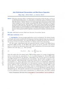
library("JADE") library("BSSasymp") ICAsim jade plot.ts(bss.components(jade), nc = 1, main = "JADE solution") In Figure 5 it can be seen that the first three components are related to the mother’s heartbeat and the fourth component is related to the fetus’s heartbeat. Since we are interested in the

25


−4 −2 −6 2 0 2 4 0 2 4 6 −4 −2 0 1 −1 1 −1 −3

IC.8

3−3

IC.7

3 −6

IC.6

2 −4

IC.5

IC.4

−2 0

IC.3

4

6 −10

IC.2

2 −8

IC.1

0 2

JADE solution

0

500

1000

1500

2000

2500

Time

Figure 5: The independent components estimated with the JADE method. fourth component, we pick up the corresponding coefficients from the fourth row of the unmixing matrix estimate. For demonstration purposes, we also derive their standard errors in order to see how much uncertainty is included in the results. These would be useful for example when selecting the best BSS method in a case where estimation accuracy of only one component is of interest, as opposed to Example 2 where the whole unmixing matrix was considered.

26


R> R> R> R> R>

ascov R> R> R> R> R>

w