Author manuscript, published in "6th International Conference on Field and Service Robotics - FSR 2007, Chamonix : France (2007)"
Outdoor Radar Mapping Using Measurement Likelihood Estimation John Mullane, Martin D. Adams, Wijerupage S. Wijesoma
inria-00196151, version 1 - 12 Dec 2007
Nanyang Technological University School of Electrical and Electronic Engineering 50 Nanyang Avenue, Singapore 639798
[email protected],
[email protected],
[email protected] Summary. This paper fuses target detection and occupancy mapping theory to develop an improved method for outdoor mapping with a radar sensor. It is shown that the occupancy mapping problem is directly coupled with the signal detection processing which occurs in a range sensor, and that the required measurement likelihoods are those commonly encountered in both the target detection and data association hypotheses decisions. The classical binary Bayes filter approach generally treats these measurement likelihoods as fully known deterministic values. From examination of radar detection theory it is shown these likelihoods are only deterministic under a number of unrealistic assumptions which make it impractical for a real radar system used in a outdoor environment. An algorithm is therefore presented which jointly estimates the measurement likelihoods of each target in the environment and uses a particle filter to propagate their corresponding occupancy estimates. The ideas presented in this paper are demonstrated in the field robotics domain using a millimeter wave radar sensor, and comparisons with laser based maps as well as previous radar models are shown.
1 Introduction Autonomous outdoor navigation is still a very active topic of research due to the presence of unstructured objects and rough terrain in realistic situations. For range/bearing sensors commonly used in robot navigation, such as the polaroid sonar or SICK laser, the target detection algorithm is performed internally resulting in a single (r, θ) output to the first signal considered detected. No other information is returned about the world along the bearing angle θ, however it is typical in the case of most sensor models to assume empty space up to range r. This signal may or may not correspond to a target, depending on the environmental properties. These ambiguities are typically resolved in the data association stage by applying a threshold to some statistical distance metric based on the covariance of the predicted and observed feature locations.
2
John Mullane, Martin D. Adams, Wijerupage S. Wijesoma
However, sensor noise in range/bearing measuring sensors is in fact 3 dimensional as an added uncertainty exists in the detection process itself. This observation is not new and is readily considered in such mapping techniques as occupancy grids [1]. For most occupancy grid maps, the occupancy is distributed in a Gaussian manner as a function of the returned range resulting in discrete observations of occupancy in each cell. The discrete Bayes filter is then used as a solution, which is possible as it uses a completely known occupancy measurement model to update the posterior of the occupancy random variable. However, this is not the case for sensors such as the frequency modulated continuous wave (FMCW) radar1 where the occupancy measurement models can be estimated directly. FMCW radar sensors are typically applied to outdoor sensing applications as they can operate in hazardous environments where other sensors will fail. This is due to the radar’s ability to penetrate dust, fog, and rain [2].
inria-00196151, version 1 - 12 Dec 2007
2 Related Work Signal processing problems are not new to the field of autonomous mapping but are generally treated in a simplified manner. In the underwater domain, sonars also return a power versus range vector which is difficult to interpret. In his thesis [3], S. Williams outlined a simple target detection technique for autonomous navigation in a coral reef environment. A constant noise power threshold is used and the maximum signal to noise ratio is chosen as the point target. Clearly this method of extraction results in a large loss of information, which is not desirable for the construction of well defined maps. S. Majumder attempts to overcome this loss by fitting a sum of Gaussian probability density function to the raw sensor data [4], however this represents a likelihood distribution in range of a single point target which is misleading as the data can contain multiple targets, leading to the association of non-corresponding points. In field robotics, standard noise power thresholding2 was again used by S. Clark [5] using an FMCW radar. The range and bearing covariances were then modeled and propagated through an extended Kalman Filter framework to perform autonomous map building (and localisation). This paper further explores the role of signal detection algorithms in autonomous mapping. Section 3 outlines the general occupancy mapping problem, showing how the occupancy variable becomes directly observable when target detection theory is considered. The problems with a discrete Bayesian filter solution are also discussed. Section 3.1 then outlines the estimation of these likelihoods for the radar sensor. Section 4 then proposes a method of 1
2
Due to the modulating techniques, a fast fourier transform can be used to return a power value at discrete range increments. Range resolution, beamwidth, and maximum range are dependant on the particular sensor. Fixed threshold detection is indeed the optimal detector in the case of spatially uncorrelated and homogenous noise distributions of known moments.
Outdoor Radar Mapping Using Measurement Likelihood Estimation
3
estimating the posterior of each occupancy random variable, using a particle filter to propagate samples from both the prior and measurement likelihoods. Section 5 presents some results of the proposed method using real radar data collected from outdoor field experiments, comparisons are made to occupancy maps generated by SICK laser range finders and previously proposed radar mapping algorithms.
3 Grid Mapping Occupancy grid mapping is generally solved by assuming each grid cell to be independent so that the occupancy variable in each cell can independently estimated [1]. Update rules are well established for both probabilistic (Θ = {O, E}) [6] and evidential (Θ = {O, E, U })) frameworks [7],
inria-00196151, version 1 - 12 Dec 2007
log
P (O|z t ) P (O|zt ) 1 − P (O) P (O|z t−1 ) = log + log + log (1) 1 − P (O|z t ) 1 − P (O|zt ) P (O) 1 − P (O|z t−1 ) P mk (X1 )mm (X2 ) X1 ∩X2 =X3 P m(X3 ) = (2) 1− mk (X1 )mm (X2 ) X1 ∩X2 =∅
with O,E and U denoting occupied, empty and unknown estimates respectively. Also, in eqn 2, mk (·) and mm (·) represent mass functions respectively containing the sensor and prior evidences in support of each hypothesis, {X1 , X2 , X3 } ⊂ Θ. These approach requires inverse models, P (O|zt ), which lack rigorous mathematical foundation and may result in inconsistent maps [6]. The measurement likelihood, P (zt |O), is also used [8] along with the common Bayesian update rule, P (O|z t ) = γP (zt |O)P (O|z t−1 )
(3)
where γ is the normalizing constant. The most common model uses the detected range, d, and a Gaussian spread functions with the sensor range covariance, σ 2 . In the case of a 1D the measurement likelihood is written as, p(zt |O) = √
1 2πσ 2
e
(zt −d)2 2σ 2
.
(4)
A key observation is that in this model, the measurement zt is a range reading. The range at which a sensor reports the presence of a landmark can be used in the filtering of its location estimate and does not provide a measurement of the occupancy random variable. To correctly formulate the occupancy estimation problem, the measurement zt should be redefined as zt ∈ {Detection, N o Detection}. A simple expansion of eqn 3 shows how the occupancy measurement likelihoods can be obtained when the signal processing stage is considered. Consider the probability of occupancy given a history of measurements,
4
John Mullane, Martin D. Adams, Wijerupage S. Wijesoma
P (O|z t ).
(5)
t
The measurement history z can now be considered as a sequence of detec¯ We can then expand about both measurement tions, D or non-detections, D. possibilities to get, P (O|zt = D, z t−1 ) ∝ P (zt = D|O)P (O|z t−1 ) ¯ z t−1 ) ∝ P (zt = D|O)P ¯ P (O|zt = D, (O|z t−1 )
(6) (7)
These equations calculate, in closed form, the statistically correct posterior of the occupancy random variable, where the measurement likelihoods ¯ ¯ P (zt = D|O), P (zt = D|E), P (zt = D|O) and P (zt = D|E) are common in target detection algorithms. In real radar systems, these measurement likelihoods have to be estimated online therefore stochastic filtering is required. The following section outlines the measurement likelihood estimation process for a radar sensor.
This section uses radar target detection theory to estimate the measurement likelihoods, p(zt = D|O) and p(zt = D|E). The measurement data is assumed to consist of a vector of K consecutive (in time or range) independent signal intensity measurements, x, for each bearing angle, such as that shown in figure 1. A priori signal distribution assumptions are made on both p(x|Ω O , O) and
15
Targets
Multi-path
10 5
Power (dB)
inria-00196151, version 1 - 12 Dec 2007
3.1 Measurement Likelihood Estimation
0 −5 −10 −15 −20 −25
Clutter free noise 0
50
100
150
200
Range (m)
Fig. 1. A sample spectrum from a frequency modulated continuous wave radar containing K signal intensities in K range bins. Each measurement is assumed to be a single uncorrelated sample from one of the signal distributions shown in figure ??.
p(x|Ω E , E), whereas the distribution moments Ω O and Ω E are unknown and must be estimated. Estimating the False Alarm Likelihood Assuming p(x|Ω E , E) to be exponentially distributed, constant false alarm rate (CFAR) detectors maintain the pre-defined p(zt = D|E) if the K consecutive intensity measurements are independent samples from identically and
Outdoor Radar Mapping Using Measurement Likelihood Estimation
5
independently distributed p(x|Ω E , E) and more importantly, given that the distribution assumption on p(x|Ω E , E), is valid. The density of equation 19 will thus become deterministic. Estimating the Detection Likelihood
inria-00196151, version 1 - 12 Dec 2007
Signal detection literature generally considers the probability of detection for targets of known SNR, whereas this work requires p(zt = D|O) to be estimated with an unknown SNR. Therefore an estimate of the targets mean SNR, S¯ is required. There are numerous adaptive methods of generating local estimates of the unknown noise distribution parameters [9]. Thus, given an estimate of the local noise intensity from the CFAR detector, {x|E} S¯ can be estimated as, {x|O} − {x|E} S¯ = . (8) {x|E} An ordered-statistics approach [10], which is adopted in this work, has been shown to be most robust in situations of high clutter and multi-target situations, as is commonly encountered in a field robotics environment. Closed form solutions then exist for p(zt = D|O), µ ¶−N T {x|E} p(zt = D|O) = 1 + (9) 1 + S¯ with, 1 exp(−x/µ) µ µ r ¶ ¡ ¢ 1 sx p(x|Ω O = {µ, s}, O) = exp (−x/µ) + s )I0 2 µ µ 2s ¯ = ¯ p(s|S) exp(−s2 /S). S¯ p(x|Ω E = µ, E) =
By approximating each estimate as a Gaussian random variable, we can generate a Gaussian distributed estimate of p(zt = D|O). These likelihoods are then used during the occupancy measurement update as seen in equation 18 in the following section.
4 The Occupancy Filter This section outlines the formulation for the filtering of an occupancy random variable using the measurement likelihood estimates. The objective of this filter is to propagate the posterior density of the occupancy variable, O. As this estimation is now modeled by a density function rather than a discrete random variable, the goal is to propagate the density3 , 3
As opposed to a deterministic value in the binary Bayes filter.
6
John Mullane, Martin D. Adams, Wijerupage S. Wijesoma
p(O|z t ).
(10)
We can expand eqn 10 as before to get, p(O|z t ) = γp(zt |O)p(O|z t−1 ).
(11)
A static process model is assumed such that, p(Ot |Ot−1 ) = p(O|z t−1 ).
(12)
inria-00196151, version 1 - 12 Dec 2007
This assumption is inline with standard autonomous mapping algorithms where a static state is assumed, thus no change occurs to its occupancy estimate during the time update. As the true value of the occupancy state, O, is Boolean we must have the constraint, Z Z p(O|z t ) + p(E|z t ) = 1. (13) Thus, given two distributions p(zt = D|O) and p(zt = D|E) from the measurement likelihood estimator, as well as the two priors p(O|z t−1 ) and p(E|z t−1 ) we can proceed to estimate the posterior, p(O|z t ). The algorithm proceeds as, 1. Draw Nr samples, Or , from one of the prior existence densities, Or ∼ p(O|z t−1 ), and, with,
r ∈ {1 . . . Nr }
(14)
E r = 1 − Or
(15)
p(O|z 0 ) = U (0, 1).
(16)
2. Uniformly weight the sets of particles, r wM =
1 , ∀r ∈ {1 . . . Nr }, M ∈ {O, E}. 2Nr
(17)
Thus the weights for the combined set of particles Or and E r are norr malized. Therefore p(O|z t ) is approximated by the set {(Or , wO }, p(E|z t ) r r is approximated by the set {E , wE } ∀r = {1 . . . Nr }, and the discrete form of equation 13 is satisfied. 3. Draw Nl samples from the measurement likelihood distributions i.e the detection and false alarm densities. The general assumption that p(zt = D|O) = 1 − p(zt = D|E) [1] is not valid and independent samples must be drawn. l zO ∼ p(zt = D|O) l zE
∼ p(zt = D|E),
(18) l ∈ {1 . . . Nl }.
(19)
Outdoor Radar Mapping Using Measurement Likelihood Estimation
7
4. Weight the measurement likelihood particles according to, 1 p(zt = D|O) Nl 1 l v˜E = p(zt = D|E) Nl l v˜O =
(20) (21)
and normalize, v˜l l vO = PNlO l vE =
j=1 j v˜E PNl j=1
j v˜O
j v˜E
(22) (23)
inria-00196151, version 1 - 12 Dec 2007
l l l l to generate the two sets of particles and weights {zO , vO } and {zE , vE } ∀l = {1 . . . Nl } which then approximate both measurement likelihoods.
5. Convolve both sets of measurement likelihood and prior particles through the deterministic Bayesian update rule in equations 6-7 to generate a superset of posterior particles {Θk , Ψ k } with k ∈ {1 . . . Nr Nl }, Θk = Ψk =
l zO Or l Or + z l E r zO E
(24)
l r vO wO l r l wr vO wO + vE E
(25)
where r ∈ {1 . . . Nr } and l ∈ {1 . . . Nl } as before. 6. Resample the superset {Θk , Ψk }, reducing the sample number back down to Nr which, due to the static process model assumption, then give a particle approximation of the prior density, p(O|z t ), at time t+1. By virtue of the Bayesian normalizing factor, the posterior occupancy particles are guaranteed to exist only within the bounded range [0,1].
5 Experiments The first example propagates an occupancy variable in each range bin of the radar (K = 800) at a single bearing angle. A sample spectrum from this data was shown previously in figure 1, with three target signals present. Mixing these samples with the prior samples and resampling according to equations 18 - 25, we get the posterior density samples in each range bin as seen in figure 3. The figure also shows the corresponding variance estimated for the
8
John Mullane, Martin D. Adams, Wijerupage S. Wijesoma
occupancy variable. Figure 4 shows the same corresponding plots after 5 iterations, along with update variance in each range bin. It can be seen that the variance remains practically zero for most cells however due to high variance measurement likelihood estimates, particulary at 5m and 150m, there remains some uncertainty in the occupancy estimate. Previous models using deterministic updates fail to account for this uncertainty. A two dimensional map is shown in figure 5 where multiple radar scans are fused in a carpark environment. For comparison purposes an occupancy map built by a laser is included. The result shows promising map building capability using this radar model. Measurement Samples 1 0.9
0.7 0.6 0.5 0.4 0.3 0.2 0.1 0
0
50
100
150
200
Range (m)
Fig. 2. The measurement samples based on the estimated probability of detection and the output hypothesis of the detector. Samples represent particle approximations of p(zt = D|O) or p(zt = D|E), in the case of H1 and H0 hypotheses respectively. Larger spreads of particles indicate increased uncertainty in that cell. The dashed plot represents the mean value of Pd in each range bin, independent of the detection hypothesis, thus accommodating for potential missed detections.
Posterior Samples
Posterior variance
1
0.16
0.9
0.14
0.8 0.12 0.7
p(O|z)
inria-00196151, version 1 - 12 Dec 2007
Detection Likelihood
0.8
0.6
0.1
0.5
0.08
0.4
0.06
0.3 0.04 0.2 0.02
0.1 0
0
50
100
Range (m)
150
200
0
0
50
100
150
200
Range (m)
Fig. 3. The left hand figure shows the posterior existence samples after a single filter iteration, with the dashed line representing the mean occupancy in each bin. The right hand figure shows the corresponding variance of the estimates in each range bin.
Outdoor Radar Mapping Using Measurement Likelihood Estimation Posterior Samples
9
Posterior variance
1
0.12
Probability of Existence
0.9 0.1
0.8 0.7
0.08 0.6 0.5
0.06
0.4 0.04
0.3 0.2
0.02 0.1 0
0
50
100
150
200
0
0
50
Range (m)
100
150
200
Range (m)
Fig. 4. The left hand figure shows the posterior occupancy samples, after five filter iterations, with the dashed line again representing the mean existence in each bin. Updated variances are shown in the right hand figure.
Entrance Passage
Main Building Wall
Trees Trees
Entrance Passage Range (m)
inria-00196151, version 1 - 12 Dec 2007
Low wall Main Building Wall
Fig. 5. The left hand figure shows an overview of testing ground (Cars were absent at time of experiment). The center figure shows the occupancy map using the radar sensor and the proposed algorithm. The right most figure shows the corresponding map constructed using laser data and an arbitrary sensor model. Highlighted are some landmarks which are detected by the radar but missed by the laser. This is mainly due to the radars increased beamwidth.
6 Conclusion This paper discussed the role played by target detection algorithms in autonomous outdoor mapping. It was shown that the measurement likelihoods used to propagate the occupancy estimate are assumed known in previous mapping sensor models. Once this assumption is relaxed, the measurement likelihoods become stochastic estimates based on the signal detection algorithm and the measurement intensity information. A particle filter approach
10
John Mullane, Martin D. Adams, Wijerupage S. Wijesoma
to the occupancy estimation problem was then proposed. This concept was demonstrated for an FMCW radar sensor which is typically used in an outdoor environment. For most practical scenarios Pd À Pf a , thus Bayesian based mapping method will assign almost unity occupancy to any detection. However, when the assumption on the noise distribution is violated and Pf a deviates from its theoretical value, an evidential method should be applied as there would be large ambiguity as to the true false alarm probability. This would further improve the mapping accuracy. Further work also would integrate three dimensional uncertainties (in Euclidean location as well as occupancy) into data association decisions and SLAM algorithms.
Acknowledgements
inria-00196151, version 1 - 12 Dec 2007
This work was funded under the second author’s AcRF Grant, RG 10/01, Singapore.
References 1. H. Moravec and A.E. Elfes. High resolution maps from wide angle sonar. In Proceedings of the 1985 IEEE International Conference on Robotics and Automation, pages 116–121, March 1985. 2. G. Brooker, M. Bishop, and S. Scheding. Millimetre waves for robotics. In Australian Conference for Robotics and Automation, Sidney, Australia, November 2001. 3. S. Williams. Efficient Solutions to Autonomous Mapping and Navigation Problems. PhD thesis, Australian Centre for Field Robotics, University of Sydney, 2001. 4. S. Majumder. Sensor Fusion and Feature Based Navigation for Subsea Robots. PhD thesis, The University of Sydney, August 2001. 5. S. Clark and H.F. Durrant-Whyte. Autonomous land navigation using millimeter wave radar. In International Conference on Robotics and Automation (ICRA), pages 3697–3702, Leuven,Belgium, May 1998. IEEE. 6. S. Thrun. Autonomous robots. volume 15, pages 111–127, 2003. 7. D. Pagac, E. Nebot, and H.F. Durrant-Whyte. An evidential approach for map building for autonomous vehicles. IEEE Transactions on Robotics and Automation, vol. 14(4), August 1998. 8. K. Konolige. Improved occupancy grids for map building. Auton. Robots, 4(4):351–367, 1997. 9. H. Rohling. Some radar topics: Waveform design, range (cfar) and target recognition. In NATO: Advances in Sensing with Security Applications, Il Ciocco, Italy, July 2005. 10. H. Rohling and R. Mende. OS CFAR performance in a 77 GHz radar sensor for car applications. In CIE International Conference of Radar, pages 109 – 114, October 1996.