program takes advantage of processing accomplished by PROC MIXED and some SAS/IML® ... Taking advantage of PROC MIXED, ODS and SAS/IML®, I present a macro program to conduct the parametric ..... Email: [email protected].
University, Stillwater, OK ... Build a data mining model, which will predict whether a user may become an ..... Advertising, Journal of Business Research, etc.
contain sets of fields to accommodate the maximum number of replicates in the ..... CCBB 23. C. 2. CNB. 6600. 24. C. 3. CCB. CCCB 24. C. 3. CNB. 6700. 25. C ... MERGE includes a RENAME option employing AddX, a macro variable defined ...
TTC PD drives RWA and as such it is important to have the correct PD level to .... In cases where at least one default was observed one can use MLE to get estimates ... The multiple integrals have to be estimated using Monte Carlo simulation.Missing:
patients by estimating their probability of being readmitted within 30 days of .... More formerly, CMS hired Yale New Haven Health Services .... Align business and technical resources with a common vocabulary to accelerate new initiatives .... It is
Raval AD,Sambamoorthi U: Incremental Healthcare Expenditures Associated with Thyroid. Disorders among ... Email: [email protected]. SAS and all other ...
Centre for Business Mathematics and Informatics ... in realised PDs, LGDs and EADs from expectations become significant enough to call the validity.
Asish Satpathy, School of Business and Administration, University of ... Facebook about a particular topic of their interests, these opinions can be highly .... Marketing, Journal of Advertising Research, Journal of Advertising, Journal of Business .
SCW on the basic, un-tuned Lustre were not optimal. By default, tunable Lustre parameters ..... Email: [email protected]. SAS and all other SAS Institute ...
660 Rosedale Road â Mail Stop 20-T. Princeton, NJ 08541. Telephone: 609-734-1989. Email: [email protected]. TRADEMARKS. SAS and all other SAS Institute Inc.
provide a better fit of survey items into survey domains. ... survey items to construct domains. .... 4F[Concept domain name] is how we labeled our factors.
other analytical software such as R or Matlab, the IML language is intuitive to use. ... in IML can be easily output to SAS Datasets for use in existing analytic or ...
Location Based Association of Customers' Sentiments and Retail Sales ... with their locations, number of employees, sales volume (2014) information gathered .... We thank the SAS Global forum 2015 conference committee for providing a ...
big data transformation capabilities for Hadoop. ⢠integration with the SAS® LASR⢠platform. ⢠enhanced features
recent years, particularly within the field of complex survey data analysis. ..... Perhaps the most popular form of the
Reject Inference Techniques Implemented in Credit Scoring for SAS® ..... characteristic variables were rejected if their relationship could not be explained.
Apr 28, 2015 - surveys to research participants, and prevented withdrawn participants from receiving scheduled emails. In this paper, we demonstrate how to ...
options available to survey researchers in the handling of missing and ânot applicableâ survey .... 4F[Concept domain name] is how we labeled our factors.
Some variables, for example weight, race, and encounter ID contained anomalies such as questions marks and .... Advertising Research, Journal of Advertising, Journal of Business Research, etc. ... Email: [email protected].
application, Tractor Supply Company (TSC) engaged SAS® Institute to deliver a fully integrated forecasting solution that promised a significant improvement of ...
Available support.sas.com/rnd/scalability/grid/gridfunc.html. Tran, A., and R. Williams, 2002. âImplementing Site Poli
ODBC Driver â The ODBC driver submits SQL statements to the specified data source and .... Determining the Version Num
Using SAS/STAT® Software to Validate a Health Literacy Prediction Model .... Data analysis was conducted using SAS/STAT® 9.4; statistical significance assessed as ..... Validation of screening questions for limited health literacy in a large.
Email: [email protected]. Phone: +86 10-8319-3355. SAS and all other SAS Institute Inc. product or service names are registered trademarks or trademarks of.
due to violation of their basic assumption. ... SAS® software. .... the release of version 9.4 of SAS software, Fine and Gray's sub-distribution hazard model can be.
Paper 1424-2015
Competing risk survival analysis using SAS® When, why and how Lovedeep Gondara, University of Illinois Springfield ABSTRACT Competing risk arise in time to event data when the event of interest cannot be observed because of a preceding event i.e. a competing event occurring before. An example can be of an event of interest being a specific cause of death where death from any other cause can be termed as a competing event, if focusing on relapse, death before relapse would constitute a competing event. It is well studied and pointed out that in presence of competing risks, the standard product limit methods yield biased results due to violation of their basic assumption. The effect of competing events on parameter estimation depends on their distribution and frequency. Fine and Gray’s sub-distribution hazard model can be used in presence of competing events which is available in PROC PHREG with the release of version 9.4 of SAS® software. .
INTRODUCTION Competing event can be considered as an alternative outcome that makes the observation of primary or outcome of interest impossible. Standard survival analysis concentrates on only one type of failure in time to event data i.e. it usually censors failures due to other causes which yields biased results. Cumulative incidence estimate proposed by Kalbfleisch and Prentice [10] can be used as a remedy. 𝑡
𝐼𝑗 (𝑡) = ∫ 𝑓𝑗 (𝑢)𝑑𝑢 = Pr{𝑇 ≤ 𝑡&𝐽 = 𝑗} 0
Which represents the probability that an event of type j has occurred by time t. Following two approaches can be used for introducing covariates in context of competing risks: 1. Apply a cox proportional hazard model to cause specific hazards 2. Use model proposed by Fine and Gray [1] that focuses on cumulative incident function , ̅̅̅̅ 𝜆̅𝑗 (𝑡, 𝑥) = 𝜆 𝑗0 (𝑡)exp{𝑥 𝛽𝑗 }
Where
̅̅̅̅ 𝜆𝑗0 (𝑡) is the baseline sub hazard for events of type 𝑗 exp{𝑥 , 𝛽𝑗 } is the relative risk associated with covariates 𝑥 The partial likelihood of the sub-distribution hazard model was defined by Fine and Gray as 𝑟
𝐿(𝛽) = ∏ 𝑗=1
exp(𝑥𝑗 𝛽) ∑𝑖𝜖ℜ𝑗 𝑤𝑗𝑖 exp(𝑥𝑖 𝛽)
Where 𝑥𝑗 is the covariate row vector of the subject experiencing an event of interest at 𝑡𝑗 .
1
The risk set ℜj is defined as
ℜ𝑗 = {𝑖; 𝑡𝑖 ≥ 𝑡 ∨ (𝑡𝑖 ≤ 𝑡 ∧ 𝜖𝑖 = 2)} And it includes the individuals who at time t are at risk of event of interest and anyone who had a competing event before time t. Time and subject specific weights are used when censoring occurs. Subjects at risk from event of interest (type 1) at time t and who have not witnessed a competing event before t have equal weights (𝑤𝑖 = 1) and for subjects with competing event at ti < t weights are given as 𝑤𝑖 < 1. Weights for Fine and Gray’s model can be calculated as
1𝑖𝑓𝑡𝑖 ≥ 𝑡 ̂ 𝐺 (𝑡) 𝑤𝑗𝑖 = { 𝑖𝑓𝜀𝑖 = 2 ∧ 𝑡𝑖 < 𝑡 𝐺̂ (𝑡𝑖 ) Where 𝐺̂ (t) denotes estimator of the censoring distribution i.e. cumulative probability of still being followed up at time t. It can be estimated by usual product limit method by reversing the meaning of censoring indicator.
WHEN? Competing risk survival analysis should be considered when the observation of event of interest is made impossible by a preceding competing event, e.g. In case of oncology competing risks are encountered when patients are followed after treatment, and their first failure event may be local recurrence, distant metastases, onset of second primary cancer, or death precluding these events. So if event of interest is any type of relapse, then the observation of this event is made impossible by death preceding relapse. It can be argued that competing risk models provide real world probabilities of death when competing events are present as opposed to standard survival models by allowing us to separate the probability of event into different causes.
Figure1. Competing risk scenario
2
Figure 1 simulates a cohort including competing events, where event of interest can be considered as cancer but its observation is made impossible in case 6 & 8 by a preceding competing event. Figure 2 shows systematic application of diminishing weights ( 𝑤𝑖 ) to these cases after occurrence of competing events, which are calculated by reversing the indicator definition using standard product limit methods.
Figure 2. Application of weights for competing events
WHY? It has been frequently pointed out that in presence of competing events, standard product limit method of estimating survivor function for event of interest yields biased results as the probability of occurrence is modified by an antecedent competing event. We use examples below to support this point.
DATA We use the BMT dataset presented by Klein and Moeschberger(1997) [6] which contains data for bone marrow transplant for 137 patients, grouped into three risk categories based on their status at the time of transplantation: acute lymphoblastic leukemia (ALL), acute myelocytic leukemia (AML) low-risk, and AML high-risk. During the follow-up period, some patients might relapse or some patients might die while in remission. Consider relapse to be the event of interest. Death is a competing risk because death impedes the occurrence of leukemia relapse.
3
SCENARIO 1. RARE COMPETING EVENTS Data was altered to change the frequency and distribution of competing events with most competing events occurring at a later time period. Summary of events of interest, competing events and censoring is given in table below. Event
Frequency
1 (Event of interest)
77
2 (Competing event)
6
0 (Censored)
54
Table 1. Event distribution for dataset with sparse competing events
Two models were fit to this data, one being the Cox proportional hazard model in which all competing events are censored and second using Fine and Gray’s sub-distribution hazard model. Comparisons of both models and CIF plot are given below. Covariate