Paper 3300-2015
An Empirical Comparison of Multiple Imputation Approaches for Treating Missing Data in Observational Studies Patricia Rodríguez de Gil, Jeffrey D. Kromrey, Rheta E. Lanehart, Eun-Sook Kim, Jessica Montgomery, Yan Wang, Reginald Lee, Chunhua Cao, Shetay Ashford University of South Florida ABSTRACT Missing data are a common and significant problem that researchers and data analysts encounter in applied research. Because most statistical procedures require complete data, missing data can substantially affect the analysis and the interpretation of results if left untreated. Methods to treat missing data have been developed so that missing values are imputed and analyses can be conducted using standard statistical procedures. Among these missing data methods, Multiple Imputation has received considerable attention and its effectiveness has been explored, for example, in the context of survey and longitudinal research. This paper compares four Multiple Imputation approaches for treating missing continuous covariate data under MCAR, MAR, and MNAR assumptions in the context of propensity score analysis and observational studies. The comparison of four Multiple Imputation approaches in terms of bias and variability in parameter estimates, Type I error rates, and statistical power is presented. In addition, complete case analysis (listwise deletion) is presented as the default analysis that would be conducted if missing data are not treated. Issues are discussed, and conclusions and recommendations are provided.
INTRODUCTION Researchers and statistical data analysts encounter many issues but those associated with missing data often are the most pressing. Missing data are a common problem in many areas of applied research because conventional statistical procedures and software assume complete data (Allison, 2001). Missing data problems (e.g., biased estimates, loss of statistical power) that result when data are missing for some observations have been studied for many years. After missing data have been treated with deletion and imputation approaches, researchers can proceed to conduct the computations using standard statistical methods for analyzing complete data. Among the several methods developed to deal with missing data problems, Multiple Imputation (MI) has become one of the most accepted methods. If its assumptions are met, MI has shown excellent qualities (see, for example, reviews by Graham & Hofer, 2000; Schafer & Graham, 2000; Schafer & Olsen, 1998). Because the properties of the observed data and the missing data might be different, when applying a missing data treatment (MDT), e.g., MI, the process or mechanism that causes missingness might need to be incorporated into the statistical model, the advantage being that incorporating the missing data mechanism leads to efficient data modeling for fitting the data adequately. Rubin’s (1976) theoretical framework is the most widely accepted for missing data research.
RUBIN’S (1976) MISSING DATA TAXONOMY As Rubin (2005) stated, the MDT should reflect the underlying uncertainty of the process or mechanism that best explains why data are missing. Let Y = (Y1, Y2,…,Yp) be a random vector variable for p-dimensional multivariate data (y x p matrix), and θ and δ are the parameter of the data and the parameter of the conditional probability of the observed pattern of missing data, respectively. In the presence of missing data, φ, inferences about θ are conditional on δ, the mechanism that causes missingness. That is, given the data at hand, the purpose of the missing data process is to allow making valid inferences about θ but these inferences depend upon or are conditional on δ, the mechanism that generated missing data:
Missing Completely at Random (MCAR). When the probability of a missing value on a variable is independent of the observed or unobserved value for any variable, that is, the probability that yi is
1
missing is independent of the probability of missingness for any yj, data are missing completely at random or MCAR.
Missing at Random (MAR). When the probability that yi is missing for variable Y is dependent on the data of any other variables but not on the variable Y of interest, data are missing at random or MAR. In addition, MAR requires data on a variable to be missing randomly within subgroups (Roth, 1994).
Missing NOT at Random (MNAR). When the probability of a missing value depends on unobserved data or data that could have been observed, data are missing not at random or MNAR. That is, the value of yi depends on the value of Yi. Under this scenario, why data are missing is not ignorable, thus requiring that the missing data mechanism is modeled to make valid inferences about the model parameter.
OBSERVATIONAL STUDIES Randomized trials are the “gold standard procedure” for evaluating the effectiveness of treatment effects; under random assignment to T (t1 = treatment, t0 = control), xi is the vector of baseline covariates (i.e., pretreatment measurements, before treatment is assigned) for which the i observations or units are likely to be similar. Thus, in a randomized experiment, every observation has the same probability of assignment to either t1 or t0 independently of x (strong ignorability of assignment assumption) and the average treatment effect is directly estimated as, τ = E(y1 ) – E(y0), where E = the expectation in the population.
When an experimental study (randomized trial) cannot be conducted because of, for example, ethical issues (e.g., assignment of observations to life-threatening conditions), nonrandomized or observational studies provide the necessary data from which treatment effect inferences can be made. Because in these nonrandomized studies the treatment group (t1) and the control group (t0) can differ systematically in the baseline covariates due to selection bias, researchers can apply methods that ensure that selection bias is corrected; otherwise, biased estimates of the treatment effects might result. One of these methods to handle the differences between treatment group and control group in an observational study is propensity score (PS) analysis.
CAUSAL INFERENCE: THE ROLE OF THE PS IN OBSERVATIONAL STUDIES Rosenbaum and Rubin (1983) defined the propensity score as “the conditional probability of assignment to a particular treatment given a vector of observed covariates” x (p. 41). That is, the PS allows the conditional assignment of units to treatment and control groups given x. Let Z (z1 = 1) be the probability of assignment to the treatment effect conditional on x; the true PS is estimated as: pr(𝑧 = 1 | 𝑥) =
pr(𝑧 = 1) pr(𝑥|𝑧 = 1) . pr(𝑧 = 1) pr(𝑥 |𝑧 = 1) + pr(𝑧 = 0) pr(𝑥|𝑧 = 0)
In practice, it is not possible for any observation or unit to receive both treatments; either yi1 or yi0 is observed and a unique response yit is expected (stable unit-treatment value assumption; Rubin,2005).
APPLICATION OF MULTIPLE IMPUTATION TO OBSERVATIONAL STUDIES The PS is an important application in observational studies because it adjusts for confounding variables which are a source for potential bias in treatment effect estimates. Thus, conditioning on the PS (e.g., matched sampling, pair matching, adjustment by subclassification, and covariance adjustment) can provide unbiased estimates of the average treatment effect (ATE). Multiple imputation (MI) is a multiple imputation procedure that creates m imputed data sets for an incomplete p-dimensional multivariate data. That is, missing values are replaced with a set of plausible values that represent a random sample and thus representing the uncertainty about the missing value.
2
METHOD Using simulation methods, this factorial study was conducted to compare the performance of PROC MI for missing continuous covariate data under ignorable and nonignorable missing data mechanisms in the context of propensity score analysis and observational studies. Data were generated using the IML procedure, then analyzed using the MI, MIANALYZE, and REG procedures. EXPERIMENTAL FACTORS The experimental factors related to the study design included sample size (500, 1000), treatment effect magnitude (0, .05, .10, .15), correlation between covariates (0, .5), and number of covariates (15, 30). The factors related to missing data included the missing data mechanism (MCAR, MAR, MNAR), proportion of missing observations (.20, .40, .60), proportion of missing covariates (.20, .40, .60), and missing data treatment (Multiple Imputation and Complete-Case Analysis). An analysis of the samples with no missing data was conducted for comparison. MULTIPLE IMPUTATION MODELS Incomplete data were treated using the following MI models: 1. Cov Only (MI). Imputing Missing Covariates Only - Separate PS Analysis. PROC MI is implemented to impute missing covariates only; then the PS is estimated on each imputed data set. Treatment effect estimation with PS ANCOVA is conducted on each imputed data set separately and then combined across imputed data sets. The following SAS code imputes missing covariates proc mi noprint data=missing out=imputed1; title 'PROC MI to Impute Covariates Only';
Then, PS is estimated on imputed data sets: proc logistic descending data = imputed1; model group = X1 - X30; by _imputation_; output out= ps1 PREDICTED = ps_pred; title 'Propensity Score Estimation on Imputed Covariates'; run;
Treatment effects ON EACH imputed data set are estimated using PS ANCOVA: proc reg data = ps1 outest = outreg covout; model Y = ps_pred group / CLB; by _imputation_; title 'Treatment Effect Estimation on Each Imputed Data Set'; run;
Lastly, treatment effects are combined across imputed data sets: proc mianalyze data=outreg; modeleffects intercept group ps_pred; ods output parameterestimates=out_method1; title 'Method #1 Treatment Effect Estimates (Imputed Covariates, Separate Analyses)'; run;
2. Cov Only (Avg). Imputing Missing Covariates Only – Mean PS Analysis. PROC MI is implemented to impute missing covariates only; then the PS is estimated on each imputed data set and averaged across imputed data sets for each observation. Treatment effect estimation with PS ANCOVA is then conducted on the data set with mean PS. For this MI model, simulees are assigned to the treatment and control groups and missing covariates are imputed using the same procedures as in method 1. Then, mean PS is computed across imputations for each observation. proc sort data = ps1;
3
by IDN; proc means noprint data = ps1; by IDN; var ps_pred; ID Y group; output out = persons mean = mn_ps_pred;
Treatment effects are estimated with PS ANCOVA on each averaged set: proc reg data = persons; model Y = mn_ps_pred group / CLB; ods output parameterestimates=out_method2; title 'Method #2 Treatment Effect Estimates (Imputed Covariates, Mean PS)'; run;
3. Cov PS (MI). Imputing Missing Covariates and PS – Separate PS Analysis. PS is estimated on complete cases in samples; then PROC MI is implemented to impute both missing covariates and missing PS. Treatment effect estimation with PS ANCOVA is conducted on each separate imputed data set and combined across imputed data sets. Estimate PS on complete cases in samples: proc logistic descending data = missing; model group = X1 - X30; output out= ps2 PREDICTED = ps_pred; title 'Propensity Score Estimation on Complete Cases'; run;
then, impute missing covariates and PS: proc mi noprint data=ps2 out=imputed2; title 'PROC MI to Impute Covariates and PS'; run;
Treatment effects are estimated and combined using the SAS code as in MI Method 1. 4. Cov_PS (Avg). Imputing Missing Covariates and PS – Mean PS Analysis. PS is estimated on complete cases in samples; then PROC MI is implemented to impute both missing covariates and missing PS. The PS is averaged across imputations; then treatment effect estimation with PS ANCOVA is conducted on the data set with mean PS. For MI method 4, PS is imputed using the SAS code as in MI method 3 and PS is averaged using the SAS code as in MI method 2. 5. Complete Case Analysis – Listwise Deletion. PS is estimated on complete cases in samples and treatment effect estimation with PS ANCOVA is conducted. 6. No Missing Data Analysis. PS is estimated for samples prior to the imposition of missing data.
RESULTS MISSING COMPLETELY AT RANDOM (MCAR) Statistical Bias As illustrated in Figure 1, although the mean biases for Cov Only (Avg), Cov PS (MI), and Cov PS (Avg) were not substantial, great variability existed in the bias distribution especially for the Cov Only (Avg) and Cov PS (Avg) approaches. In addition, those two approaches provided underestimation of the treatment effect, while the Cov PS (MI) tended to slightly overestimate the treatment effect. Bias was relatively small for the other two missing data treatments and the complete data conditions, although for listwise deletion, there were cases in which the treatment effect was severely overestimated.
4
Figure 1. Distributions of Bias by Method Across all MCAR Conditions
The number of covariates and covariate intercorrelation had significant impact on the bias estimates (Figure 2). With a larger number of covariates and correlated covariates, the statistical bias increased. 0.40 0.20 0.00 -0.20
Bias
k 15 rx 0 -0.40 k 15 rx 0.5 -0.60 -0.80
k 30 rx 0 k 30 rx 0.5
-1.00 Complete Cov Only (MI) Data
Cov Only (Avg)
Cov + PS (MI)
Method
Cov + PS (Avg)
Listwise
Figure 2. Mean Bias by Number of Covariates and Covariate Intercorrelation for MCAR
RMSE The overall distributions of RMSE for the MCAR conditions are presented in Figure 3. Substantial variability in RMSE is evident for all missing data treatment approaches as well as for the samples before missingness was imposed. In comparing these distributions, the MI approach with covariates only produced only slightly larger RMSE values than those obtained with complete data, while the other three approaches to MI yielded notably larger RMSE values. The listwise deletion approach performed well, providing RMSE values between these extremes.
5
Figure 3. Distributions of RMSE by Method Across all MCAR Conditions
The magnitude of RMSE varied as a function of the number of covariates and the correlation between the covariates (Figure 4). Evident in this figure is that RMSE increases with more covariates and with correlation between the covariates. However, the impact of covariate correlation is greater with a larger number of covariates. In each condition, the MI approach with covariates only produced only slightly larger mean RMSE values than those obtained with complete data.
Mean RMSE
2.50 2.25
k = 15, r = 0
2.00
k = 15, r = 0.5
1.75
k = 30, r = 0
1.50
k = 30, r = 0.5
1.25 1.00 0.75 0.50 0.25 0.00 Complete Data
Cov Only (MI)
Cov Only Cov + PS (MI) (Avg) Method
Cov + PS (Avg)
Listwise
Figure 4. Mean RMSE by Number of Covariates and Covariate Intercorrelation for MCAR
Confidence Interval Coverage The overall distributions of 95% confidence interval (CI) coverage by missing data methods under MCAR are presented in Figure 5. The MI approach with covariates only surpassed the other MI methods in terms of CI coverage. For this outperforming method, there is no noticeable difference from the CI coverage under the complete data conditions. The listwise deletion and Cov PS (MI) also showed reasonable CI coverage around 95% except outlying cases. However, when the treatment effect was estimated with the average propensity scores, the CI coverage was notably below .95 with large variability.
6
Figure 5. Distributions of CI Coverage by Method Across all MCAR Conditions
For the complete data and the MI with covariates only conditions, the CI coverage was near .95 regardless of simulation conditions. For the other methods, the proportion of missing observations generally emerged as a major factor associated with the variability of CI coverage across conditions: the more missing observations, the lower CI coverage (see Figure 6). 1.00
0.2
0.4
0.6
CI Coverage
0.80 0.60 0.40 0.20 0.00 Complete Cov Only (MI) Cov Only Data (Avg)
Cov + PS (MI)
Cov + PS (Avg)
Listwise
Method Figure 6. Mean Confidence Interval Coverage by Proportion of Missing Observations under MCAR
Confidence Interval Width As presented in Figure 7, the overall distributions of confidence interval width were not substantially different across missing data methods and very similar to that of the complete data. The major design factors related to the variability of CI width include the number of covariates, covariate intercorrelation, and the interaction between them. As shown in Figure 8, the width of confidence interval became larger when the number of covariates was 30. The impact of number of covariates on the CI width was noticeably greater when the covariates were correlated each other.
7
Figure 7. Distributions of CI Width by Method Across All MCAR Conditions
7.00 Covariates = 15 r = 0 6.00
Covariates = 15 r = 0.5 Covariates = 30 r = 0
Mean Width
5.00
Covariates = 30 r = 0.5
4.00 3.00 2.00 1.00 0.00 Complete Data
Cov Only (MI)
Cov Only Cov + PS (MI) Cov + PS (Avg) (Avg)
Listwise
Figure 8. Mean Interval Width by Number of Covariates and Covariate Intercorrelation under MCAR
Type I Error Control The overall distributions of Type I error estimates for the MCAR conditions are presented in Figure 9. The MI approach with covariates only, listwise deletion, and complete data evidenced Type I error rates that were adequately controlled, while the other three approaches yielded notably larger Type I error estimates.
8
Figure 9. Distributions of Type I Error Rates by Method Across All MCAR Conditions
The number of covariates and covariate intercorrelation (Figure 10) had significant impacts on the Type I error control of most approaches, although the direction of the impact varied across treatment methods. The MI approach with covariates only was relatively unaffected by these factors.
0.6 k = 15, r = 0
Mean Type I Error Rate
0.5 0.4
k = 15, r = 0.5 k = 30, r = 0 k = 30, r = 0.5
0.3 0.2 0.1 0 Complete Data
Cov Only (MI)
Cov Only (Avg)
Cov + PS (MI)
Cov + PS (Avg)
Listwise
Method Figure 10. Mean Type I Error Rate by Number of Covariates and Covariate Intercorrelation under MCAR
Statistical Power Because statistical power should only be considered after adequate Type I error control has been established, power was estimated only for complete data, listwise deletion, and MI with covariates only. The overall distributions of power for the MCAR conditions with these methods are presented in Figure 11. The complete data condition evidenced the greatest power, but the MI treatment provided power that was nearly as large on average. The listwise deletion approach provided notably lower power.
9
Figure 11. Distributions of MCAR Power Estimates by Method Across MCAR Conditions
MISSING AT RANDOM (MAR) Statistical Bias The overall distributions of bias for the MAR conditions are presented in Figure 12. With complete data, bias was small in all conditions. Among the five approaches for missing data treatment, the MI with covariates only and listwise deletion produced relatively small bias values.
Figure 12. Distributions of Bias by Method Across all MAR Conditions
The magnitude of bias varied as a function of the number of covariates and the percentage of missing covariates (Figure 13). Evident in this figure is that the magnitude of bias increased with more covariates and a higher percentage of missing covariates. However, across levels of these factors, the MI approach with covariates only and listwise deletion provided bias values only slightly greater than the complete data conditions.
10
1.00 0.80 0.60
k = 15, .2 Missing k = 15, .4 Missing k = 15, .6 Missing k = 30, .2 Missing
Mean Bias
0.40 0.20
k = 30, .4 Missing k = 30, .6 Missing
0.00 -0.20 -0.40 -0.60 -0.80 Complete Data
Cov Only (MI)
Cov Only (Avg)
Cov + PS (MI)
Cov + PS (Avg)
Listwise
Method Figure 13. Mean Bias by Number of Covariates and Covariate Intercorrelation for MAR
RMSE The overall distributions of RMSE for the MAR conditions are presented in Figure 14. The results of RMSE under the MAR conditions were very similar to those under the MCAR. However, RMSE was generally larger with MAR. Substantial variability in RMSE was observed for all missing data treatment approaches. The major simulation factors related to the variability of RMSE includes the number of covariates and the correlation between the covariates (Figure 15). RMSE increases with more covariates and with correlation between the covariates. The impact of covariate correlation becomes more serious with a larger number of covariates.
Figure 14. Distributions of RMSE by Method Across all MAR Conditions
11
Mean RMSE
5.00 4.50
k = 15, r = 0
4.00
k = 15, r = 0.5
3.50
k = 30, r = 0
3.00
k = 30, r = 0.5
2.50 2.00 1.50 1.00 0.50 0.00 Complete Data Cov Only (MI) Cov Only (Avg) Cov + PS (MI) Cov + PS (Avg) Method
Listwise
Figure 15. Mean RMSE by Number of Covariates and Covariate Intercorrelation
Confidence Interval Coverage Under the MAR conditions the 95% confidence interval (CI) coverage was around .95 for the MI approach with covariates only and the listwise deletion. However, the listwise deletion showed considerable outlying cases (Figure 16). For the other methods the CI coverage was notably lower than .95 ranging from zero to over .95.
Figure 16. Distributions of CI Coverage by Method Across all MAR Conditions
As presented in Figure 17, the mean CI coverage of the MI approach with covariates only was close to .95 across simulation conditions, which is very comparable to that of complete data. For the other methods, the variability of CI coverage was primarily associated with the proportion of missing
12
Mean CI Covarage
observations and the correlation between covariates. For the listwise deletion the CI coverage dropped near .80 when both the proportion of missing observations and the correlation between covariates were high. When the estimated propensity scores were imputed in concert with the covariates, i.e., Cov PS (MI) and Cov PS (Avg), the mean CI coverage became notably lower as the proportion of missing observations and the correlation between covariates increased. The opposite pattern (i.e., higher mean CI coverage associated with higher correlation between covariates) was observed for Cov Only (Avg). The negative impact of the proportion of missing observations on the CI coverage was still obvious. 1.00 .90 .80 .70 .60 .50 .40 .30 .20 .10 .00 Complete Data
Cov Only (MI)
Cov Only (Avg)
Cov + PS (MI)
Cov + PS (Avg)
Listwise
Missing_obs = .2 r = 0
Missing_obs = .2 r = 0.5
Missing_obs = .4 r = 0
Missing_obs = .4 r = 0.5
Missing_obs = .6 r = 0
Missing_obs = .6 r = 0.5
Figure 17. Mean Interval Coverage by Proportion of Missing Observations and Covariate Intercorrelation
Confidence Interval Width The overall distributions of CI width were not strikingly different across missing data methods as illustrated in Figure 18. Particularly, when the treatment effect was estimated after averaging the imputed propensity scores over replications, the distribution of CI width was very similar to that of the complete data except for outlying cases.
Figure 18. Distribution of CI Width by Method across All MAR Conditions
13
The interval widths varied as a function of the number of covariates and the covariate intercorrelation (Figure 19). The CIs became wider as the number of covariates increased and when the covariates were correlated with each other.
10 9
Mean CI Width
8 7 6 5 4 3 2 1 0 Complete Data
Cov Only (MI) Cov Only (Avg) Cov + PS (MI) Cov + PS (Avg)
Covariates = 15 r = 0
Covariates = 15 r = 0.5
Covariates = 30 r = 0
Covariates = 30 r = 0.5
Listwise
Figure 19. Mean Confidence Interval Width by Number of Covariates and Covariate Intercorrelation
Type I Error Control The overall distributions of Type I error estimates for the MAR conditions are presented in Figure 20. In comparing these distributions, the MI approach with covariates only controlled Type I error rates nearly as well as the complete data conditions. Listwise deletion controlled Type I errors adequately, although it had slightly larger mean Type I error rate.
Figure 20. Overall Distributions of Type I Error Rates by Method Across All MAR Conditions
14
The number of covariates and proportion of missing covariates (Figure 21) had significant impact on the Type I error control of most approaches. In general, Type I error rates increased with more missing data and with more covariates. Across levels of these factors, however, the use of MI with the covariates only provided the best Type I error control and listwise deletion of cases provided adequate control unless the number of covariates was large.
Mean Type I Error Rate
0.50 0.45
k = 15, Missing 0.2
0.40
k = 15, Missing 0.4 k = 15, Missing 0.6
0.35
k = 30, Missing 0.2
0.30
k = 30, Missing 0.4
0.25
k = 30, Missing 0.6
0.20 0.15 0.10 0.05 0.00
Complete Data Cov Only (MI) Cov Only (Avg) Cov + PS (MI) Cov + PS (Avg)
Listwise
Figure 21. Mean Type I Error Rate by Number of Covariates and Covariate Intercorrelation under MAR
Statistical Power The overall distributions of statistical power for the three methods that provided the best Type I error control for the MAR conditions are presented in Figure 22. Power varied across methods but as expected, the complete data method had the higher overall mean power. The power for the MI approach with the covariates provided only slightly lower power, but the power of the listwise deletion approach was notably lower.
Figure 22. Distributions of Power Estimates Across MAR Conditions
15
MISSING NOT AT RANDOM (MNAR) Statistical Bias As illustrated in Figure 23, all of the imputation methods evidenced substantial positive bias when the data were MNAR, with the greatest bias seen when both the covariates and the propensity score were imputed. In contrast, the listwise deletion approach showed an average bias near zero, although the range of bias values (both overestimating and underestimating the effect) was substantial.
Figure 23. Distributions of Bias by Method Across All MNAR Conditions
Both the proportion of missing covariates and the correlation between covariates were substantially related to bias in the estimate of the treatment effect realized by the imputation approaches (Figure 24). As expected, the bias tended to increase with greater proportions of missing data and with correlated covariates. 1.60 1.40
r = 0 Missing .2 r = 0.5 Missing .2
r = 0 Missing .4 r = 0.5 Missing .4
r = 0 Missing .6 r = 0.5 Missing .6
1.20
Estimated Bias
1.00 0.80 0.60 0.40 0.20 0.00 -0.20 -0.40 Complete Data Cov Only (MI) Cov Only (Avg) Cov + PS (MI)
Cov + PS (Avg)
Listwise
Method Figure 24. Mean Bias by Proportion of Missing Covariates and Covariate Intercorrelation for MNAR
16
RMSE Figure 25 illustrates the overall distributions of RMSE estimates by method. The results suggested that RMSE estimates for listwise deletion were comparable result to those with complete data. MI with covariates only showed larger RMSE, but this approach provided smaller RMSE values than the other imputation strategies.
Figure 25. Distributions of RMSE by Method across All MNAR Conditions
The magnitude of RMSE was primarily impacted by the proportion of missing covariates and the correlation between the covariates (Figure 26). Across all methods, the RMSE increased with increasing missingness and with correlated covariates. 4.00 3.50
r = 0 Missing .2
r = 0 Missing .4
r = 0 Missing .6
r = 0.5 Missing .2
r = 0.5 Missing .4
r = 0.5 Missing .6
Estimated RMSE
3.00 2.50 2.00 1.50 1.00 0.50 0.00 Complete Data Cov Only (MI) Cov Only (Avg) Cov + PS (MI) Cov + PS (Avg)
Listwise
Method Figure 26. Mean RMSE by Proportion of Missing Covariates and Covariate Intercorrelation for MNAR
17
Confidence Interval Coverage As illustrated in Figure 27, the average confidence interval coverage across all conditions was unacceptably low with considerable variability when multiple imputation was implemented under MNAR regardless of imputation models. On the other hand, for listwise deletion the 95% CI coverage was about 95%, which was very comparable to that of the complete data conditions except for slightly larger variability.
Figure 27. Distributions of CI Coverage by Method Across All MNAR Conditions
Confidence Interval Width Similar to the results of MCAR and MAR, generally there was no salient difference in the CI width across missing data methods including the complete data conditions (Figure 28). However, the dispersion of the CI width across conditions was notably larger for the listwise deletion possibly due to the loss of observations and subsequently larger standard errors. Across methods the interaction between the number of covariates and the covariate intercorrelation emerged as a major factor accounting for the variability of the CI width. That is, the CI width became larger with more covariates and with correlated covariates.
Figure 28. Distributions of CI Width by Method Across All MNAR Conditions
18
Type I Error Control The overall distributions of Type I error rates for the MNAR conditions are presented in Figure 29. None of the imputation methods provided adequate Type I error control in the majority of conditions. However, the listwise deletion approach controlled Type I error probabilities nearly as well as the complete data conditions.
Figure 29. Distributions of Type I Error Rate Estimates by Method Across All MNAR Conditions
Statistical Power Because only listwise deletion provided adequate Type I error control with the MNAR conditions, the distributions of power are not presented. However, it should be noted that (as expected) the statistical power of listwise deletion was notably smaller than that obtained for the complete data conditions and the power differential became greater as the effect size increased.
CONCLUSION Overall, the results of this study indicate the importance of selecting a missing data treatment with care. For imputation, the use of MI with the covariates only, followed by a separate estimate of the treatment effect within each imputed data set, is clearly the preferable strategy. This method provided the smallest bias and the best CI coverage for MCAR and MAR missing data mechanisms. With the MNAR conditions, however, none of the imputation methods were effective. For these conditions, the listwise deletion approach provided notably better estimates than any of the imputation methods.
REFERENCES Allison, P. (2001). Missing Data. Quantitative Applications in the Social Sciences, Thousand Oaks, CA: Sage. Graham, J. W., & Hofer, S. M. (2000). Multiple imputation in multivariate research. In T. D. Little, K. U. Schanabel, & J. Baumert (Eds.). Modeling longitudinal and multilevel data: Practical issues, applied approaches, and specific examples (pp. 201-218). Mahwah, NJ: Lawrence Erlbaum Associates Publishers. Schafer, J. L., & Graham, J. W. (2002). Missing data: Our view of the state of the art. Psychological Methods, 7(2), 147-177. 19
Schafer, J. L., & Olsen, M. K. (1998). Multiple imputation for multivariate missing-data problems: A data analyst’s perspective. Multivariate Behavioral Research, 33(4), 545-571. Rosenbaum, P. R., & Rubin, D. B. (1983). The central role of the propensity score in observational studies for causal effects. Biometrika, 70(1), 41-55. Roth, P. L. (1994). Missing data: A conceptual review for applied psychologists. Personnel Psychology, 47, 537-560). Rubin, D. B. (1976). Inference and missing data. Biometrika, 63(3), 581-592. Rubin, D. B. (2005). Causal inference using potential outcomes. Journal of the American Statistical Association, 100(469), 322-331.
CONTACT INFORMATION Your comments and questions are valued and encouraged. Contact the author at: Patricia Rodríguez de Gil University of South Florida 4202 E. Fowler Ave. EDU 103 Tampa, FL 33647 (813) 974-3220
[email protected] SAS and all other SAS Institute Inc. product or service names are registered trademarks or trademarks of SAS Institute Inc. in the USA and other countries. ® indicates USA registration. Other brand and product names are trademarks of their respective companies.
20