Abstract- This paper describes the application of several data mining approaches to solve a calibration problem in a quantitative chemistry environment.
Parallel and Multi-objective EDAs to create multivariate calibration models for quantitative chemical applications Alexander Mendiburu, Jose Miguel-Alonso Department of Computer Architecture and Technology Jose A. Lozano Department of Computer Sciences and Artificial Intelligence Miren Ostra, Carlos Ubide Department of Applied Chemistry The University of the Basque Country San Sebastian, Spain Abstract- This paper describes the application of several data mining approaches to solve a calibration problem in a quantitative chemistry environment. Experimental data obtained from reactions which involve known concentrations of two or more components are used to calibrate a model that, later, will be used to predict the (unknown) concentrations of those components in a new reaction. This problem can be seen as a selection + prediction one, where the goal is to obtain good values for the variables to predict while minimizing the number of the input variables needed, taking a small subset of really significant ones. Initial approaches to the problem were Principal Components Analysis and Filtering. Then we used methods to make smarter reductions of variables, by means of parallel Estimation of Distribution Algorithms (EDAs) to choose collections of variables that yield models with less average prediction errors. A final step was to use multi-objective parallel EDAs, in order to present a set of optimal solutions instead of a single solution.
1 Introduction In modern laboratories the development of chemical instrumentation has allowed the existence of equipment that can acquire large amounts of data in a short period of time. For instance, whole Ultraviolet-Visible (UV-Vis) spectra can be obtained at a rate of several samples per second by diode-arrays or charge-coupled devices, and the same happens with mass spectra or nuclear magnetic resonance spectra. Typically, the number of data points in each spectrum ranges between 100 and 1000, and the number of spectra acquired in a run ranges between 100 and 200. All this information is easily stored with a personal computer, opening new possibilities for handling these large volumes of data. All kinds of data mining techniques can then be applied in order to extract knowledge from the raw data. Many chemical reactions can be followed through the change of their UV-Vis spectrum. When the chemical and physical reaction conditions are controlled, the rate of changes in the UV-Vis spectrum can be made dependent exclusively on the concentration of species taking part in the reaction; this provides a way to determine the concentration of species in solution. This kind of procedures can be applied to determine mixtures of 2-3 highly related components. To do this, a procedure in two steps is accom-
plished: in the first one, enough experimental matrices of data are obtained for different and known concentrations of the species of interest. All this information is used to establish a model that, in a second step, can be used to predict the concentration of the same species in unknown sample mixtures. An artificial neural network (typically, a multilayer perceptron) may be used to build the model, training it with the experimental data (or with data elaborated with it) during the model-construction step, also know as the calibration step. Once trained, it can be used to predict values. Obviously, the goal is to obtain an algorithm able to provide the concentration of the species of interest with an error as low as possible. Owing to the large amount of data available, the calibration step (in which the optimum model is looked for) may take a long time and can be tedious if manual techniques (trial-and-error) are used. This is especially relevant when iterative algorithms are involved. The present paper deals with the automation of that work. We will present different approaches to the calibration problem, including the use of parallel Estimation of Distribution Algorithms implemented in low-cost parallel computers. When dealing with this type of problems, that is, datasets where each sample contains thousands of variables, an important stage must be usually completed: a reduction of the amount of variables, looking for those that have the most relevant information. Several approaches can be used for this size reduction: Feature Construction and Feature Subset Selection (FSS) [1, 2]. Feature Construction techniques look for the relation among the variables and return a new set of variables, combining the original ones. In contrast, FSS looks for the most significant variables, returning a subset of the original group of variables. In FSS, two main different approaches must be mentioned: filter and wrapper. In the filter approach, variables are selected taking into account some intrinsic properties of the dataset. However, the wrapper approach considers the final objective of the selected variables; for instance, in a classification problem, the wrapper approach evaluates each subset of variables by means of the accuracy of the classifier that is built with this subset of variables. In the search of a simple solution for the problem, two techniques were studied initially: Principal Component Analysis (PCA) and Filter. As the obtained solutions were not satisfactory, a more complex solution was applied,
combining filter and wrapper techniques in two consecutive steps. In the first step, filtering was completed while in the second step (wrapper), we used parallel Estimation of Distribution Algorithms. Among the different solutions (filter and/or wrapper) that have been presented in the last years, we decided to use parallel Estimation of Distribution Algorithms because of their promising results in previous works in the FSS area [3, 4], although we are conscious that other efficient approaches exist [5]. Additionally, as this type of algorithms (EDAs) require long computation times, we present a parallel implementation that makes possible the application of EDAs to problems that were unapproachable when using a single computer. This paper is organized as follows: Section 2 begins with a description of the problem and afterwards the initial approaches are explained (Principal Components Analysis and Filter technique). An introduction to EDAs as well as a parallel EDA are introduced in Section 3. Section 4 summarizes the results obtained with the different techniques: PCA, Filter and parallel EDA. In Section 5 a parallel multiobjective proposal is presented based on the parallel algorithm designed previously. Finally, a summary and some ideas for future work are exposed in Section 6.
2 Initial approaches In this section we present a detailed description of the problem that we faced, as well as the initial ways we tackled it. 2.1 Problem definition The particular problem used throughout this paper corresponds to a chemical reaction which involves a mixture of three species, whose concentration we want to predict: formaldehyde, glioxal and glutaral. For the calibration phase we have used 181 samples. The variables that represent a sample contain measurements of light absorption for a range of wavelengths, sampled over a time interval. Organization of the sample vector is as follows: it is a series of 61 consecutive blocks, each one corresponding to a time interval (from 2 to 602 with a time step of 10 seconds). In each block, 91 values represent light absorption measurements for a range of wavelengths (from 290 to 470 nm, with a step of 2 nm). So, the input dataset comprises 181 cases each described by 5551 features (all of them are continuous values) and 3 target variables (those to be predicted). The concentration of the three target variables in the training dataset are normalized to values in the range [0,1]; the values that the obtained models predict will be in the same range. As we stated before, our goal is to predict automatically these values using techniques of data mining. Particularly, we have used an Artificial Neural Network (ANN) [6]. Essentially, an ANN can be defined as a pool of simple processing units (nodes) that work together sending information among them. Each unit stores the information that receives and produces an output that depends on an internal
function. From the several approaches of ANNs described in the literature, we used the so-called multilayer perceptron (MLP) model [7]. In this model, nodes are organized in layers: an input layer, an output layer and several intermediate (hidden) layers, being communication possible only between adjacent ones. Once the structure has been defined (number of layers and nodes per layer), the final step requires to adjust the weights of the network, so that it produces the desired output when confronted with a particular input. This process is known as training. As occurs with the structure, different proposals have been presented to complete this training. Among them, we selected a classic approach called Backpropagation [8]. Now that the prediction algorithm has been selected, we need to consider the way it is used. The problem has more than five thousand variables, so to feed directly the neural network with all these values could be an initial approximation. However, the results obtained this way are far from good: using so much variables as input makes difficult to the MLP to distinguish the really relevant ones (too much “noise”). Therefore, the model we present has two modules. The first one, selection, takes as input all the dataset and reduces it considering only the most relevant variables or principal components (depending on the approach); and the second one, the utilization of a MLP which takes as input the variables selected by the first step and returns the values for the variables to be predicted. Due to the small number of cases in the dataset, we have chosen to complete a 5-fold cross validation to measure the accuracy of the model. In this technique ( -fold cross validation), the dataset is randomly divided in pieces, using of them to train the model and one to test its goodness. The process is repeated times, varying the piece used to complete the test and therefore, the training. As fitness value, a global error value is given, defined as the average of the square difference between the predicted value and the real value for each variable. Furthermore, as training a MLP is not a deterministic process, we need to repeat all the process several times; we fixed this value to 10 due to the small deviation observed among the experiments. In the following sections we explain how PCA and a filtering technique are used to reduce the number of variables, obtaining a subset with the most significant ones.
����
2.2 PCA approach The initial approach to the problem was to use PCA to extract the main characteristics of the dataset, and then, train the MLP to build the prediction module. PCA involves a mathematical procedure that transforms a number of (possibly) correlated variables into a (smaller) number of uncorrelated variables called principal components. Once a dataset with the principal components is available, we can test different MLP structural configurations in order to select the best one. We do that using a brute-force approach: testing a large range of possibilities for the input and hidden layers of the MLP. Obviously, we need to
Figure 2: Average square error for the filtered subset using different MLP configurations
Figure 1: Average square error for different MLP configurations and PCA features put a limit to this trial-and-error process, due to the huge number of possible configurations for the MLP. In particular, we have decided to fix the number of layers to three: input, hidden and output layer. Configuration of the output layer is fixed: 3 nodes, because we are calibrating 3 variables. So, we need to determine the configurations for the input and hidden layers. The number of nodes of the input layer depends on how many principal components (or how many features) we want to incorporate in our model. A priori, we do not know how many of them are really useful. Also, we do not know the optimum configuration of the hidden layer. For this reason, being this an initial approach, we have tested configurations with 5 to 50 principal components, and 5 to 50 intermediate nodes. Obtained results are plotted in an error map (Fig. 1) where each map point represents the average square error for a configuration with hidden nodes and input nodes. As can be seen in the map, configurations with too few (less than 15) or too many (more than 27) intermediate nodes yield large error values. Regarding the number of components, we need more than 7 principal components to achieve a good MLP configuration. The best model, i.e., the one with the minimum error for this approach can be consulted in table 1.
��� ��
�
2.3 Filter approach In the literature, several methods and proposals have been described to complete filter approaches. Usually, these techniques complete an univariate evaluation for each variable, assigning it a value. Once all the variables have been evaluated, we have a sorted list (ranking) based on the relevance of each variable. The approximation that we have used in this paper, is the Correlation-based Feature Selection (CFS), introduced
in [9]. CFS is a multivariate approach to filter, i.e., it is able to evaluate the goodness of subsets of variables, returning as result the set of the most relevant variables (instead of a ranking with all of them). This method requires all the data to be discrete, so a previous discretization process was completed employing one of the most used algorithms, the so-called Entropy or Fayyad-Irani method [10]. The filtering process obtained a subset of 31 relevant variables, which fixes the configuration of the input layer of the MLP. As we did for the PCA method, we tested 50 different configurations for the intermediate layer, varying the number of nodes from 5 to 50. Obtained error values are plotted in Fig. 2. It can be seen that, in general terms, the more nodes are used in the hidden layer, the worse results are obtained. This second approach, see table 1, outperforms the results obtained with the previous approach (PCA), but it still seems not enough satisfactory for the chemists. In order to further reduce the prediction error of the obtained models, we tested a more complex approximation: filter+wrapper, based on ranking techniques and parallel EDAs.
3 Estimation of Distribution Algorithms and parallel approaches EDAs were introduced in [11], although similar approaches can be found in [12]. The structure of EDAs is similar to Genetic Algorithms (GAs) but, instead of using crossover or mutation operators to obtain the new population, they sample this population from a probability distribution. This probability distribution is estimated from the database that contains a selection of the individuals of the previous population. Thus, the interrelations between the different variables that represent the individuals are explicitly expressed through the joint probability distribution associated with the individuals selected at each generation. A common schema for all EDAs can be given as:
�
1. Generate the first population of individuals and evaluate each of them. Usually, this generation is made assuming a uniform distribution on each vari-
able. 2.
�
individuals are selected from the set of ing a given selection method.
�
, follow-
�
3. An -dimensional probability model that shows the interdependencies among the variables is induced from the individuals selected, where is the size of the individual.
�
�
�
4. Finally, a new population of individuals is generated based on the sampling of the probability distribution learnt in the previous step. Steps 2, 3 and 4 are repeated until some stop criterion is met (e.g., a maximum number of generations, a homogeneous population or no improvement after a certain number of generations). The most important step is the third one: the way the dependencies between variables are learnt. We can classify EDAs in three families: (1) those where all the variables are considered independent, (2) those that only consider dependencies between pairs of variables and (3) those that consider multiple dependencies between the variables. Detailed information about the different approaches that constitute the family of EDAs and its characteristics can be obtained in [13] and [14]. Our interest on EDAs for FSS is motivated by results obtained in previous works [3, 4]. However, these works reported the problematic of applying multivariate EDAs (for example, Estimation of Bayesian Networks Algorithms (EBNAs)) on problems with more than a few hundred of variables due to the computational cost. Therefore, we want to accelerate this kind of algorithms, designing a parallel approach for one of them ( algorithm [15, 16]). In the following sections, a description of the algorithm as well as the parallelization schemas are presented.
��������� ���
3.1 Description of the sequential algorithm
��������� ���
The learning phase of involves the learning of a Bayesian network from the selected individuals at each generation, that is, learning the structure (the graph ) and the parameters (the local probability distributions ). There is also another common phase for all EDAs, “sampling and evaluation”, that can require high computation times when the fitness function for each individuals is complex (as is our case). An easy parallel approach to do this is to evaluate separately a subset of individuals in each node (CPU). Therefore, in the following section, we focus only on the learning phase, presenting its parallel approach after introducing it.
�
�
3.1.1 The learning phase Once the population is selected, a Bayesian network is learnt from it. In EBNA, a greedy approach is used to learn the structure of the Bayesian network. Each possible network structure will be assigned a score that represents its
goodness for the current population. The search will be done adding or deleting edges to the existing Bayesian network when this addition or deletion implies a better score. Obviously, the score used during this process plays an important role in the algorithm, as it conditions the obtained uses the penalized maximum Bayesian network. EBNA likelihood score denoted by (Bayesian Information Criterion) [17]. Given a structure and a dataset (set of selected individuals), the BIC score can be defined as:
� �!�
/0 . ��"&#'�(�)�*%+ -, 1 2 � >� D
��"$#
�
%
0 3/ 54 / 7 4 0 06 8 � ) 8 ; 9 = : < 6 6 1 2 8 1 2 � 0 0 � 6 . 9;:=< �?�@ /0 ��B �C� 1 2 A
(1)
where:
� is the number of variables of the Bayesian network 0 of the individual). 0 D (size B is the number of different values that variable E 0 take. D can 0 is the 0 number of different values that the parent A variables of E (those from which an arc exists to0 E ), FHG I , can take. D wards � 6 is the number of individuals in % in which vari0 F+G I take their J=KML value. D ables � 6 8 is0 the number of individuals in % in which variable E takes its KML value and variables F+G I take their J=KML value. An important property of this score is that it is decomposable. This means that the score can be calculated as the sum of the separate local BIC scores for the variables, that is, each variable has a local BIC score ( ) associated to it:
E
0
��"$#'��N��!�O�*%H
/0 . ��"&#'�(�)�*%H P, �� "$#'��N��!�O�*%H (2) 1 2 where 0 0 0 3/ 4 / 7R4 0 06 8 � � � ��"$#'��N��!�O�*%H Q, 6 8 � 6 8 9;:=< � 6 > 9S:T< M� �@ ��B �U� 1 2 1 2 A
(3) At each step, an exhaustive search is made through the whole set of possible arc modifications. An arc modification consists of adding or deleting an arc from the current structure . The modification that maximizes the gain of the BIC score is used to update , as long as it results in a DAG structure. This cycle continues until there is no arc modification that improves the score. It is important to bear in mind that if we update with the arc modification , then only needs to be recalculated to update the global score. The previous structural learning algorithm involves a sequence of actions that differs between the first step and all
�
�
��"&#'�MN!���)�*%+
�
�;J=�*NV
3.1.2 Parallelization of the learning phase
Learning algorithm. Sequential version.
W , X , [Y Z]\�^T_ for `$acbed�f�fRfRd(g calculate hOikjml `Sn for `$acbed�f�fRfRd(g and o-a@bed*fRfRf�d?gqpml o]d�`SnTasr for `$acbed�f�fRfRd(g and o-a@bed*fRfRf�d?g t o ) calculate pml okd�`Sn /* the change of the BIC if (`ua' produced by the arc modification v okd?`�w */ Step 4. find v okdM`�w such that YTZ]\�^T_kl `(d;oenTaxr and pml o]d�`Sn$y+pml z�d(_Rn for each z�d(_ a@bed�fRf�f�dMg such that Y[Z]\�^=_]l _]dMz!nTa+r Step 5. if pml okd�`Sn|{�r update X with arc modification v okd(`}w update Y[Zk\�^T_ else stop Step 6. for ~ma@bed*fRfRf�d?g if ( ~�ax t ` and ~�at o ) calculate pml ~=dM`Sn Input: Step 1. Step 2. Step 3.
Step 7. go to Step 4
Figure 3: Pseudocode for the sequential structural learning algorithm.
�
subsequent steps. In the first step, given a structure and a dataset , the change in the BIC score is calculated for each possible arc modification. Thus, we have to calculate terms, as there are possible arc modifications. The arc modification that maximizes the gain of the BIC score, whilst maintaining the DAG structure, is applied to . In the remaining steps, only changes to the BIC score due to arc modifications related to the variable (it is assumed that in the previous step, was updated with the arc modification ) need to be considered. Other arc modifications have not changed its value because of the decomposable property of the score. In this case, the number . of terms to be calculated is The following data structures are used to implement the algorithm:
� � �Q���
%
� � �Q���
�
�
�SJT�*NR
E
0
� � >
D
��"$#' N? N, 0 � � > �
k
k
e�*� ��"$#' N? E D � � > �k
k
e�*� , with the0 DAG repreA structure � N( , N), sented as adjacency lists, that is, � N( represents a list D of the immediate successors of vertex E . � �k
k
]�*� , where each A �C@� matrix JT�*N( , J=��N�, �SJT�*NR entry represents the gain or loss in score associD ated with the arc modification �SJT�*NR . � � >
k
k
e�*� , of dimension A matrix &�& N��(JT , N��(Js, �� that represents the number of paths between A vector , , where stores the local BIC score of the current structure associated with variable .
each pair of vertices (variables). This data structure is used to check if an arc modification produces a DAG structure. For instance, it is possible to add the arc to the structure if the number of paths between and is equal to 0, that is, .
N
�SJT�*NR
J
=�& N��5J[,
The pseudocode for the sequential structure learning algorithm is shown in Fig. 3.
We have chosen a well-known design pattern for parallel programming: the master-worker paradigm. The master runs the sequential parts and when it reaches the costly phase, it distributes parts of its workload among a collection of workers. Then, it collects and summarizes the partial results, and continues normal operation. Sometimes, depending on the characteristics of the work that must be completed, it is interesting to design the master in such a way that it can make use of the idle time. While waiting for the workers to finish, the master completes part of the work just as another worker. This approach is particularly useful in small-scale parallel computers. This paradigm can be easily implemented using threads inside a computer (common data structures are used to communicate master with workers, the usual primitives are used to synchronize the system) or message passing between processes in the same or in different computers (message passing combine information exchange with synchronization). We have chosen to use two widely-known programming interfaces for the implementation: POSIX threads [18] and Message Passing Interface (MPI) [19]. The selected programming language has been C++. Related to the algorithm, we have explained before that the learning phase (creation of the Bayesian network) is a greedy process where each network will be measured using the BIC criterion. This criterion is decomposable, so each worker (master included) will compute a subset of variables returning the results to the master, which then actualizes the structure of the Bayesian network applying the arc addition/deletion that improves the score the most. This process is repeated until the best structure is obtained. From the point of view of implementation, the issue of data consistency is of major importance. It must be taken into account that each worker could be in a different machine (MPI implementation), so data structures must be sent and updated in each node that takes part in the execution. There are different ways to provide this information to the workers. An option is to send all the structure each time the Bayesian network changes; another is to send only the arc that has been modified indicating when it has been deleted or added. After some tests we have adopted the second option. Other structures also need to be actualized after each master’s modification. With regard to the execution schema, once initialization has been completed, workers wait for an job request. Two different types of job requests can be received: (1) to compute the initial BIC scores for their respective set of variables -each worker receives a chunk of variables to work with- and (2) to update the BIC scores and maintain the integrity of the local structures -each node addition or deletion means that the master must notify the workers that the edge has changed and they must update their own copy of the network as well as BIC scores-. The previous description assumes the use of MPI. However, the user can request the use of several threads inside each MPI process. If this is the case, the specified number of worker threads are pre-forked when the process starts.
��N��5J&
Learning algorithm. Parallel version. Master.
W X Y[Z]\�^=_ W
Input: , , Step 1. send to the workers set the number of variables ( ) to work with ” order to the workers Step 2. send “calculate results from workers Step 3. receive Step 4. for and Step 5. for send , to the workers calculate the structures that fit the DAG property ) to work with set the number of variables ( send “calculate ” order to the workers send to the workers the set of variables ( ) Step 6. receive from workers all the changes and update Step 7. find such that and for each such that Step 8. if update with arc modification update send “change arc order” to the workers else send workers “stop order” and stop Step 9. calculate the structures that fit the DAG property set the number of variables ( ) to work with for ( , )” order send to the workers “calculate send to the workers the set of variables ( ) Step 10.receive from workers all the changes and update Step 11.go to Step 7
hOikj
X�\
hOikj `|acbedRf�fRf*dMg oPa�bed*fRf�f�dMgqpml okd�`;nTasr `|acbedRf�fRf*dMg ` hOikjml `Sn �X *\MW p pml ~=dM`Sn X�\MW)p p v okdM`�w Y[Z]\�^T_kl `(dSo]nasr pml okd�`;n|yHpml z�d(_Rn z�d5_ a@bed�f�f�fRdMg Y[Zk\�^T_]l _]dMz!nTaxr pml o]d�`Sn|{�r X vokdM`�w YTZ]\�^T_ vo]d?`}w X�\MW)p pml ~=d�`Sn ` o �X *\MW p p
Figure 4: Parallel structural learning phase. Pseudocode for the master. When a worker receives the request to perform a BIC computation for a chunk of variables, it can distribute this workload among its set of threads. As we can see, an MPI-worker behaves as a master for its set of worker threads. The whole schema can be seen as a two-level parallelization, where communication between computers is carried out using MPI and communication inside each computer is either via MPI or using a collection of variables shared by a set of threads. Fig. 4 (master) and Fig. 5 (workers) show the pseudocode for master and workers. 3.2 Adapting the algorithm for species prediction in a chemical reaction In order to adapt the algorithm to the particular problem we are dealing with, the following choices are introduced:
D
D
Individual representation: each variable of the individual can take one of two values: 0 or 1. 1 implies that the input variable (of the dataset) associated to this variable (of the individual) has been selected. A 0 means that the variable will not take part of the model. Fitness function: in order to check the goodness of an individual, a MLP training-evaluation process must be completed using as input the set of selected variables from the dataset. As explained before, the average square error is the fitness value for each individual. The smaller the error, the better the individual.
.
A typical configuration for EDAs is to set a population size equal or bigger than the size of the individual. For this
Learning algorithm. Parallel version. Workers.
X
Step 1. create and initialize local structure receive define the set of variables ( ) to work with Step 2. wait for an order Step 3. case order of ” “calculate for each variable in calculate send to the master BIC results “calculate ” ) to work with receive the set of variables ( for each variable in calculate send modifications to the master for ” “calculate receive the set of variables ( ) to work with for each variable in calculate send modifications to the master ” “change arc Update with ( , ) arc modification “stop” stop Step 4. go to Step 2
W
hOikj
pml ~=dM`Sn
�X *\
` X�\
hOikjml `Sn
�X *\MW p ~ X�\MW)p pml ~=dM`Sn p pml ~=dM`Sn v;`(dow �X *\MW p ~ X�\MW)p pml ~=dM`Sn p v okdM`�w X o`
Figure 5: Parallel structural learning phase: Pseudocode for the workers. particular problem, having an individual of more than five thousand variables implies that, each time a new population is created, more than five thousand individuals should be evaluated (executing MLP with a 5-fold cross validation). Unfortunately, this approach is excessive even for the parallel approach. Therefore, a previous filtering technique was applied in order to reduce the number of variables in which the smart search will be performed. To complete this process, 6x3 different rankings were created combining six metrics (Mutual Information, Euclidean distance, Matusita metric, Kullback-Leibler mode 1, Kullback-Leibler mode 2, and Bhattacharyya metric (described in [20])) with each of the three variables to be predicted: formaldehyde, glioxal and glutaral. Finally, a unique sorted list was created using a consensus of the previous lists. To complete the experiments, an individual size of 500 was fixed, that is, the first 500 variables of the ranking were selected. As happened with the previous approaches, once the size of the initial layer is set, the number of nodes of the hidden one must be selected. For this algorithm, due to its computational demand, it would be unavailable to perform an exhaustive trial-and-error approximation and therefore we decided to fix the number of intermediate nodes to 16; this number produces reasonable results with the two previous approaches (bests configurations between 15 and 30 for PCA and between 5 and 15 for Filter). Logically, this approximation is presented as an initial test to study the utility of this algorithm to solve this kind of problems: further experimentation will use a wider range of options.
Table 1: Minimum error for each initial approach # input # hidden Error Deviation PCA 41 20 13.958 1.786 Filter 31 7 12.811 2.227 60 16 7.407 1.180
= ¢¡ ¢¡ ¢¡
������� � ���
= ¢¡ ¢¡ ¢¡
Table 2: Average square error for each variable to predict formaldehyde glioxal glutaral PCA 6.759 6.273 28.785 Filter 4.065 4.697 29.824 1.241 3.932 17.246
������� � ���
¡ & ¡ ¡
¢ ¡ = ¢¡ ¢¡
¡ = ¡ ¡
4 Experiments results All the experiments were completed in a linux cluster of 11 nodes, where each node has two AMD Athlon MP 2000+ processors (1.6GHz). In table 1 the best results for the three approaches are presented. Related to the execution times:
D D
PCA needs 6 hours (1 CPU) to obtain the principal components and 1 hour (22 CPUs) to evaluate the different PCA/MLP configurations.
D
Filter employs 1 hour and a half (1 CPU) to extract the most relevant variables and less than 5 minutes (22 CPUs) to complete the MLP training and evaluation. For EDAs: 4 hours (1 CPU) to complete the ranking execuand 11 hours (22 CPUs) for each tion (using a population of 500 individuals).
�����@� � ���
AS expected, it can be seen that the most promising results are those obtained by the approximation. However, after analyzing the results individually for each variable to be predicted, we noticed that an acceptable average error was hiding not good enough results for the third variable (see result in table 2). Therefore, it may happen that the optimal solution in terms of average error is not the best solution for the chemists because of the unbalanced results in the three variables. In this situation, we considered reasonable to deal with the problem as a multi-objective one in order to present a set with the optimal solutions. This new approximation requires the use of multi-objective techniques, modifying the present parallel algorithm.
������� � �!�
������� � �!�
5 Solution using Multi-objective and Parallel EDAs For many problems, in which several objectives must be accomplished, is sometimes difficult to describe a single fitness function that combines these objectives in a balanced way. Getting better values for one objective may worsen the values for the others. In this case, an alternative approach is to generate a set of non-dominated solutions (known as Pareto-optimal solutions), none of one better than the others. Only the final user can choose between them.
Figure 6: Some non-dominated solutions obtained by the parallel multi-objective algorithm
������� � ���
From the set of different approaches presented in the literature to solve multi-objective algorithms we have selected the NSGA-II algorithm, introduced by [21], adapting its functionality to our algorithm. In the following lines, the changes done in our algorithm are explained:
������� � ���
D D
Each individual has different fitness functions (one for each objective) and these values must be stored. For this problem, the average square error for each variable will be stored. Selecting the new population requires a process that sorts the individuals of the old and present populations based on a non-domination criterion.
From the point of view of parallelization, none of this changes have big influence. Only the manager must be changed in order to use the new population-selecting process. After completing the experiments (the same steps as for the previous non multi-objective version), different nondominated solutions have been obtained. In Fig. 6 some of them are presented. For example, the solutions with the minor error for each variable (formaldehyde, glioxal and glutaral) are presented in solutions B, E and A respectively. As expected, prediction error for glutaral is still the largest. Solution B presents the best obtained error for it (16.063 ), although at the expense of yielding worse errors for formaldehyde and glioxal.
¢¡
6 Conclusions and future work This paper presents some promising approaches to predict concentration values for a chemical reaction. As initial approaches, PCA and Filtering were used but due to its poor results, in a second phase a filter technique was combined with a wrapper approach based on Evolutionary Algorithms. Moreover, a parallel approach has been presented for a particular EDA that allows the use of this type of algorithms in problems when the sequential solution is useless.
Related to the problem, promising results have been obtained using parallel EDA algorithms, and this encourages us to study more deeply the use of this algorithms in problems of medium-big size (thanks to the parallel approach). Particularly for the problem, there is an aspect that could be improved: what is the best configuration for the structure of the MLP?. We have solved it using the results of the previous approaches, but there are more interesting approximations as the use of GAs [22] or EDAs [23] to search the weights that make the network perform better.
Acknowledgements This work has been done with the support of these grants: Ministerio de Educaci´on y Ciencia (TIN200407440-C02-02 and PPQ2003-07318-C02-02), Diputaci´on Foral de Gipuzkoa (OF-846/2004), Basque Government (ETORTEK-BIOLAN) and The University of the Basque Country (9/UPV 00140.226-15334/2003). The authors acknowledge Dr. S. Maspoch (Universidad Aut´onoma de Barcelona, Spain) for providing the experimental data used in this work.
Bibliography [1] R. Kohavi, “Feature subset selection as a search with probabilistic estimates,” in Proceedings of the AAAI Fall Symphosium on Relevance, pp. 122–126, 1994. [2] H. Liu and H. Motoda, Feature Selection for Knowledge Discovery and Data Mining. Kluwer Academic Publishers, 1998. [3] I. Inza, P. Larra˜naga, R. Etxeberria, and B. Sierra, “Feature subset selection by Bayesian networks based optimization,” Artificial Intelligence, vol. 123, no. 1-2, pp. 157–184, 2000. [4] I. Inza, P. Larra˜naga, and B. Sierra, “Feature Subset Selection by Estimation of Distribution Algorithms,” in Estimation of Distribution Algorithms. A New Tool for Evolutionary Computation (P. Larra˜naga and J. A. Lozano, eds.), pp. 269–294, Kluwer Academic Publishers, 2002. [5] E. Cant´u-Paz, “Feature subset selection, class separability, and genetic algorithms,” in Proceedings of the Genetic and Evolutionary Computation Conference GECCO-04 (K. D. et al, ed.), vol. 2, (Berlin), pp. 959–970, Springer Verlag, 2004. [6] J. L. McClelland and D. E. Rumelhart, “Explorations in the microstructure of cognition,” in Parallel Distributed Processing, The MIT Press, 1986. [7] F. Rosenblatt, Principles of Neurodynamics. Spartan Books, New York, 1962. [8] D. E. Rumelhart, G. E. Hinton, and R. J. Williams, “Learning representations by backpropagating errors,” Nature, vol. 323, pp. 533–536, 1986.
[9] M. A. Hall and L. A. Smith, “Feature subset selection: A correlation based filter approach,” in Proceedings of the Fourth International Conference on Neural Information Processing and Intelligent Information Systems (N. K. et al., ed.), (Dunedin), pp. 855–858, 1997. [10] U. M. Fayyad and K. B. Irani, “Multi-interval discretization of continuous-valued attributes for classification learning,” in Proceedings of the Thirteenth International Joint Conference on Artificial Intelligence, pp. 1022–1027, Morgan Kaufmann, 1993. [11] H. M¨uhlenbein and G. Paaß, “From recombination of genes to the estimation of distributions i. binary parameters,” in Lecture Notes in Computer Science 1411: Parallel Problem Solving from Nature - PPSN IV, pp. 178–187, 1996. [12] A. A. Zhigljavsky, Theory of Global Random Search. Kluwer Academic Publishers, 1991. [13] P. Larra˜naga and J. A. Lozano, eds., Estimation of Distribution Algorithms: A New Tool for Evolutionary Computation. Kluwer Academic Publishers, 2002. [14] M. Pelikan, D. E. Goldberg, and F. Lobo, “A survey of optimization by building and using probabilistic models,” Computational Optimization and Applications, vol. 21, no. 1, pp. 5–20, 2002. [15] R. Etxeberria and P. Larra˜naga, “Global optimization with Bayesian networks,” in Special Session on Distributions and Evolutionary Optimization, CIMAF99, (La Habana, CUBA), pp. 332–339, 1999. [16] P. Larra˜naga, R. Etxeberria, J. A. Lozano, and J. M. Pe˜na, “Combinatorial optimization by learning and simulation of Bayesian networks.,” in Proceedings of the Conference on Uncertainty in Artificial Intelligence, UAI 2000, (Stanford, CA, USA), pp. 343–352, 2000. [17] G. Schwarz, “Estimating the dimension of a model,” Annals of Statistics, vol. 7, no. 2, pp. 461–464, 1978. [18] D. R. Butenhof, Programming with POSIX Threads. Addison-Wesley Professional Computing Series, 1997. [19] Message Passing Interface Forum, “MPI: A messagepassing interface standard,” tech. rep., International Journal of Supercomputer Applications, Los Angeles, 1994. [20] M. Ben-Bassat, “Use of distance measures, information measures and error bounds in feature evaluation,” in Handbook of Statistics (P. R. Krishnaiah and L. N. Kanal, eds.), vol. 2, pp. 773–791, North-Holland Publishing Company, 1982. [21] K. Deb, A. Prapat, S. Agarwal, and T. Meyarivan, “A fast and multiobjective genetic algorithm: Nsgaii,” IEEE Transactions on Evolutionary Computation, vol. 6, no. 2, pp. 182–197, 2002.
[22] E. Cant´u-Paz and C. Kamath, “Evolving neural networks to identify bent-double galaxies in the first survey,” Neural Networks, vol. 16, pp. 507–517, 2003. [23] C. Cotta, E. Alba, R. Sagarna, and P. Larra˜naga, “Adjusting weights in artificial neural networks using evolutionary algorithms,” in Estimation of Distribution Algorithms. A New Tool for Evolutionary Computation (P. Larra˜naga and J. A. Lozano, eds.), pp. 361–377, Kluwer Academic Publishers, 2002.