parallel domain decomposition applied to 3d simulation of gradual hbts

Journal of Modeling and Simulation of Microsystems, Vol. 1, No. 2, Pages 115-120, 1999.

PARALLEL DOMAIN DECOMPOSITION APPLIED TO 3D SIMULATION OF GRADUAL HBTS A. J. García-Loureiro and T. F. Pena† Departamento de Electrónica y Computación, Univ. Santiago de Compostela, 15706 Santiago de Compostela, Spain

J. M. López-González and L. Prat Viñas Departamento d’Enginyeria Electrónica, Univ. Politécnica de Catalunya, 08034 Barcelona, Spain

Abstract This paper presents the implementation of a parallel solver for the Poisson, hole and electron continuity equations applied to a three-dimensional simulation of gradual HBT's in a memory distributed multiprocessor. These equations were discretised using a finite element method (FEM) on an unstructured tetrahedral mesh. Domain decomposition methods were used to solve the linear systems. We have simulated a gradual HBT, and we present electrical results and some measures of the efficiency of the parallel execution for several solvers. This code was implemented using a message-passing standard library MPI and was tested on a CRAY T3E. Keywords: domain decomposition, FEM, multiprocessors, 3D simulation, gradual HBT, Poisson and continuity equations.

1. Introduction Heterojunction bipolar transistors (HBT's) are nowadays an active area of research due to interest in their high-speed electronic circuit applications. For example InP/InGaAs HBT's have attained frequencies of over 200 GHz [1]. Development of simulators for HBT's is essential in order to better understand their physical behaviour and for design optimization. In this work we have studied the implementation of a parallel solver for the 3D Poisson, electron and hole continuity equations applied to gradual HBT simulations in a memory distributed multiprocessor. This solver is a first step in the development of a complete parallel 3D simulator for HBTs, based on the 1D simulator that we have presented in [2]. We have used the finite element method (FEM) in order to discretise these equations. The properties of the resulting linear systems and their high range make it necessary to find adequate solvers, as classic methods, such as incomplete factorizations, are very inefficient. The majority of computational time is spent solving these linear systems, which typically contain several thousand equations. We have studied various domain decomposition methods in order to solve these systems. In the next section we introduce the physical model for gradual HBTs. The following section presents some domain decomposition methods. Then, in section 4, time of execution and number of iterations of these solvers, as well as influence of the dimensional of Kirlov subspace and fill-in level in a gradual AlGaAs/GaAs HBT are compared. In the final section, the main conclusions of this work are presented.

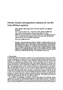
Fig. 1: Gradual HBT.

2. Physical Model For studying electrical behaviour of a gradual heterojunction bipolar transistor such as the one in Fig. 1 Poisson, electron and hole continuity equations have to be solved. In the bulk semiconductor region these equations can be written in a stationary state as [3,4]:

+ div ( ε ∇ψ ) = – q  p – n + N D – N A  

(1)

div ( J n ) = qR

(2)

div ( J p ) = – qR

(3)

where ψ is the electrostatic potential, q is the electron charge, ε is the dielectric constant of the material,- n and p + are the electron and hole densities, N D and N A are the

†[email protected]

Computational Publications, ISSN 1524-2021.

JMSM, Vol. 1, No. 2, Pages 115-120, 1999. doping effective concentrations, and J n and J p are the electron and hole current densities, respectively. The term R represents the volume recombination term, taking into account Schokley-Read-Hall, Auger and band-to-band recombination mechanisms [5]. The carrier currents are controlled by drift-diffusion mechanisms, and may be expressed by: J n = – q µ n n ∇( φ n )

(4)

J p = – q µ p p ∇( φ p )

(5)

where µ n and µ p are the mobilities of electrons and holes, and φ n and φ p are the quasi-Fermi potentials of electrons and holes. Assuming a single parabolic conduction band, the electron density can be expressed as: n = N c F 1 ⁄ 2 ( ηc )

(6)

where N c is the effective density of states in the conduction band, F 1 ⁄ 2 is the Fermi-Dirac integral of order 1/2, and η c is, E fn – E c η c = -------------------kT

(7)

where E fn is the cuasi-Fermi energy of electrons and E c is the conduction band energy. From the aforementioned equations it is easy to obtain the expression (8) for the electron concentration and, using a similar procedure, equation (9) for the hole concentration [6]: q ψ – q φn n = n ien exp  ----------------------  kT 

(8)

qφ p – qψ p = n iep exp  -----------------------  kT 

(9)

N v, ref  q φ p – q ψ ( qχ – qχ ref ) + ( E g – E g, ref ) - – ------------------------------------------------------------------- – ln  ------------η v = -------------------- n i, ref  kT kT

Note that η c and η v depend on the electrostatic potential and the quasi-Fermi potentials. Since these magnitudes are the unknowns in the numerical implementation of the model, an iterative solution process is established in order to guarantee coherent results. The formulation given by (8) and (9) for carrier concentrations is simple and compact. Parameters n ien and n iep may include different phenomena that affect the concentrations at high doping levels: influence of FermiDirac statistics, changes in the energy levels and variations in the effective densities of states. These equations are scaled using the scaling presented in [7]. Next, the finite element method should be applied in order to discretise the scaled equations, thus obtaining a system of nonlinear equations, with range N , where N is the number of nodes of the discretisation [8]. However, the discretisation of J p and J n require particular care. It is necessary to use special schemes such as those developed by ScharfertterGummel [7]. Since we shall have to perform various computations on each one of the elements of the mesh, it is advantageous to transform the elements into a reference element T m . This reference tetrahedron with vertices (0,0,0),(1,0,0),(0,1,0) and (0,0,1) uses the following coordinate transformation: x = ( x 0, x 1, x 2 ), ξ = ( ξ 0, ξ 1, ξ 2 ), x = x ( ξ )

x = x ( ξ ) , B T ( ∆ ψ D ) = diag ( B ( ψ D ( P 0 ) – ψ D ( P 1 ) ), ... ) where B is the Bernoulli function, P 0, P 1, ... be the vertices of the reference element T m , G m the center of gravity of T m , and by x G T = x ( G m ) the image of G m in the element T , we can write: J n, G T = µ n n ien, G T e –t

Nc  qχ – qχ ref   F 1 ⁄ 2 ( η c ) - --------------------- exp  -----------------------n ien = n i, ref  ------------   exp ( η c )   N c, ref  kT

(10)

1 ⁄ 2 ( η v )  F ------------------- exp ( η v )  

116

t

t

(11)

(12)

(15)

–φn D

–ψ D ( P0 )

J e B T ( – ∆ ψ D )J e ∇e

where η c and η v are: N c, ref  q ψ – q φ qχ – qχ ref - – ln  ------------η c = ---------------------n- + ----------------------- n i, ref  kT kT

ψ D ( P0 )

J p, G T = – µ p n iep, G T e –t

Nv   ( qχ – qχ ref ) + ( E g – E g, ref )  - exp  – -----------------------------------------------------------------n iep= n i, ref ------------   N v, ref   kT

(14)

If J e denotes the Jacobian of the map

J e B T ( ∆ ψ D )J e ∇e

where n ien and n iep can be calculated as follows:

(13)

(16)

–φ p D

which correspond to the value of the current density inside an element. The variables marked with subscript D refer to the values of the discretised variable in the nodes of the mesh. Based on these expressions and using the finite elements theory the discretised equations are generated [9,10]. From these equations we obtain the linear systems that we are going to solve with the methods that will be described in the following section.

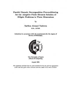
Parallel Domain Decomposition Applied to 3D Simulation of Gradual HBTs interface unknowns, B i represents the equations of internal nodes, C represents the equations of interface nodes, E i represents the subdomain to interface coupling seen from the subdomains and F i represents the interface to subdomain coupling seen from the interface nodes.

External interface nodes

In order to be able to apply these techniques it is necessary to partition the mesh into subdomains for which we have used the program METIS [12]. The same program was subsequently used to relabel the nodes in the subdomains with the purpose of obtaining a more suitable rearrangement. We have used a library of parallel sparse iterative solvers, called PSPARSLIB [13] to solve these linear systems in parallel. A great advantage of this library is that it is optimised for several powerful multicomputers.

Internal nodes

Several domain decomposition techniques were studied with this library, and the best results were obtained with the Additive Schwarz and Schur complement methods. Local interface nodes

3.1. Additive Schwarz

Fig. 2: Nodes in a subdomain.

The additive Schwarz procedure is similar to a block-Jacobi iteration and consists of updating all the new components from the same residual. The basic additive Schwarz iteration would therefore be as follows:

3. Domain Decomposition Solvers Domain decomposition methods refer to a collection of techniques which revolve around the divide and conquer principle. These methods combine ideas from partial differential equations, linear algebra, mathematical analysis and techniques form graph theory [11]. If we consider the problem of solving an equation on a domain Ω partitioned in p subdomains Ω i , then domain decomposition methods attempt to solve the problem on the entire domain by a problem solution on each subdomain Ω i . This means that Ω i 's are such that p

∪i = 1 Ωi

Ω =

(17)

Fig. 2 is an illustration of a subdomain of the physical domain. Each node belonging to a subdomain is an unknown of the problem. It is important to distinguish between three types of unknowns: internal nodes are those that are coupled only with local nodes, local interface nodes are those coupled with external nodes as well as local nodes and external interface nodes are those nodes in other subdomains which are coupled with local nodes. We label the nodes as subdomains, first the internal nodes and then the interface nodes. As a result, the linear system associated with the problem has the following structure, B1 B2

E 1 x1

f1

E 2 x2

f2

. Bp Ep

. = . xs

. . fs

Fp C

y

g

. F1 F2

1.

Obtain y i, ext

2.

Compute local residual r i = ( b – Ax ) i

3.

Solve A i δ i = r i

4.

Update solution x i = x i + δ i

where y i, ext are the external interface nodes. To solve the linear system A i δ i = r i a standard ILUT preconditioner combined with GMRES for the solver associated with the blocks is used [11]. Some zeros in the original matrix may well become nonzeros during the course of ILUT factorization. The number of the new nonzero elements, which we are going to use, is indicated with the fillin parameter. One factor which can affect convergence is the tolerance used for the inner solver. As accuracy increases, the number of outer steps may decrease. However, since the cost of each inner solver increases, this often offsets any gains made from the reduction in the number of outer steps to achieve convergence. It is interesting to observe that the required communication, as well as the overall structure of the routine, is identical with that of matrix-vector products. 3.2. Schur complement techniques Schur complement techniques refer to methods which only iterate on the interface unknowns, implicitly using internal unknowns as intermediate variables.

(18)

where each x i represents the subvector of unknowns that are interior to subdomain Ω i , y represents the vector of all

Consider the linear system (3) for the subdomain Ω i described as, Bi E i xi F i C i yi

=

fi

(19)

gi

in which B i is assumed to be nonsingular. From the first equation of (19) the unknown x can be expressed as 117

JMSM, Vol. 1, No. 2, Pages 115-120, 1999. –1

xi = Bi ( f i – E i yi )

(20)

Upon substituting this into the second equation of (19), the following reduced system is obtained –1

–1

( C i – F i B i E i )y i = g i – iF B i f i

(21)

Where the matrix S i = C i – F i B –i 1 E i is called the Schur complement matrix associated with the y i variable. If this system can be solved, all the interface variables y will become available, and then the remaining unknowns can be computed using (20). Due to the particular structure of B , it should be observed that any linear system solution with it decouples into p separate systems. The parallelism in this situation arises from this natural decoupling.

parameters are the doping profile and the dimensions in µm of each zone, which are shown in Table 1. The voltage in thermal equilibrium for this device in a cross section (plane x z) of this HBT is shown in Fig. 3, for a mesh with 13856 nodes and 70699 elements. Finally, semilogarithmic graphics for the values of the concentration of holes and of electrons are shown in Fig. 4 a) and Fig. 4 b), respectively, using V C = 0.1 , V B = 0.1 , and V E = 0.0 .

0.6 0.4

4. Results

A CRAY T3E distributed memory multicomputer was used to test this software. This computer is a very powerful and flexible parallel scalable system [16]. It comprises up to 2,048 processors connected by a wide bandwidth bidirectional 3-D torus network. Each cell includes a Dec Alpha 21164 microprocessor, local memory and control logic. The capacity of local memory can range from 64 Mbytes to 2 Gbytes.

Voltage

0.2

In order to reduce the simulation time, the program was developed for distributed-memory multicomputers using the MIMD strategy (Multiple Instruction-Multiple Data) under the SPMD paradigm (Simple Program-Multiple Data) [14]. It was implemented using the MPI (Message Passing Interface) message passing standard library [15]. The main advantage of using this library is that it is presently implemented in many computers, which guarantees the portability of the code [16,17].

3

0 2

0.2 1

0.4 0

0.6 1

0.8 1.4

1.2

2

1

0.8

0.6

0.4

0.2

X(um)

3

0

Z(um)

Fig. 3: Voltage in thermal equilibrium. Table 1: Doping profile of gradual HBT. –3

N eff ( cm ) ∆X

∆Y

∆Z

0.5

1.0

0.2

5.0 1017

0.5

1.0

0.1

B(p-GaAs)

5.0 1019

1.5

3.0

0.12

C(n-GaAs)

1.0

1017

1.5

3.0

0.5

SC(n-GaAs)

2.0 1018

3.0

6.0

0.3

1017

Gradded E (n-AlxGa1-xAs) x:0.3 to 0.0

E(n-Al0.3Ga0.7As)

We have analyzed a gradual HBT device such as the one in Fig. 1. It has four zones: the sub-collector (SC), the collector (C), the base (B), and the emitter (E). Some of the main

5.0

20

20

a)

3

15 2

p

10

b)

15 3

n10 2

1

5

1

5

0

0

0

5 1.4

1

1

0

1.2

1

1.4

2

0.8

0.6

Z(micras)

0.4

X(micras) 0.2

0

1.2

1

2 0.8

0.6

3

0.4

0.2

0

3

X(micras)

Z(micras)

Fig. 4: a) Concentration of holes. b) Concentration of electrons.

4.1. Poisson's equation All preconditioners converge for this equation, however there 118

are significant differences in execution time. This simulator takes several minutes to obtain one Gummel iteration, during this iteration the Poisson and electron and hole continuity

Parallel Domain Decomposition Applied to 3D Simulation of Gradual HBTs equations are solved using the Newton method, as it needs to solve several linear systems.

55

Additive Schwarz FGMRES Schur compl. iter. ILU Schur compl. iter.

50 45

We have used a mesh with 24564 nodes and 130402 elements to compare the three solvers. Fig. 6 shows the execution time for Additive Schwarz and others based on Schur complement techniques. For the latter case the Schur Complement matrix is solved by using two different preconditioners, FGMRES [18] and ILU [19]. The best results were obtained using Schur combined with ILU preconditioner, because it has the least number of iterations, as is shown in Table 2.

2.5

Lfill=10 Lfill=20 Lfill=40

a)

Time (sec)

2

1.5

1

0.5

0 2

3

4

1.1

5 6 N. of processors

7

8

Dim. Krylov=15 Dim. Krylov=30 Dim. Krylov=40

1

Time (sec)

30 25 20 15 10 5 0 2

3

4


7

8

Fig. 6: Time of execution for several solvers for Poisson equation.

4.2. Continuity equations We have compared the results that were obtained for the systems associated with the continuity equations. For the linear system associated to hole continuity equation it can be seen in Fig. 5 a) that the Additive Schwarz solver is slower in all cases than the one based on Schur complement techniques using ILU. In the former case it can be observed that time decreases as the number of processors is increased, although with the step-up from 6 to 8 processors hardly any variation is observed. With regard to the second method it does not present the uniform behaviour that we had with the previous solver, it being observed that more time is taken with 4 processors than with 2. This happen due to the fact that the distribution of unknows among the subdomains can generate a linear systems that is difficult to solve. In Fig. 7 b) a similar situation for the case of the matrix associated to electron continuity equation can be seen.

In this work we have analysed the systems associated with Poisson, electron and hole continuity equations which are necessary to solve in the development of simulators of semiconductors devices. All the results have been obtained for a gradual AlGaAs/GaAs HBT.

0.8 0.7 0.6 0.5 0.4 0.3 0.2 2

3

4


7

8

Fig. 5: Time of execution to Additive Schwarz for Poisson equation. a) Influence of fill-in parameter (dim. Krylov=15) b) Influence of size of Krylov subspace (fil-in=10). Table 2: Iterations for Additive Schwarz, Schur with FGMRES and Schur with ILU 2 4 6 8

35

5. Summary

0.9

b)

40 Time(sec)

Fig. 5 a) shows the execution time for a one iteration using additive Schwarz preconditioner for different values of the fill-in parameter. In Fig. 5 b) the influence of the size of Krylov subspace for the resolution of only a linear system is shown. For this preconditioner, using low levels of fill-in and a small size of Krylov subspace leads to lower execution time.

Additive Schwarz 465 371 423 628

Schur-FGMRES 808 710 808 1140

Schur-ILU 22 18 23 23

The program was developed for distributed-memory multicomputers using the MIMD strategy under the SPMD paradigm. The code was implemented using the message passing interface library MPI, what guarantees the portability of the code. All the data were measured on a CRAY T3E distributed-memory multicomputer. In order to solve the systems of linear equations we have tested different methods of domain decomposition, which present great advantages as opposed to the classic methods, as regards to speed and memory requirements. These methods are algorithms that are well suited to this type of computer and which, furthermore, are sufficiently precise and powerful to resolve the associated linear systems originating from the simulation of semiconductor devices. Among these methods based on Schur complement techniques deserve special mention, since these are the ones that use the least time in searching for the solution in all cases studied. 119

JMSM, Vol. 1, No. 2, Pages 115-120, 1999. 7

3.5

Additive Schwarz ILU Schur compl. iter.

6

3 2.5

4

b)

3

Time (sec)

Time (sec)

5

a)

Additive Schwarz ILU Schur compl. iter.

2 1.5

2

1

1 0

0.5 2

3

4


7

8

2

3

4


7

8

Fig. 7: Execution time for hole a) and electron b) continuity equations.

Acknowledgments Supported in part by the Ministry of Education and Science (CICYT) of Spain under the project TIC96-1125-C03. We want to thank CIEMAT (Madrid) for providing us access to the Cray T3E multicomputer. The results for Poisson equation was presented at the International Conference on Modeling and Simulation of Microsystems, San Juan, Puerto Rico, April 19-21, 1999

[9] [10] [11] [12]

References [1]

[2]

[3] [4]

[5]

[6]

[7] [8]

120

S. Yamahata, K. Kurishima, H. Ito, and Y. Matsuoka, "Over-220 GHz- f T -and- f max InP/InGaAs doubleheterojunction bipolar transistors with a new hexagonal-shaped emitter,'' Tech. Diag. GaAs IC Symp., pages 163-166, 1995. A.J. García-Loureiro, J.M. López-González, T. F. Pena, and Ll. Prat, "Numerical analysis of abrupt heterojunction bipolar transistors,'' International Journal of Numerical Modelling: Electronic Networks, Devices and Fields, 8, 221-229, 1998. S. Selberherr. Analysis and Simulation of Semiconductor Devices. Springer, 1984. C. M. Snowden. Semiconductor device modelling. Number 5 in IEE Materials and Devices. Peter Peregrinus Ltd., 1988. C.M. Wolfe, N. Holonyak, and G.E. Stillman. Physical Properties of Semiconductors, chapter 8. Ed. Prentice Hall, 1989. J.M. López-González. Contribution to the study of the Heterojunction Bipolar Transistors. PhD thesis, Universidad Politécnica de Cataluña, 1994. (in Spanish). P.A. Markowich, The Stationary Semiconductor Device Equations, Springer-Verlag, 1986. T.F. Pena, J.D. Bruguera, and E.L. Zapata, "Finite element resolution of the 3D stationary semiconductor device equations on multiprocessors,'' J. Integrated Computer-Aided Engineering, 4, 66-77, 1997.

[13]

[14]

[15] [16]

[17]

[18]

[19]

J. Tinsley and Graham F. Carey. Finite Elements. Prentice-Hall, 1983. O.C. Zienkiewicz. The Finite Element Method. McGraw-Hill, 1977. Y. Saad. Iterative Methods for Sparse Linear Systems, PWS Publishing Co., 1996. George Karypis and Vipin Kumar. METIS: A software package for partitioning unstructured graphs, partitioning meshes, and computing fill-reducing orderings of sparse matrices. Univ. of Minnesota, November 1997. Y. Saad, Gen-Ching Lo, and Sergey Kuznetsov. PSPARLIB users manual: A portable library of parallel sparse iterative solvers. Technical report, Univ. of Minnesota, Dept. of Computer Science, 1997. David A. Patterson and John L. Hennessy. Computer Architecture A Quantitative Approach. Morgan Kaufmann, second edition, 1996. University of Tennessee, MPI: A Message-Passing Interface Standard, 1995. S. L. Scott, "Synchronization and communication in the T3E multiprocessor,'' Technical report, Inc. Cray Research, 1996. D. Sitsky, "Implementation of MPI on the Fujitsu AP1000: Technical details,'' Technical report, Dept. of Computer Science, Australian National Y. Saad and M.H. Schultz. GMRES: a generalised minimal residual algorithm for solving nonsymmetric linear systems. SIAM J. Sci. Statist. Comput., 7:856869, 1986. A. Chapman, Y. Saad, and L. Wigton. High order ILU preconditioners for CFD problems. Technical report, Minnesota Supercomputer Institute. Univ. of Minnesota, 1996. Received in Cambridge, MA, USA, 5th August 1999 Paper 1/02769