The elimination algorithm is designed in such a way, that the fill-in that arises ..... P. Hudak and B. F. Goldberg, âDistributed execution of functional programs ...
Parallel graph reduction for divide-and-conquer applications† Part I - program transformations Willem G. Vree Pieter H. Hartel Computer Systems Department, University of Amsterdam Kruislaan 409, 1098 SJ Amsterdam
Abstract A proposal is made to base parallel evaluation of functional programs on graph reduction combined with a form of string reduction that avoids duplication of work. Pure graph reduction poses some rather difficult problems to implement on a parallel reduction machine, but with certain restrictions, parallel evaluation becomes feasible. The restrictions manifest themselves in the class of application programs that may benefit from a speedup due to parallel evaluation. Two transformations are required to obtain a suitable version of such programs for the class of architectures considered. It is conceivable that programming tools can be developed to assist the programmer in applying the transformations, but we have not investigated such possibilities. To demonstrate the viability of the method we present four application programs with a complexity ranging from quick sort to a simulation of the tidal waves in the North sea.
Key words:
divide-and-conquer parallel algorithms parallel graph reduction reduction strategy program annotation program transformation job lifting
1. Introduction Several parallel architectures have been proposed to support the reduction model of computation. These are based on either string reduction1, 2, 3, 4 or on graph reduction.5, 6, 7, 8, 9, 10, 11, 12 It is often claimed, that for most application programs, graph reduction is more efficient than string reduction. This is due to the fact, that computational work may be shared; upon completion of the work, the result may be used by all interested parties. In this part of † This work is supported by the Dutch Ministry of Science and Education, dienst Wetenschapsbeleid
Vree&Hartel
Parallel graph reduction
1
our paper a mixed reduction model based on normal order evaluation is proposed, which shares some of the advantages of both string and graph reduction.
1.1. A storage hierarchy In graph reduction, a program being executed is represented as a connected graph. Therefore, the graph must be kept in a single storage space. Such a storage space can be implemented in a distributed fashion. In order not to reduce the advantages of sharing, the more frequently non-local accesses occur, the more efficiently they must be performed. In its full generality, this brings about some difficult problems, in particular in the area of garbage collection.13 Our basic model of a distributed architecture is that of a communication network, with processing elements at the nodes. Each processing element has its private store. In most implementations of such architectures, the latency of an access to a non-local store is larger by several orders of magnitude than that of a local access. The slow access is usually implemented in software by interprocess communication through a (serial) data-communication network. Fast access to the local stores is based on exactly the same principles, but the implementation details are different. The communication network is usually a fast parallel bus and the interprocess communication occurs between hardware implemented processes of both the memory and the processor. We do not want to dwell on these details but only stress the large difference in speed between local and global access. An implementation should acknowledge this fact by introducing a distinct category of access primitives for global respectively local access. The purpose of parallel reduction is to speed up computation with respect to sequential reduction. This is achieved by steering the evaluation process in such a way, that reducible expressions appear, which are suitable for evaluation by separate processing elements. The criteria for the selection of such redexes are manifold. For example the granularity of the redexes and their storage requirements play a role. The elected redexes are henceforth called jobs. In our proposal, programs are annotated via the use of a special primitive function. This provides the mechanism by which jobs are announced at run time. When invoked, the subgraph that represents a job is isolated from the rest of the graph, and made self contained. The subgraph is transferred to the private store of the processing element, which is given the task of normalising the job. Upon completion, the resulting subgraph is merged with the original graph. The previously mentioned global access primitives are used exclusively to implement the transfer of jobs and results. The local access primitives are used to dereference pointers in subgraphs, create new nodes etc. An important consequence of this evaluation strategy is that application programs must (be made to) exhibit the right kind of locality in space. Otherwise it is inefficient to evaluate jobs in isolation. String reduction provides this locality in a natural way. Therefore we borrow this property by implanting it in a graph reduction system and show that the disadvantages of string reduction can be avoided.
Vree&Hartel
Parallel graph reduction
2
Our attention is devoted mainly to the development of methods by which applications can be made to exhibit locality in space. This has the advantage, that the choice of reduction system can be separated from issues involved with parallelism. In our opinion it does not matter whether a parallel grain is actually evaluated as one reduction step, or as a number of reduction steps. It is far more important that the grain size, the communication cost and the parallel overhead are well balanced. Since the proposed method is not dependent on any particular reduction system, we also benefit from the more practical advantage that our attention is not sidetracked by new developments in the area of fast sequential reduction methods. Since our project was started, three such discoveries were published.14, 15, 16
1.2. Applications Given a particular application, two different methods can be applied to obtain an optimum in the trade-off between the amount of parallelism and the grain size of parallel computations: Data partitioning This technique applies when the grain size of an application is too large and can be reduced to produce more and finer grains. Divide-and-conquer algorithms use this technique and are the subject of study in the remainder of this paper. Data partitioning can be summarised as: F (union (a, b)) → union ((F a) in parallel with (F b)) Data grouping The grouping technique may be applied when the grain size is too small, but an abundant amount of parallelism is available. Several small grains may be combined into one larger grain, as is shown in the following example: ParMap F (1..10) → SeqMap F (1..5) in parallel with SeqMap F (6..10) Although the example strongly resembles the divide-and-conquer strategy, the mechanism is different. The function ParMap is a parallel version of the sequential map (apply to all) function, SeqMap. In the example ParMap distributes each function application (F i), for i ∈ 1. . 10 to a different processor, whereas SeqMap performs five applications of F in one “grain”. Not all applications may benefit from parallel evaluation on our system. In particular, if the efficiency of a program is based on sharing, which is the case with for instance the Hamming problem,17 then we accept that it cannot benefit from parallel evaluation. In the remainder of the paper we will concentrate on the mechanisms and policies involved in creating and performing “jobs”.
Vree&Hartel
Parallel graph reduction
3
2. Job creation A multiprocessor architecture without a global store limits the amount of parallelism in a functional program that can be usefully exploited, because the communication cost to transport an expression from one local store to another will often dwarf the gain that is obtained by the parallel reduction of that expression. For this reason we have decided only to allow parallel reduction of certain expressions that comply with the notion of a job. We assume, that initially a single expression is presented for evaluation. There must be a significant amount of work involved in this main expression. A job is defined as a reducible expression with the following properties (the so called job conditions): 1.
A job is a closed subexpression (i.e. it contains no free variables).
2.
It’s normal form is needed† in the main expression.
3.
For all concurrent jobs, the communication cost to transport a job must be less than the sum of the reduction costs of the other jobs.
Only subexpressions that are jobs can be submitted to another processor in order to be reduced (in parallel to the main expression and other jobs) by a separate reducer process. It is the responsibility of the programmer to ensure that all job conditions are met. Otherwise parallel evaluation may even cause performance degradation. The restriction of parallel reduction to jobs bears the following advantages: •
Data communication can be based on jobs (and their results) as the smallest quantity of data to be transported. Communication overhead is small compared to communication cost, since in our proposal not just a single packet is transported,7, 12 but a complete subgraph.
•
Since a job is a closed subexpression, it can be reduced in a separate address space. As a consequence no global garbage collection is needed.
•
The process reducing a job is not disturbed by other reducing processes trying to access parts of the job, because all other processes also reduce closed expressions. A reducer only communicates if it needs the result (normal form) of a job submitted by the reducer itself.
•
The parallel reduction of a set of jobs starting at the same time is faster than the sequential reduction of these jobs, provided that sufficient processors are available. The problem of achieving a near optimal distribution of jobs over the available processors during run time has to be solved by an additional load balancing mechanism. The calculation of optimal schedules is pursued in part II of this paper.
To prove the last point we need to formalise job condition (3). Suppose there are n jobs with communication cost c i and reduction cost si , i ∈1 . . n, where c i and si are measured in the same time unit. Job condition (3) then † A subexpression
M
is needed in a context C[M] if and only if
M
is reduced to normal form when C[M] is reduced to normal form.
Vree&Hartel
Parallel graph reduction
4
becomes: ∀ ci < i ∈1..n
n
Σ
k=1, k≠i
sk
(1)
What we want to prove is that the longest job (communication included) takes less time than all jobs in sequence (without communication), i.e.: n
(s k + c k ) Σ s k > max k=1 k=1 n
(2) ci + si < i ∈1..n
From (1) it follows that: ∀
n
Σ s k and therefore (2). k=1
The intuitive version of job condition (3), namely ∀ c i < si is not sufficient to proof (2). Counter example: two i ∈1..n
jobs with c 1 < s1 , c 2 < s2 and c 1 > s2 .
2.1. Sharing To illustrate the consequences of the job concept for parallel graph reduction we will consider the graphical representation of expressions and rephrase job condition (1): 1.
The representation of a job is a subgraph (i.e. there are no references to nodes external to the job).
This condition does not allow for two (or more) jobs to share a subgraph. In the illustration of figure (1) graphs A and B share the subgraph C. Therefore, graph A does not qualify as a job because it contains an external pointer to C.
@A
@B
@S @C
Figure 1 : An external pointer
There are several reasons not to extend the definition of a job to support these external pointers: •
Before submitting a job ( B) all sharing nodes (such as S) have to be discovered and flagged. This is necessary because otherwise the process trying to reduce a sharing node ( S) would not know where to find the result ( C). The discovery of sharing nodes is a time consuming process because the whole graph has to be traversed and marked.
Vree&Hartel
5
Parallel graph reduction
•
The amount of work to reduce a shared expression might be small.
•
After the reduction of job B it is not certain that the expression C has also been reduced. This is the case for example if C is not needed in expression B (e.g. B = if “true” then . . . else C). So A might have waited for a result and still have to do the work.
Considering these difficulties we have decided not to support sharing between jobs and to keep jobs completely self contained. This implies that sharing may only occur within a job. In the example of figure (1) it means that before sending away job B the subexpression C is copied, and both jobs A and B will reduce C.
2.2. Duplication of work The performance gain attained by parallel reduction might well be cancelled by the duplication of work inherent to ordinary string reduction, as is shown in the illustration of figure (2).
C F A
D
E
B
Figure 2 : Nested sharing
The job C is reduced twice, once as part of job A and once as part of job B. However, since D and E are contained in C and share F, F is computed twice for C and thus four times for A. The solution is to reduce F first, supply its normal form to D and E and then reduce C etc. A special parallel reduction strategy has been designed (the “sandwich”-strategy) that avoids duplication of work. It is demonstrated with practical examples that divide-and-conquer algorithms can be converted into sandwich programs.
2.3. The sandwich strategy In a system that exploits strict operator parallelism, a simple job administration is all that is necessary. For example, if some reduction sequence encounters the redex (TRIPLUS x y z), the addition can not be performed until all arguments have been normalised (in parallel). Hence there is no need for the job corresponding to argument x to reactivate the addition before jobs y and z have completed or vice versa. In contrast to strict operator parallelism, a general parallel reduction strategy would allow for any subexpression to be treated as a job. Although more flexible, this has the disadvantage that the administration of jobs is more complex. Suppose, that the generation of parallelism is triggered by annotating subexpressions. For the application
Vree&Hartel
6
Parallel graph reduction
cited above there are several possible ways to annotate one or more of the three arguments. Any completely normalised argument will cause the addition to be reactivated, with the chance that no further progress can be made because some of the arguments are still unavailable. The sandwich strategy combines the advantages of the simple job administration required for strict operator parallelism and the possibility to annotate arbitrary subexpressions, at the detriment of some flexibility. A sandwich expression is defined as a needed function application (G x 1 x 2 . . . x n ) with the following restrictions (the sandwich conditions): 1.
The function G is strict† in all argument positions.
2.
Each argument x i of G is a function application (H i ai1 ai2 . . . aik i ) where:
3.
The function H i is strict in all its arguments.
4.
Each expression (H i ai1 ai2 . . . aik i ) satisfies the job conditions.
5.
The expressions H i an aij are in normal form.
Given a sandwich-expression, the sandwich strategy now runs as follows: •
Submit all function applications (H i ai1 ai2 . . . aik i ) as separate jobs to be reduced in parallel.
•
Wait for the results of all submitted jobs and continue with the normal order reduction of G, applied to the results just received.
The sandwich strategy never duplicates work, because when jobs are submitted and copying takes place, all terms in question are in normal form (H i and aij ). Thus only normal forms are copied and these, by definition, do not contain work. The strategy has been named a “sandwich” because it consists of one layer of parallel and applicative evaluation between two layers of normal evaluation. In the framework of the SASL programming language18 a new primitive function has been introduced, which implements the sandwich strategy. The general form of a sandwich application is: sandwich G (H 1 a11 . . . a1k 1 ) . . . (H n a n1 . . . a nk n ) Apart from parallel evaluation, the expression is equivalent to: G (H 1 a11 . . . a1k 1 ) . . . (H n a n1 . . . a nk n ) The sandwich function evaluates the applications (H i ai1 . . . aik i ) in parallel. As soon as the results of these evaluations have become available, normal lazy evaluation resumes.
† A function G with arity n is strict in argument position i if for every possible redex R, R is needed in (G
x 1 . . . x i−1 R x i+1 . . . x n ).
Vree&Hartel
Parallel graph reduction
7
Summarising, we propose to perform graph reduction within a job and string reduction without duplication of work on the parallel job level. The sandwich strategy exploits strict operator parallelism, but allows the programmer to define the operator.
3. Job control The sandwich strategy provides the means to generate an abundant amount of parallelism, since jobs may contain sandwich expressions, which create new jobs etc. There are two points worth noting: •
Since we strive at obtaining best results with divide-and-conquer problems, it may be assumed that creating more jobs implies that the individual jobs become smaller (in terms of computational work), up to a point where job condition (3) no longer applies.
•
For large problems, an uncontrolled expansion of the population of jobs will outgrow even the most powerful architecture.
Some form of “job control” is necessary to prevent the system from being flooded with small jobs. A good control mechanism would not unduly restrain parallelism, because idle processing elements are a waste of resources. In general the control mechanism must be adaptive to the load of the system. In the architecture proposed here, there is no need for an application independent control mechanism, since all divide-and-conquer algorithms provide a “handle” for regulating the generation of jobs. It is sufficient to make the parallel divide phase conditional to the grain size of the potential jobs. A consequence of the relation between the amount of work involved in the individual jobs and their number is, that a mechanism aimed at keeping the grain size large enough will automatically restrain the number of jobs. A threshold on the grain size is necessary and sufficient. In the next sections examples are given of how the grain size of jobs in divide-and-conquer problems can be calculated and controlled at source level via program transformation. In most other proposals, this control is exerted at a lower level,10, 19, 20 which makes it harder to devise good heuristics.
4. Application of the sandwich strategy As a first example of transforming a divide-and-conquer algorithm into a version suitable for parallel evaluation we consider the quick sort algorithm. The principle of our transformation also applies to other divide-and-conquer algorithms, as will be shown by a parallel version of the fast Fourier transform, Wang’s algorithm for solving a sparse system of linear equations and a hydraulical simulation program.
Vree&Hartel
Parallel graph reduction
8
4.1. Quick sort Figure (3) shows the quick sort algorithm in SASL.21 Before proceeding we will briefly introduce the aspects of the SASL programming language that we need here. A function definition in SASL may consist of several equations. For instance in figure (3) there is one definition of QuickSort, with two alternatives selected by pattern matching on the actual argument. If the list to be sorted is empty, which is written as ( ), the empty list is produced as the answer. In the second equation, the formal argument to QuickSort specifies a pattern (a: x), which is matched with the actual argument when QuickSort is applied to a non-empty list. During the pattern match the head and the tail of the actual argument are made accessible as a and x respectively. In the WHERE definition something similar happens. The result of the application Split a x ( ) ( ) must be a list, the head of which is made accessible as m and the tail as n. When applied to a non-empty list, QuickSort selects the head a of the list and supplies this element as the pivot to the function Split. The tail x of the input list is split around the pivot in two sublists m and n. These sublists are subsequently supplied to recursive invocations of QuickSort. The symbol (++) denotes the infix operator that appends the right list argument to the left one. When (: ) is used as an operator in an expression it prepends a new head to a list. In the Split function a conditional is used to collect the list elements with a value lower than the pivot in the accumulating argument m. The remaining list elements are collected in the second accumulating argument n. The arrow (→) connecting a condition and a clause should be read as then. The else clause of the conditional is Split a y m (b: n). QuickSort ( ) = ( ) QuickSort (a: x) = (QuickSort m) + + (a: (QuickSort n)) WHERE m: n = Split a x ( ) ( ) Split a ( ) m n = m: n Split a (b: y) m n = b < a → Split a y (b: m) n Split a y m (b: n) Figure 3 : Sequential quick sort application
To obtain a parallel version of a program, subexpressions that can be evaluated in parallel must be annotated. To achieve this we use angular brackets ( ‹ and › ), which obey the same syntactic rules as the normal parentheses. An expression between matching angular brackets is a job. Figure (4) shows the version of the QuickSort function after annotation with job brackets. The annotation has to be provided by the programmer.
Vree&Hartel
Parallel graph reduction
9
QuickSort ( ) = ( ) QuickSort (a: x) = ‹ QuickSort m › + + (a: ‹ QuickSort n › ) WHERE m: n = Split a x ( ) ( ) Figure 4 : Quick sort annotated by the programmer with job brackets
A program annotated with job brackets can be transformed more or less automatically into a version with sandwich expressions. A formal description of the transformation may be found in chapter 6. In the remainder of this chapter we will introduce the principles of the transformation by means of a series of examples. The transformation requires two steps. The first step, which we call job lifting, recognises expressions between job brackets. Job lifting generates an auxiliary function G that satisfies the sandwich conditions. In figure (5) job lifting has replaced the body of QuickSort by a sandwich expression of G. QuickSort ( ) = ( ) QuickSort (a : x) = sandwich′ G (QuickSort m) (QuickSort n) WHERE G P Q = P + + (a : Q) m : n = Split a x ( ) ( ) Figure 5 : The job lifted version of quick sort
If both applications of QuickSort in figure (5) were to be reduced in parallel, the application ( Split a x ( ) ( )) would be copied and reduced twice. To solve this problem, we introduce a variant sandwich′ of the sandwich primitive, which normalises all the aij (in casu m and n) before jobs are created. This has the effect of normalising the application ( Split a x ( ) ( )) before the creation of the jobs. For the sandwich strategy to be effective, both recursive applications of QuickSort in figure (5) should contain enough work to outweigh their communication cost (job condition 3). This may be achieved by imposing a lower limit on the length of the lists m and n. Figure (6) shows the final version of the QuickSort program, with controlled application of the sandwich strategy as obtained by a second transformation step. We call this step the grain size transformation. The length of the list to be sorted is taken as a measure of the grain size, since the amount of work is O (length 2 log length). The normalisation forced by the variant sandwich′ is no longer necessary. The reason is, that to determine the lengths of the sublists m and n, both will have to be normalised. The comparisons to the Threshold therefore serve a dual purpose: controlling the grain size and forcing normalisation. Although the final version of the quick sort program has a complex appearance, it should be noted that most of the code is generated by two program transformation steps.
Vree&Hartel
Parallel graph reduction
10
Threshold = 100 QuickSort ( ) = ( ) QuickSort (a : x) = length m > Threshold → length n > Threshold → sandwich G (QuickSort m) (QuickSort n) QuickSort m + + (a : QuickSort seq n) length n > Threshold → QuickSort seq m + + (a : QuickSort n) QuickSort seq m + + (a : QuickSort seq n) WHERE G P Q = P + + (a : Q) m : n = Split a x ( ) ( ) ..................................................................................................................................................................................... QuickSort seq ( ) = ( ) QuickSort seq (a : x) = QuickSort seq m + + (a : QuickSort seq n) WHERE m: n = Split a x ( ) ( ) Split a ( ) m n = m: n Split a (b : y) m n = b < a → Split a y (b : m) n Split a y m (b : n) Figure 6 : Final parallel version of the quick sort program.
The cost involved in the control mechanism that is introduced by the grain size transformation has to be weighed against the benefits from parallel evaluation. The optimal value of the Threshold depends on properties of the system configuration. Both issues are pursued in part II of this paper.22
4.2. The fast Fourier transform The fast Fourier transform processor is an early example of parallel computer architecture. Though several different organisations have been proposed for these special purpose processors,23 none of them exploited the divideand-conquer strategy to obtain parallelism, because the divide-and-conquer strategy requires many processors executing the same algorithm and processors used to be an expensive resource. Unlike the quick sort algorithm the fast Fourier transform perfectly divides the data into two equal parts at each recursive invocation. This should allow for an optimal processor utilisation. Using a free mixture of conventional mathematical notation and SASL syntax, the essential part of the program with the job annotation is shown in figure (7).
Vree&Hartel
→
11
Parallel graph reduction
→
fft 1 r d = d →
→
→
fft n r d = ‹ fft halfn halfr u › + + ‹ fft halfn (halfr + 128) v › WHERE halfn = n / 2 halfr = r / 2 → → → u = x+z → → → v = x−z →
→
→
x , y = split d halfn → → z = y * exp (halfr * i * π / 128) Figure 7 : The annotated 512-point fast Fourier transform program
To simplify the presentation, the length of the data-list to be transformed has been fixed to 512 elements, which explains the origin of the constant 128 in the program. Furthermore the result list produced by this program is not in the right order and has to be passed through a reorder function, which is, again for the sake of simplicity, not shown. For a fixed length fast Fourier transform, like the one in figure (7), the reorder function can be replaced by →
a fixed mapping. The function application (split d n) produces a pair of lists of which the first one contains the first →
→
n elements of d and the second one contains the rest of d (again n elements). The function application →
→
( fft 512 0 d) performs a 512-point fast Fourier transform on the list d that contains 512 complex numbers. All arithmetic on the vector variables is assumed to be complex. A vector of complex numbers is represented by a list of pairs, where each pair contains a real and an imaginary part. Since the fft function already requires the length of the list of data as a parameter this information is readily available for the purpose of controlling the grain size. The transformation from the version of the program shown in figure (7) to the final sandwich version with threshold control can be performed according to the guidelines of chapter 6.
4.3. Wang’s algorithm for solving a sparse system of linear equations Many mathematical models of physical reality consist of a set of partial differential equations. An important step in approximating the solution of such a set of equations is to solve a large set of linear equations. The corresponding matrices often appear to be in a tri-diagonal or block tri-diagonal form. Wang has proposed a partitioning algorithm to achieve parallelism in the elimination process of a tri-diagonal system.24 According to Michielse and van der Vorst25 a slightly modified algorithm is well suited for local memory parallel architectures. The basic idea of the algorithm is to divide a tri-diagonal matrix in equally sized blocks and to try elimination of these blocks in parallel. The two edge blocks (top left and bottom right) are extended by a zero column, to obtain the same size as the other blocks. Figure (8) shows how a 12 × 12 matrix can be split into three blocks.
Vree&Hartel
12
Parallel graph reduction
u
u
0
0
0
u
u
u
0
0
0
u
u
u
0
0
0
u
u
u
u
u
u
0
0
0
0
u
u
u
0
0
0
0
u
u
u
0
0
0
0
u
u
u
u
u
u
0
0
0
u
u
u
0
0
0
u
u
u
0
0
0
u
u
0
0
Figure 8 : Partitioning of a tri-diagonal matrix (u ≠ 0)
Each block can now be eliminated in parallel. Figure (9) illustrates the effect of this part of the algorithm on one block (i.c. the centre block of figure 8).
u
u
u
0
0
0
v
v
0
0
f
0
0
u
u
u
0
0
f
0
v
0
f
0
0
0
u
u
u
0
f
0
0
v
f
0
0
0
0
u
u
u
f
0
0
0
v
u
Figure 9 : First elimination in one block
The elimination algorithm is designed in such a way, that the fill-in that arises (shown by the letter f in figure 9) is confined to the first and fifth columns of the partition. The reason for this confinement becomes apparent when two adjacent blocks that have been processed are shown together, like blocks A and B in figure (10).
Vree&Hartel
13
Parallel graph reduction
A:
v
v
0
0
f
0
f
0
v
0
f
0
f
0
0
v
f
0
f
0
0
0
v
u
v
v
0
0
f
0
f
0
v
0
f
0
f
0
0
v
f
0
f
0
0
0
v
u
B:
f
0
0
0
w
0
0
0
f
0
Figure 10 : Elimination at the borders of the blocks
The rightmost column containing the fill-in of matrix A is the same column as the leftmost column of matrix B, which also contains fill-in. When the top row of block B is used to eliminate the right most value (u) at the bottom row of block A, the latter row only contains non-zero values at the row positions where fill-in still has to be eliminated (see the result in figure 10). If the same elimination is performed on all pairs of border rows of adjacent blocks, the resulting bottom rows of all blocks together constitute a tri-diagonal matrix. Figure (11) shows this subsystem for the example matrix and the result of the elimination. This can be achieved either directly with Gauss elimination or if the system is large enough by recursive application of the partitioning algorithm.
0
w
f
0
0
0
x
0
0
0
0
f
w
f
0
0
0
x
0
0
0
0
f
w
0
0
0
0
x
0
Figure 11 : Elimination of the subsystem
After restoring the rows of the solved subsystem into their original positions as bottom rows of each block (see the left matrix in figure 12) it can be observed, that it is possible to eliminate all the fill-in of a block locally, only using the bottom row of the next higher block. This final elimination step is shown in figure (12) and again all blocks can be processed in parallel.
Vree&Hartel
14
Parallel graph reduction
0
...
x
0
0
0
0
v
v
0
0
f
0
1
0
0
0
f
0
v
0
f
0
0
1
0
0
f
0
0
v
f
0
0
0
1
0
f
0
0
0
x
0
0
0
0
1
Figure 12 : Final elimination
The SASL program that implements the algorithm is shown in figure (13). Partition matrix = ParMap SecondElimination matrix2 WHERE matrix2 = SequentialPart matrix1 matrix1 = ParMap FirstElimination matrix ParMap f (a : ( )) = ( f a) : ( ) ParMap f (a : x) = ‹ f a › : ‹ ParMap f x › Figure 13 : Skeleton of Wang’s algorithm in SASL with annotation
The function FirstElimination incorporates the first local block elimination, which is shown in figure (9). The results of this first parallel step are gathered into matrix1 , which is subsequently reduced sequentially to matrix2 by the function SequentialPart. The latter implements the pair-wise border row elimination of figure (10) and the Gauss elimination of bottom rows from figure (11). Finally, the second local block elimination, which is shown in figure (12), is performed by the function SecondElimination. Parallelism is enforced by the function ParMap, which assumes its second argument to be a list. In order for ParMap to yield a correct result, the matrix should be structured as a list of blocks: (block 1 , block 2 , block 3 , . . . , block n ). This list structure does not cause a performance penalty, because it is traversed in a linear sequence by ParMap. The grain-size of the parallel computations of this program is completely determined by the size of the blocks into which the matrix is initially divided. In contrast to the previous examples, there is no need for dynamic grain size control (see also figure 24).
5. An extension of the reduction model to support persistent results The sandwich strategy imposes a restriction on the type of applications that may be alleviated without loosing the advantages of the strategy. For instance during the first phase of the computation in Wang’s algorithm, each job assigned to process a diagonal block of the matrix produces “fill in”, which must be eliminated during the third phase. The values needed for this elimination are calculated in a second phase. The Gauss elimination in that phase
Vree&Hartel
Parallel graph reduction
15
only requires the values of the matrix elements in the bottom rows of the matrix blocks. The remaining matrix elements are returned with the results of the first phase, only to be incorporated in new jobs when the third phase is started. So a large part of the matrix is transported twice: once as result of the first phase and once as part of a job in the third phase. The structure of the computations in the third phase is the same as that of the first phase, hence the matrix blocks will probable arrive at the same reducer as before. It would have been more efficient to keep the blocks in their respective places and connect the jobs generated during phase three to the “persistent” blocks. A mechanism is proposed, by which a subexpression of a result can be marked, with the following interpretation: •
The marked subexpression in a result is replaced by a “remote name” when the result is returned to its creator. Instead of the subexpression, only the remote name is transmitted.
•
After transmission of the result, the marked subexpression is saved, with its remote name, for future use on the current reducer.
•
When a remote name appears in a job, it will be allocated to the reducer that contains the corresponding (marked) subexpression such that they may be combined to form a complete job. The marking is then automatically destroyed.
A remote name is a unique identification of a subexpression. Except that it is generated and destroyed during reduction, a remote name is similar to the names that may be given to expressions in functional programs. A potential job must not contain more than one remote name, since these may be bound to different physical locations. Outside a job a remote name has no meaning. Furthermore, it may never be dispensed with explicitly, since this would leave an otherwise unreachable subexpression behind, which can not be garbage collected.
5.1. The sandwich and own functions The primitive function own generates a remote name and causes its argument to become a marked subexpression; otherwise it has the same semantics as the identity function. It is sufficient to mark just the root of the graph that represents the subexpression. A remote name is recognised by the sandwich function, if it appears as one of the H i or aij in its second argument. The restriction to certain positions has the advantage, that the implementation of the sandwich function does not have to search for remote names throughout the graph that represents its second argument. In the example shown in figure (14) the own function marks the head of the result list, which is returned by the function H. The latter reuses the value of newhead during its next application.
Vree&Hartel
Parallel graph reduction
16
repeat oldhead oldtail 1 = oldhead : oldtail repeat oldhead oldtail n = repeat newhead newtail newn WHERE newn = n − 1 newhead : newtail = sandwich′ G (remote oldhead oldtail newn) remote oldhead oldtail n = n = 1 → newhead : newtail (own newhead) : newtail WHERE newhead : newtail = H oldhead oldtail H a x = (a + 10) : (x + 7) G (a : x) = a : (x + x) Figure 14 : Cooperation of the sandwich and own functions
To clarify the operational semantics of the own and sandwich primitives, a number of reductions will be shown that appear during the evaluation of the application (repeat 0 0 3). There are two processes involved in this reduction sequence. These have been named parent and child. The steps carried out by the child process are shown offset to the right in figure (15). step parent process 1
repeat 0 0 3
2
sandwich′ G (remote 0 0 2)
6
G (“remote name” : 7)
7
repeat “remote name” 14 2
8
sandwich′ G (remote “remote name” 14 1)
step child process
3
remote 0 0 2
4
H0 0
5
(own 10) : 7
9
remote 10 14 1
10 H 10 14 11 G (20 : 21) Figure 15 : The evaluation of (repeat 0 0 3)
The first application of the sandwich′ function (step 2) is a normal sandwich expression. It creates a job, which is evaluated by the child process. The “remote name” is generated by the application of the own function in step 5. It is returned with the result, while the value 10, which it represents is left behind. Via the application of G (step 6),
Vree&Hartel
Parallel graph reduction
17
The remote name is passed to the next invocation of repeat (step 7). The second sandwich application (step 8) generates a new job, which carries the remote name back to the child process, where it is replaced by the subexpression 10. By then, the third parameter to the function remote has the value 1, such that instead of a (new) remote name, the value 20 is returned with the result. The computation is finished when G has produced its result. In the implementation of this mechanism no global name directory is required, because a remote name carries a system wide address of the expression it represents. This address can be used to send a job containing a remote name from anywhere in the system back to the creator of the remote name.
5.2. A parallel hydraulical simulation A functional program that implements a mathematical model of the tides in the North Sea26 has been transformed into a version that will run efficiently on a parallel local memory architecture by the use of the own function in combination with the sandwich strategy. To be able to apply the sandwich function, the original program, which contains cycles, has to be transformed into a program without cycles. Details of this transformation can be found a paper by one of the authors.27 Here only the essential skeleton of the program will be used to clarify the annotations. Without the use of the own function the tidal model would retransmit large matrices on each iteration of its main recursion. Consequently the program would run much less efficient on a parallel local memory architecture. The Wang partition algorithm, presented in section 4.3, only suffers a small loss in efficiency without the own-annotation, due to the fact that the matrix blocks are only retransmitted once during the whole calculation. The physical model of the tides repeatedly updates a matrix that contains approximations of the x-velocity, the yvelocity and the wave height of the water in each point of a spatial grid. In a parallel version of the program the matrix can be split into as many blocks as the degree of parallelism requires. We only present a partitioning of the matrix into two blocks, to concentrate on the annotation issues. Figure (16) shows the main recursion of the program, which is started with two partitions called Left and Right. These partitions will be updated in parallel. main Left Right n = repeat Update1 (Left : (Right : (LeftBorderOf Right))) n repeat f x 0 = GetRemoteData x repeat f x n = repeat f ( f x) (n − 1) Figure 16 : The main recursion of the tidal model
The function Update1 submits the matrices Left and Right to different processors, where the actual updating takes place in parallel. All subsequent recursive invocations of Update1 will only transmit remote names instead of real matrices, due to the application of the own function in the remote processors (see below). Therefore a special
Vree&Hartel
Parallel graph reduction
18
function GetRemoteData is provided, to force the transmission of the actual matrices at the end of the main recursion. Figure (17) presents the function Update1 . The process of the updating itself is split into two phases, after each of which communication of one border of the matrices takes place. The first phase updates the x-velocity in both matrices and is implemented by the functions UpdateXleft and UpdateXright. In the second phase both the yvelocity and the wave height are updated by the functions UpdateYHleft and UpdateYHright. Both update phases are dependent on each other and have to be run in sequential order. The left and right parts of each update phase are executed in parallel. Update1 M = ‹ UpdateYHleft Left 1 › : ‹ UpdateYHright Right 1 BorderOfLeft 1 › WHERE (Left 1 : BorderOfLeft 1 ) : Right 1 = Update2 M Update2 (Left 2 : (Right 2 : BorderOfRight 2 )) = ‹ UpdateXleft Left 2 BorderOfRight 2 › : ‹ UpdateXright Right 2 › Figure 17 : The two phases of the updating with annotations
The illustration of figure (18) shows the desired communication structure of Update1 and Update2 . The dashed arrows represent the transmission of remote names, whereas the solid arrows denote communication of real data.
Vree&Hartel
19
Parallel graph reduction
Update2 Left 2
UpdateXleft
Borders2
Right 2
UpdateXright
Update1 Right 1
own Left
own Right
Left 1 UpdateYHleft
“left” processor
Borders1
UpdateYHright
“right” processor
Figure 18 : Communication structure of the tidal model
When transforming the definitions of Update1 and Update2 to sandwich versions, the normalising variant of the sandwich has to be used, to obtain the correct sequence of both updates. Once the evaluator requires the result of the function Update1 (see figure #fig twophase#), reduction continues with the normalisation of the arguments Left 1 , Right 1 and BorderOfLeft 1 . This normalisation in turn forces the evaluation of Update2 . So Update2 will execute prior to Update1 . The updating of the x-velocities will run in parallel, yielding the normal forms Left 1 , Right 1 and BorderOfLeft 1 , directly followed by the parallel updating of the y-velocities and wave heights. Figure (17) shows the need for the own function to avoid redundant data communication. After completion of UpdateXleft the resulting matrix Left 1 is returned and passed unmodified as an argument to UpdateYHleft. The updating of matrix Right 2 follows the same pattern. Both matrices are received as a result to be immediately retransmitted as an argument to the next updating phase. If the functions UpdateXleft and UpdateYHleft would be evaluated on the same processor, the matrix Left 1 could be retained in this processor and a remote name could be returned instead. The same applies to the matrix Right 1 and the functions UpdateXright and UpdateYHright. The only real data to be returned and retransmitted is the BorderOfLeft 1 , which travels from the “left” processor to the
Vree&Hartel
Parallel graph reduction
20
“right” processor. Figure (19) shows the annotation that is necessary to obtain the desired behaviour: UpdateXleft Left 2 BorderOfRight 2 = (own Left 1 ) : RightBorderOf Left 1 WHERE Left 1 = updateXleft Left 2 BorderOfRight 2 UpdateXright Right 2 = own (updateXright Right 2 ) Figure 19 : Retention of the left matrix
The function UpdateXleft returns a remote name for matrix Left 1 and real data for the border of Left 1 . The actual updating takes place in the function updateXleft (without capital U). UpdateXright just returns a remote name for matrix Right 1 . Both functions retain the actual matrices in the processors they have been assigned to by the sandwich. Because the remote names Left 1 and Right 1 are passed as arguments to respectively UpdateYHleft and UpdateYHright, applications of the latter functions will subsequently be allocated as jobs to the processors where the matrices Left 1 and Right 1 reside. By retaining the matrices a considerable saving of communication cost is achieved. If the size of the matrix is n then without the own function the amount of data to be communicated would have been n × n, whereas now the information to be transmitted is of the order of n. The functions of the second updating phase are similar to those of the first phase. Because the main recursion of figure (16) applies Update1 to its own output, one can see that the results of UpdateYHleft and UpdateYHright are also redirected without any modification into the next iteration of UpdateXleft and UpdateXright. Figure (20) shows the annotation that is necessary to retain the matrices in their respective processors and to return the actual data of the border of Right 1 : UpdateYHleft Left 2 = own (updateYHleft Left 2 ) UpdateYHright Right 2 BorderOfLeft 2 = (own Right 1 ) : (LeftBorderOf Right 1 ) WHERE Right 1 = updateYHright Right 2 BorderOfLeft 2 Figure 20 : Retention of the right matrix
As before, the update functions (without a capital U) in figure (20) perform the actual updating of the matrices. The function to force the transmission of the remote matrices at the end of the main recursion is shown in figure (21):
Vree&Hartel
Parallel graph reduction
21
GetRemoteData (Left : Right) = ‹ I Left › : ‹ I Right › Figure 21 : Retrieval of both matrices
Both Left and Right will always be remote names during the iteration of updates, due to the effect of the own function (see figures 19 and 20). The two jobs in figure (21) will therefore be sent to the processors where Left and Right happen to reside. Upon reception of these jobs the remote names will be deleted and after the evaluation of (I Left) and (I Right) the result (Left and Right) will be returned. No more retention takes place, because the jobs no longer contain the own function. Finally the two matrices are paired to represent the state of the tidal model after n iterations.
6. Formal description of the transformation schemes In the previous sections we have presented several examples of application programs with jobs that are annotated by job brackets. Only in the first example (QuickSort) the proposed job-lifting and grain size transformations were actually carried out, resulting in a parallel version of the application. In this section we present a formal description of the transformations that is sufficiently general to handle all given example programs. To describe the job lifting and grain size transformations it is sufficient to define a set of functions operating on restricted syntactic domains.28 In particular, no knowledge of the expression syntax of SASL is needed. The required domains are listed in figure (22). From the basic domains the abstract syntax shown in the same figure constructs two composed domains: the set of tokens and the set of sequences of tokens. It should be noted that the job brackets are included in the token domain. No higher level syntactic structures need to be recognised in order to describe the transformations. Syntactic variables and their domains: I L O T S
: : : : :
Identifiers Literals Operators Tokens Sequences
Abstract syntax: S ::= T | S T T ::= I | L | O | WHERE | = | ( | ) | → | ; | , Figure 22 : Syntactic domains and abstract syntax of a definition with jobs
Vree&Hartel
22
Parallel graph reduction
The two main transformation functions are JL (job-lifting) and GS (grain size). Four additional functions are used: SQ (sequential), LF (left grain size test), RF (right grain size test) and AF (annotation). The latter three functions are application dependent and should be specified for each application separately. That is why their names are provided with a suffix F, which represents the name of the function being transformed. The function AF decides which of the two sandwich functions to use, either the strict one (sandwich′ ) or the non-strict version (sandwich). The left and right grain size tests (RF and LF ) generate predicates that yield TRUE whenever the grain size of the jobs is above an application dependent threshold. The transformation functions JL, GS and SQ are defined independently of the application by the equations of figure (23). The job lifting function (JL) transforms a given function definition into a version where the two jobs are lifted from a general expression into a single function application. JL also generates a sequential version of the annotated application that will be called when the grain size drops below the threshold. Next the lifted function definition is passed to the grain size transformation (GS), which inserts the grain size tests and the sandwich application. The auxiliary transformation function SQ serves to replace the name of the function being transformed by the unique identifier F seq . Conventions for variables: F T a, g b, c, d, e, f
: : : :
Conventions for constants:
Identifiers G, P, Q Tokens Sequences Sequences without occurrences of WHERE or =
JL [[ F a = b ‹ c › d ‹ e › f WHERE g ]] = SQ [[ F ]] [[ F a = b (c) d (e) f WHERE g ]] GS [[ F a = G (c) (e) WHERE G P Q = b P d Q f g ]]
JL [[ F a = b ‹ c › d ‹ e › f ]] = SQ [[ F ]] [[ F a = b (c) d (e) f ]] GS [[ F a = G (c) (e) WHERE G P Q = b P d Q f ]]
:
Identifiers
Vree&Hartel
23
Parallel graph reduction
GS [[ F a = G (c) (e) WHERE g ]] = F a = LF [[ a ]] [[ g ]] → RF [[ a ]] [[ g ]] → AF G (c) (e) G (c) (SQ [[ F ]] [[ e ]] ) RF [[ a ]] [[ g ]] → G (SQ [[ F ]] [[ c ]] ) (e) G (SQ [[ F ]] [[ c ]] ) (SQ [[ F ]] [[ e ]] ) WHERE g
SQ [[ F ]] [[ F a ]] = F seq SQ [[ F ]] [[ a ]] SQ [[ F ]] [[ T a ]] = T SQ [[ F ]] [[ a ]] SQ [[ F ]] [[ T ]] = T Figure 23 : Equations job lifting and grain size transformation
The transformation schemes JL and GS can deal with a function that contains more than one equation. The variable F matches the function name in the first equation and the variable a matches all tokens until the equals symbol (=) in the equation with the job brackets ( ‹ and › ). Similarly the variable g matches all remaining equations. Figure (24) shows the functions AF , LF and RF to be used for the transformation of the application programs presented in the previous sections. Together with the transformation schemes of figure (23) they generate parallel sandwich versions of the presented application programs. In those cases, where the grain size predicates are identical to the function TRUE, the conditional statements generated by the grain size transformation can be simplified.
QuickSort FFT Wang Wave Update1 Wave Update2 Wave GetRemoteData
LF
RF
AF
length m > Threshold halfn > Threshold TRUE TRUE TRUE TRUE
length n > Threshold halfn > Threshold TRUE TRUE TRUE TRUE
sandwich sandwich′ sandwich′ sandwich′ sandwich′ sandwich′
Figure 24 : The functions AF , LF and RF for all applications
7. Related work In our opinion locality is an important concept in computer architecture. For instance the success of virtual memory is largely based on locality in space exhibited by most programs. The current proposal can be classified as a “locality first” design, which makes it different from most contemporary research in the area. Related work will be
Vree&Hartel
Parallel graph reduction
24
characterised by the importance attached to the phenomenon of locality in space. A “divide-and-conquer” combinator was first introduced by Burton and Sleep.6 The main topics in their paper are network topology and load distribution strategy. A general annotation scheme for the λ-calculus is developed by Burton,29 which is also applicable to for instance Turner’s combinators. The annotations can be used to control transportation cost of parallel tasks. Although the notion of self contained subexpressions is introduced, the paper does not concern itself with problems associated with practical graph reduction. In recent work, McBurney and Sleep20 propose a paradigm that models divide-and-conquer behaviour. Their results are based on experiments with transputers but the paradigm is not used in a functional context. Linear speedups are reported for small programs. The “RediFlow” architecture10 provides a global address space, but locality is supposed to be inherent to the function level granularity. Divide-and-conquer applications are mentioned as one possible source of parallelism. The problems associated with a template copying implementation of β-reduction in an implementation of the λ-calculus form one of the major topics of another paper by Keller.30 The way a closure is implemented brings about some locality. The “serial” combinator8, 31 is introduced as an optimal grain of parallelism in the context of fully lazy, parallel graph reduction. The practicality of the approach is demonstrated using a network of processing elements, each with a local store only. The architecture supports a global address space, in which each processing element is responsible for a portion of the store. Locality is supposed to be maintained by the way tasks are diffused to the processing elements to which references exist. In contrast to this approach, the sandwich strategy and job concept may be viewed as a combination of user annotated strictness and user annotated combinators. In addition we propose a “threshold” mechanism to dynamically control the grain size of parallel computations. The own function is a user annotated optimisation of data transport. The “GRIP” proposal11, 13 avoids the locality issue by using a (high speed) bus as the connection medium between all major system components (processing elements and intelligent storage units). The machine exploits conservative parallel strategies and a “super” combinator32 model of reduction. In the “FLAGSHIP” machine, both dynamic task relocation and local caches are supposed to increase locality of the fine grained packet rewriting on a local memory architecture.12
8. Conclusions In a parallel graph reduction machine, the optimality of grains of computation depends on properties of the application program and the machine architecture. Based on some commonly observed properties of distributed architectures, a class of application programs has been designated, which if transformed and annotated according to our guidelines will benefit from parallel evaluation on these architectures. In principle our method tries to adapt the locality of the applications to that of the architecture by copying expressions. Duplication of work is avoided by
Vree&Hartel
Parallel graph reduction
25
changing the order of the calculations. Suitable grains of parallel evaluation are obtained by grouping certain computations. Program transformations are necessary to obtain sufficiently large grain computations. With realistic applications these transformations require substantial effort. However because of the referential transparency property of functional programs this effort is less than that incurred in general concurrent programming. It is conceivable that programming tools can be developed to assist the programmer in applying the program transformations, but we have not investigated such possibilities. The sandwich evaluation strategy bridges the gap between divide-and-conquer algorithms and distributed architectures. The method developed to apply this strategy is independent of the functional programming language used. The proposed evaluation strategy will fit most normal order graph reduction systems. The practicality of the proposed annotations is demonstrated by transformation of four applications, ranging from the fast Fourier transform to a tidal model, into versions that will run efficiently on parallel machines based on a local memory architecture. The control over the generation of parallelism and the grain size is exerted by the applications, rather than by the system. Heuristics for grain size control are tailor made to the application program and are therefore a guarantee for best results. By choosing adequate values for a “threshold” parameter, the maximum number of jobs may be kept within limits acceptable to the concrete architecture. This topic and the two more practical issues related to the optimal value of the threshold (see at the end of section 4.1) will be pursued in part II of this paper.22
Acknowledgements We gratefully acknowledge the support of the Dutch parallel reduction machine project team, in particular the fruitful discussions with Henk Barendregt. Arthur Veen made valuable comments on draft versions of the paper.
References 1.
W. E. Kluge, “Cooperating reduction machines,” IEEE transactions on computers C-32(11) pp. 1002-1012 (Nov. 1983).
2.
G. A. Mago´, “A network of microprocessors to execute reduction languages -- Part I,” J. computer and information sciences 8(5) pp. 349-385 (Oct. 1979).
3.
G. A. Mago´, “A network of microprocessors to execute reduction languages -- Part II,” J. computer and information sciences 8(6) pp. 435-471 (Dec. 1979).
Vree&Hartel
4.
Parallel graph reduction
26
P. C. Treleaven and R. P. Hopkins, “A recursive computer for VLSI,” Computer architecture news 10(3) pp. 229-238 (Apr. 1982).
5.
M. Amamiya, “A new parallel graph reduction model and its machine architecture,” pp. 1-24 in Programming of future generation computers, ed. K. Fychi and M. Nivat, North Holland, Amsterdam, Tokyo, Japan (Oct. 1986).
6.
F. W. Burton and M. R. Sleep, “Executing functional programs on a virtual tree of processors,” pp. 187-194 in 1st Functional programming languages and computer architecture, ed. Arvind, ACM, New York, Wentworth-by-the-Sea, Portsmouth, New Hampshire (Oct. 1981).
7.
J. Darlington and M. Reeve, “ALICE: {A} multiple-processor reduction machine for the parallel evaluation of applicative languages,” pp. 65-76 in 1st Functional programming languages and computer architecture, ed. Arvind, ACM, New York, Wentworth-by-the-Sea, Portsmouth, New Hampshire (Oct. 1981).
8.
P. Hudak and B. F. Goldberg, “Distributed execution of functional programs using serial combinators,” IEEE transactions on computers C-34(10) pp. 881-891 (Oct. 1985).
9.
R. M. Keller, G. Lindstrom, and S. Patil, “A loosely-coupled applicative multi-processing system,” pp. 613-622 in 48th National computer conf., ed. R. E. Merwin and J. T. Zanca, AFIPS, New York (Jun. 1979).
10.
R. M. Keller and F. C. H. Lin, “Simulated performance of a reduction based multiprocessor,” IEEE computer 17(7) pp. 70-82 (Jul. 1984).
11.
S. L. Peyton Jones, “Using Futurebus in a fifth-generation computer,” Microprocessors and microsystems 10(2) pp. 69-76 (Mar. 1986).
12.
P. Watson and I. Watson, “Evaluation of functional programs on the Flagship machine,” pp. 80-97 in 3rd Functional programming languages and computer architecture, LNCS 274, ed. G. Kahn, Springer-Verlag, Berlin, Portland, Oregon (Sep. 1987).
13.
S. L. Peyton Jones, “Directions in functional programming research,” pp. 220-249 in SERC conf. on distributed computing systems programme, ed. D. A. Duce, Peter Peregrinus, Brighton, England (Sep. 1984).
14.
T. Johnsson, “Efficient compilation of lazy evaluation,” ACM SIGPLAN notices 19(6) pp. 58-69 (Jun. 1984).
15.
T. H. Brus, M. C. J. D. van Eekelen, M. O. van Leer, and M. J. Plasmeijer, “CLEAN: {A} language for functional graph rewriting,” pp. 364-384 in 3rd Functional programming languages and computer architecture, LNCS 274, ed. G. Kahn, Springer-Verlag, Berlin, Portland, Oregon (Sep. 1987).
16.
J. Fairbairn and S. C. Wray, “Tim: {A} simple lazy abstract machine to execute supercombinators,” pp. 34-45 in 3rd Functional programming languages and computer architecture, LNCS 274, ed. G. Kahn, Springer-Verlag, Berlin, Portland, Oregon (Sep. 1987).
Vree&Hartel
17.
Parallel graph reduction
27
D. A. Turner, “Functional programs as executable specifications,” pp. 29-54 in Mathematical logic and programming languages, ed. C. A. R. Hoare and J. C. Shepherdson, Prentice Hall, London, England (Feb. 1984).
18.
D. A. Turner, “A new implementation technique for applicative languages,” Software−practice and experience 9(1) pp. 31-49 (Jan. 1979).
19.
C. A. Ruggiero and J. Sargeant, “Control of parallelism in the Manchester data flow machine,” pp. 1-15 in 3rd Functional programming languages and computer architecture, LNCS 274, ed. G. Kahn, Springer-Verlag, Berlin, Portland, Oregon (Sep. 1987).
20.
D. L. McBurney and M. R. Sleep, “Transputer based experiments with the ZAPP architecture,” pp. 242-259 in 1st Parallel architectures and languages Europe (PARLE), LNCS 258/259, ed. J. W. de Bakker, A. J. Nijman, and P. C. Treleaven, Springer-Verlag, Berlin, Eindhoven, The Netherlands (Jun. 1987).
21.
D. A. Turner, “SASL language manual,” Technical report, Computing Laboratory, Univ. of Kent at Canterbury (Aug. 1979).
22.
P. H. Hartel and W. G. Vree, “Parallel graph reduction for divide-and-conquer applications -- Part II: program performance,” PRM project internal report, Dept. of Comp. Sys, Univ. of Amsterdam (Dec. 1988).
23.
G. D. Bergland, “Fast Fourier transform hardware implementations -- an overview,” IEEE transactions on audio and electro acoustics AU-17 pp. 104-108 (Jun. 1969).
24.
H. H. Wang, “A parallel method for tri-diagonal equations,” ACM transactions on mathematical software 7(2) pp. 170-183 (Jun. 1981).
25.
P. H. Michielse and H. A. van der Vorst, “Data transport in Wang’s partition method,” Internal report, Dept. of Comp. Sci, Technical Univ. Delft (1986).
26.
W. G. Vree, “The grain size of parallel computations in a functional program,” pp. 363-370 in Parallel processing and Applications, ed. E. Chiricozzi and A. d’Amico, Elsevier Science Publishers, L’Aquila, Italy (Sep. 1987).
27.
W. G. Vree, “Parallel graph reduction for communicating sequential processes,” PRM project internal report, Dept. of Comp. Sys, Univ. of Amsterdam (Aug. 1988).
28.
R. D. Tennent, “The denotational semantics of programming languages,” CACM 19(8) pp. 437-453 (Aug. 1976).
29.
F. W. Burton, “Annotations to control parallelism and reduction order in the distributed evaluation of functional programs,” ACM transactions on programming languages and systems 6(2) pp. 159-174 (Apr. 1984).
30.
R. M. Keller, “Distributed graph reduction from first principles,” pp. 1-14 in Implementation of functional languages, ed. L. Augustsson, R. J. M. Hughes, T. Johnsson, and K. Karlsson, Programming Methodology
Vree&Hartel
Parallel graph reduction
28
group report 17, Dept. of Comp. Sci, Chalmers Univ. of Technology, Goteborg, Sweden, Aspenas, Sweden (Feb. 1985). 31.
P. Hudak and B. F. Goldberg, “Serial combinators: ‘‘Optimal’’ grains of parallelism,” pp. 382-399 in 2nd Functional programming languages and computer architecture, LNCS 201, ed. J.-P. Jouannaud, SpringerVerlag, Berlin, Nancy, France (Sep. 1985).
32.
R. J. M. Hughes, “Super combinators -- A new implementation method for applicative languages,” pp. 1-10 in Lisp and functional programming, ACM, New York, Pittsburg, Pennsylvania (Aug. 1982).