UCRL-TR-222763
Parallel H1-based auxiliary space AMG solver for H(curl) problems
Tz. V. Kolev, P. S. Vassilevski July 11, 2006
Disclaimer This document was prepared as an account of work sponsored by an agency of the United States Government. Neither the United States Government nor the University of California nor any of their employees, makes any warranty, express or implied, or assumes any legal liability or responsibility for the accuracy, completeness, or usefulness of any information, apparatus, product, or process disclosed, or represents that its use would not infringe privately owned rights. Reference herein to any specific commercial product, process, or service by trade name, trademark, manufacturer, or otherwise, does not necessarily constitute or imply its endorsement, recommendation, or favoring by the United States Government or the University of California. The views and opinions of authors expressed herein do not necessarily state or reflect those of the United States Government or the University of California, and shall not be used for advertising or product endorsement purposes. This work was performed under the auspices of the U.S. Department of Energy by University of California, Lawrence Livermore National Laboratory under Contract W-7405-Eng-48.
PARALLEL H 1 -BASED AUXILIARY SPACE AMG SOLVER FOR H(curl) PROBLEMS TZANIO V. KOLEV AND PANAYOT S. VASSILEVSKI Abstract. This report describes a parallel implementation of the auxiliary space methods for definite Maxwell problems proposed in [4]. The solver, named AMS, extends our previous study [7]. AMS uses ParCSR sparse matrix storage and the parallel AMG (algebraic multigrid) solver BoomerAMG [1] from the hypre library. It is designed for general unstructured finite element discretizations of (semi)definite H(curl)) problems discretized by N´ed´elec elements. We document the usage of AMS and illustrate its parallel scalability and overall performance.
1. Introduction Based on a proper stable decomposition of the lowest order N´ed´elec (edge) finite element space, Hiptmair and Xu introduced in [4] an auxiliary space preconditioner for H(curl) problems, which in addition to standard smoothing utilizes efficient auxiliary space solvers for related Poisson problems. Their method borrows the main tool from the auxiliary mesh preconditioners in [6] and [3], namely, the interpolation operator Π, which maps vector fields into the the N´ed´elec finite element space V h . Motivated by these developments, we considered several options for constructing unstructured mesh AMG preconditioners for H(curl)-problems and reported the computational results in [7]. The present report describes a parallel implementation of these methods in the hypre library. We are interested in solving the following variational problem stemming from Maxwell’s equations: (1.1)
Find u ∈ V h :
(α curl u, curl v) + (β u, v) = (f , v) ,
for all v ∈ V h .
Here α > 0 and β ≥ 0 are scalar coefficients. We allow β to be zero in part or the whole domain. In either case the resulting matrix is only semidefinite, and for solvability the right-hand side should be chosen to satisfy compatibility conditions. Let A and b be the stiffness matrix and the load vector corresponding to (1.1). Then the resulting linear system of interest reads, (1.2)
Ax = b.
Note that the coefficients α and β are naturally associated with the “stiffness” and “mass” terms of A. Besides A and b, our solution method for (1.2) requires the following additional information: Date: June 12, 2006–beginning; Today is June 30, 2006. 1991 Mathematics Subject Classification. 65F10, 65N20, 65N30. This work was performed under the auspices of the U. S. Department of Energy by the University of California Lawrence Livermore National Laboratory under contract W-7405-Eng-48. 1
2
TZANIO V. KOLEV AND PANAYOT S. VASSILEVSKI
(1) The discrete gradient matrix G representing the edges of the mesh in terms of its vertices. G has as many rows as the number of edges in the mesh, with each row having two nonzero entries: +1 and −1 in the columns corresponding to the vertices composing the edge. The sign is determined based on the orientation of the edge. We require that G includes all (interior and boundary) edges and vertices. (2) The representations of the constant vector fields (1, 0, 0),(0, 1, 0) and (0, 0, 1) in the V h basis, given as three vectors: Gx , Gy , and Gz . Note that since no boundary conditions are imposed on G, we can compute the above vectors ad Gx = Gh x, Gy = Gh y and Gz = Gh z, where x, y, and z are vectors representing the coordinates of the vertices of the mesh. In addition to the above quantities, our solver can utilize the following (optional) information: (3) The Poisson matrices Aα and Aβ , corresponding to assembling of the forms (α∇u, ∇v) + (βu, v) and (β∇u, ∇v) using standard linear finite elements on the same mesh. As discussed in [7], based on the above quantities we proceed with the construction of the following additional objects: • AG – either the matrix G T AG or the Poisson matrix Aβ (if given). • BG – an efficient solver for AG . • Π – the matrix representation of the interpolation operator from vector linear to edge finite elements. • AΠ – either the matrix Π T AΠ or the block-diagonal matrix diag(Aα ) (if given). • B Π – an efficient solver for AΠ . The solution procedure then is a three-level method using smoothing in the original edge space and subspace corrections based on BG and B Π . We can employ a number of options here utilizing various combinations of the smoother and solvers in additive or multiplicative fashion. If β is identically zero one can skip the subspace correction associated with G, in which case the solver is a two-level method. The remainder of the report is organized as follows. The parallel version of the solver, as implemented in the hypre library is described in Section 2. Section 3 contains a set of numerical experiments demonstrating the parallel scalability and overall performance of the method. Finally, we summarize the results in the concluding Section 4. 2. The AMS solver in hypre In this section we discuss the parallel implementation of the H 1 -based auxiliary space method in the hypre library under the name AMS (Auxiliary space Maxwell Solver). AMS can be used either as a solver or as a preconditioner. We concentrate here on the sequence of hypre calls needed to create and use it as a solver. We start with the allocation of the HYPRE_Solver object: HYPRE_Solver solver; HYPRE_AMSCreate(&solver); Next, we set a number of solver parameters. Some of them are optional, while others are necessary in order to perform the solver setup.
PARALLEL AUXILIARY SPACE AMG
3
AMS offers the option to set the space dimension. By default we consider the dimension to be 3. The only other option is 2, and it can be set with the function given below. We note that a 3D solver will still work for a 2D problem, but it will be slower and will require more memory than necessary. HYPRE_AMSSetDimension(solver, dim); The user is required to provide the discrete gradient matrix G. AMS expects a matrix defined on the whole mesh with no boundary edges/nodes excluded. It is essential to not impose any boundary conditions on G. Regardless of which hypre conceptual interface was used to construct G, one can always obtain a ParCSR version of it. This is the expected format in the following function. HYPRE_AMSSetDiscreteGradient(solver, G); In addition to G, we need one additional piece of information in order to construct the solver. The user has the option to choose either the coordinates of the vertices in the mesh or the representations of the constant vector fields in the edge element basis. In both cases three hypre parallel vectors should be provided. For 2D problems, the user can set the third vector to NULL. The corresponding function calls read: HYPRE_AMSSetCoordinateVectors(solver,x,y,z); or HYPRE_AMSSetEdgeConstantVectors(solver, one_zero_zero, zero_one_zero, zero_zero_one); The vectors one_zero_zero, zero_one_zero and zero_zero_one above correspond to the constant vector fields (1, 0, 0), (0, 1, 0) and (0, 0, 1). The remaining solver parameters are optional. For example, the user can choose a different cycle type by calling HYPRE_AMSSetCycleType(solver, cycle_type); /* default value: 1 */ The available cycle types in AMS are: • cycle_type=1: multiplicative solver (01210) • cycle_type=2: additive solver (0 + 1 + 2) • cycle_type=3: multiplicative solver (02120) • cycle_type=4: additive solver (010 + 2) • cycle_type=5: multiplicative solver (0102010) • cycle_type=6: additive solver (1 + 020) • cycle_type=7: multiplicative solver (0201020) • cycle_type=8: additive solver (010 + 020) Here we use the following convention for the three subspace correction methods: 0 refers to smoothing, 1 stands for BoomerAMG based on BG , and 2 refers to a call to BoomerAMG for B Π . The abbreviation xyyz for x, y, z ∈ {0, 1, 2} refers to a multiplicative subspace correction based on solvers x, y, y, and z (in that order). The abbreviation x + y + z stands for an additive subspace correction method based on x, y and z solvers. The additive cycles are meant to be used only when AMS is called as a preconditioner. In our experience the choices cycle_type=1 and cycle_type=5 often produced fastest solution times, while cycle_type=7 resulted in smallest number of iterations.
4
TZANIO V. KOLEV AND PANAYOT S. VASSILEVSKI
Additional solver parameters, as the maximum number of iterations, the convergence tolerance and the output level, can be set with HYPRE_AMSSetMaxIter(solver, maxit); /* default value: 20 */ HYPRE_AMSSetTol(solver, tol); /* default value: 1e-6 */ HYPRE_AMSSetPrintLevel(solver, print); /* default value: 1 */ More advanced parameters, affecting the smoothing and the internal AMG solvers, can be set with the following three functions: HYPRE_AMSSetSmoothingOptions(solver, 2, 1, 1.0, 1.0); HYPRE_AMSSetAlphaAMGOptions(solver, 10, 1, 3, 0.25); HYPRE_AMSSetBetaAMGOptions(solver, 10, 1, 3, 0.25); For (singular) problems where β = 0 in the whole domain, different (in fact simpler) version of the AMS solver is offered. To allow for this simplification, use the following hypre call HYPRE_AMSSetBetaPoissonMatrix(solver, NULL); If β is zero only in parts of the domain, the problem is still singular, but the AMS solver will try to detect this and construct a non-singular preconditioner. Two additional matrices are constructed in the setup of the AMS method—one corresponding to the coefficient α and another corresponding to β. This may lead to prohibitively high memory requirements, and the next two function calls may help to save some memory. For example, if the Poisson matrix with coefficient β (denoted by Abeta) is available then one can avoid one matrix construction by calling HYPRE_AMSSetBetaPoissonMatrix(solver, Abeta); Similarly, if the Poisson matrix with coefficient α is available (denoted by Aalpha) the second matrix construction can also be avoided by calling HYPRE_AMSSetAlphaPoissonMatrix(solver, Aalpha); Note the following regarding these functions: • Both of them change their input. More specifically, the diagonal entries of the input matrix corresponding to eliminated degrees of freedom (due to essential boundary conditions) are penalized. • HYPRE_AMSSetAlphaPoissonMatrix forces the AMS method to use a simpler, but weaker (in terms of convergence) method. With this option, the multiplicative AMS cycle is not guaranteed not converge with the default parameters. The reason for this is the fact the solver is not variationally obtained from the original matrix (it utilizes the auxiliary Poisson–like matrices Abeta and Aalpha). Therefore, it is recommended in this case to use AMS as preconditioner only. After the above calls, the solver is ready to be constructed. The user has to provide the stiffness matrix A (in ParCSR format) and the hypre parallel vectors b and x. (The vectors are actually not used in the current AMS setup.) The setup call reads, HYPRE_AMSSetup(solver, A, b, x); It is important to note the order of the calling sequence. For example, do not call HYPRE_AMSSetup before calling HYPRE_AMSSetDiscreteGradient and one of the functions HYPRE_AMSSetCoordinateVectors or HYPRE_AMSSetEdgeConstantVectors. Once the setup has completed, we can solve the linear system by calling HYPRE_AMSSolve(solver, A, b, x);
PARALLEL AUXILIARY SPACE AMG
5
Finally, the solver can be destroyed with HYPRE_AMSDestroy(&solver); More details can be found in the files ams.h and ams.c located in the parcsr_ls directory of hypre . 3. Numerical experiments In this section we present results from numerical experiments with AMS used as a preconditioner in PCG. We consider two setups: one using the default solver parameters, and one with an alternative set of parameters. The default solver parameters were already described in the preceding section, but for completeness we give here their corresponding sequence of hypre calls (it is assumed that the user has installed the hypre library [5]): #include "parcsr_ls.h" HYPRE_ParCSRMatrix A; HYPRE_ParVector b, x; HYPRE_ParCSRMatrix G; HYPRE_ParVector one_zero_zero, zero_one_zero, zero_zero_one; /* Declare solver and preconditioner objects */ HYPRE_Solver solver, precond; /* Create PCG solver */ HYPRE_ParCSRPCGCreate(MPI_COMM_WORLD, &solver); HYPRE_PCGSetTol(solver, 1e-6); /* convergence tolerance */ /* Create AMS preconditioner */ HYPRE_AMSCreate(&precond); HYPRE_AMSSetMaxIter(precond, 1); /* do exactly one iteration */ HYPRE_AMSSetTol(precond, 0.0); HYPRE_AMSSetPrintLevel(precond, 0); HYPRE_AMSSetDiscreteGradient(precond, G); HYPRE_AMSSetEdgeConstantVectors(precond, one_zero_zero, zero_one_zero, zero_zero_one); if (beta_is_identically_zero) HYPRE_AMSSetBetaPoissonMatrix(precond, NULL); HYPRE_AMSSetCycleType(precond, 1); HYPRE_AMSSetSmoothingOptions(precond, 2, 1, 1.0, 1.0); HYPRE_AMSSetAlphaAMGOptions(precond, 10, 1, 3, 0.25); HYPRE_AMSSetBetaAMGOptions(precond, 10, 1, 3, 0.25); /* Set preconditioner */
6
TZANIO V. KOLEV AND PANAYOT S. VASSILEVSKI
Figure 1. Initial unstructured tetrahedral mesh on the unit cube. HYPRE_PCGSetPrecond(solver, (HYPRE_PtrToSolverFcn) HYPRE_AMSSolve, (HYPRE_PtrToSolverFcn) HYPRE_AMSSetup, precond); /* Setup */ HYPRE_ParCSRPCGSetup(solver, A, b, x); /* Solve */ HYPRE_ParCSRPCGSolve(solver, A, b, x); The alternative set of parameters differs only in the following calls: HYPRE_AMSSetCycleType(precond, 7); HYPRE_AMSSetAlphaAMGOptions(precond, 6, 0, 6, 0.25); HYPRE_AMSSetBetaAMGOptions(precond, 6, 0, 6, 0.25); As seen from above, in both cases the relative tolerance in PCG was 10−6 . The input matrices and vectors were constructed in parallel using the unstructured finite element package aFEM. In our experiments, we tried to keep the problem size per processor approximately the same (while increasing the number of processors), although the resulting load balance varied somewhat with the number of processors. We tested both versions of AMS on problems with constant and variable coefficients and recorded the results using the following notation: • • • •
np denotes the number of processors in the run, N is the total size of the problem, nit is the number of PCG iterations, tsetup , tsolve and t denote the average times (in seconds) needed for setup, solve and time to solution (setup and solve), respectively, on a machine with 2.4GHz Xeon processors.
3.1. Constant coefficients. First we consider a simple constant coefficients problem with α = β = 1. The domain is the unit cube meshed with an unstructured tetrahedral mesh. The initial coarse mesh, before serial or parallel refinement is shown in Figure 1.
PARALLEL AUXILIARY SPACE AMG
np 1 2 4 8 16 32 64 128 256 512 1024 1 2 4 8 16 32 64
7
AMS AMG N nit tsetup tsolve N nit tsetup tsolve default solver parameters 105,877 11 2.5s 4.9s 17,478 13 0.1s 0.3s 184,820 12 3.5s 8.4s 29,059 14 0.2s 0.5s 293,224 13 2.9s 6.9s 43,881 15 0.1s 0.4s 697,618 14 4.2s 9.7s 110,745 18 0.2s 0.7s 1,414,371 16 4.6s 11.0s 225,102 18 0.3s 0.8s 2,305,232 16 3.9s 9.7s 337,105 20 0.4s 0.9s 5,040,829 18 5.2s 12.8s 779,539 22 0.5s 1.4s 10,383,148 19 6.5s 15.9s 1,682,661 23 0.8s 1.8s 18,280,864 21 7.3s 17.0s 2,642,337 25 1.1s 2.1s 38,367,625 23 9.0s 22.0s 5,845,443 28 1.7s 2.8s 78,909,936 25 17.9s 33.2s 12,923,121 30 4.0s 4.8s alternative solver parameters 105,877 4 5.5s 8.8s 17,478 6 0.4s 0.4s 184,820 4 9.8s 13.5s 29,059 7 0.7s 0.7s 293,224 4 10.5s 10.8s 43,881 7 1.2s 0.8s 697,618 5 21.2s 18.3s 110,745 7 2.1s 1.1s 1,414,371 5 38.0s 20.5s 225,102 7 3.9s 1.3s 2,305,232 5 53.8s 19.4s 337,105 8 7.3s 1.9s 5,040,829 6 79.3s 25.3s 779,539 8 10.7s 2.5s
Table 1. Numerical results for the problem with constant coefficients (α = β = 1) on a cube.
To better assess the quality of the method, we compare the AMS preconditioner with the BoomerAMG preconditioner in hypre applied to a Laplace problem discretized with linear finite elements on the same mesh. The results listed in Table 1 show that the behavior of AMS is qualitatively similar to that of BoomerAMG. This trend, observed in all our experiments, is to be expected since BoomerAMG is used in the auxiliary space solves of the AMS solver. With the default parameters, the number of AMS iterations increases slightly, but the total run time grows slowly and remains less than a minute. The alternative set of solver parameters gives constant number of iterations, but the setup time increases (almost linearly) with the number of processors. The differences between the two sets of parameters are further investigated in Table 2, where we see that the default parameters result in bounded operator complexities for the two internal AMG methods, whereas the alternative parameters lead to high operator complexities. For the definition of grid and operator complexities, and their influence on AMG performance, we refer to [1]. The scalability of the AMS preconditioner is clearly demonstrated in Figure 2, where we compare it with a diagonally scaled PCG solver. We only include results for up to 256 processors, since on 512 processors (around 38M unknowns) the diagonally scaled PCG did not converge in 100, 000 iterations.
8
TZANIO V. KOLEV AND PANAYOT S. VASSILEVSKI
np 1 2 4 8 16 32 64 128 256 512 1024 1 2 4 8 16 32 64
N nit tsetup tsolve gridG opG gridΠ default solver parameters 105,877 11 2.5s 4.9s 1.04 1.08 1.05 184,820 12 3.5s 8.4s 1.04 1.08 1.05 293,224 13 2.9s 6.9s 1.04 1.08 1.05 697,618 14 4.2s 9.7s 1.04 1.09 1.05 1,414,371 16 4.6s 11.0s 1.04 1.10 1.06 2,305,232 16 3.9s 9.7s 1.05 1.11 1.06 5,040,829 18 5.2s 12.8s 1.04 1.08 1.04 10,383,148 19 6.5s 15.9s 1.05 1.12 1.06 18,280,864 21 7.3s 17.0s 1.06 1.13 1.07 38,367,625 23 8.7s 20.6s 1.04 1.09 1.04 78,909,936 25 17.9s 33.2s 1.05 1.12 1.06 alternative solver parameters 105,877 4 5.5s 8.8s 1.79 4.70 1.79 184,820 4 9.8s 13.5s 1.80 4.86 1.83 293,224 4 10.5s 10.8s 1.83 5.77 1.77 697,618 5 21.2s 18.3s 1.89 6.67 1.82 1,414,371 5 38.0s 20.5s 1.92 7.31 1.91 2,305,232 5 53.8s 19.4s 1.97 8.53 1.89 5,040,829 6 79.3s 25.3s 1.80 7.35 1.75
opΠ 1.10 1.10 1.10 1.10 1.12 1.13 1.10 1.15 1.16 1.10 1.17 4.45 4.96 4.83 5.94 6.82 6.80 6.44
5
690 660 630 600 570 540 510 480 450 420 390 360 330 300 270 240 210 180 150 120 90 60 30
10
AMS−PCG DS−PCG
AMS−PCG DS−PCG
4
Number of iterations
Time to solution (seconds)
Table 2. Grid and operator complexities for the subspace solvers in the problem from Table 1.
10
3
10
2
10
1
1
2
4 8 16 32 64 Number of processors
128 256
10
1
2
4 8 16 32 64 Number of processors
128 256
Figure 2. Time to solution (left) and number of iterations (right) for the constant coefficients problem on a cube: AMS versus Jacobi preconditioners. 3.2. Variable coefficients. Next we consider a problem where α and β have different values in two regions of the domain. The geometry and the results with the two sets
PARALLEL AUXILIARY SPACE AMG
9
of parameters are presented in Tables 3–4. Note that this particular test problem was reported to be problematic for geometric multigrid in [2].
np
N
1 83,278 2 161,056 4 296,032 8 622,030 16 1,249,272 32 2,330,816 64 4,810,140 128 9,710,856 256 18,497,920 512 37,864,880 1024 76,343,920 1 83,278 2 161,056 4 296,032 8 622,030 16 1,249,272 32 2,330,816 64 4,810,140 128 9,710,856 256 18,497,920 512 37,864,880 1024 76,343,920
p −8 −4 −2 −1 0 1 2 default solver parameters α = 1, β ∈ {1, 10p } 9 9 9 9 9 9 10 10 10 10 10 10 10 10 11 12 12 12 11 11 12 13 13 13 12 12 12 13 13 13 13 13 13 13 13 15 15 15 15 15 15 15 16 16 16 16 16 15 16 16 16 16 16 16 16 16 19 19 19 19 19 19 19 21 20 20 20 20 20 20 20 20 20 20 20 20 20 β = 1, α ∈ {1, 10p } 10 10 11 10 9 11 12 10 10 11 10 10 11 12 11 11 13 12 11 13 14 13 13 15 14 12 14 16 13 13 14 14 13 14 15 14 15 16 16 15 17 17 16 17 18 17 16 18 19 14 17 17 17 16 18 18 17 19 20 20 19 21 21 19 20 22 22 20 23 24 17 20 21 21 20 22 23
t 4
8
11 11 13 15 15 16 18 17 21 23 21
11 11 13 14 14 15 17 17 20 22 21
5s 9s 9s 12s 13s 14s 17s 23s 27s 32s 56s
13 12 15 16 16 18 19 18 22 24 22
13 12 15 16 16 18 20 19 22 25 23
6s 10s 11s 14s 15s 16s 20s 26s 29s 36s 76s
Table 3. Number of iterations for the problem on a cube with α and β having different values in the shown regions (cf. [2]).
10
TZANIO V. KOLEV AND PANAYOT S. VASSILEVSKI
We observe that the number of iterations is not very sensitive to the magnitude of the jumps in the coefficients. Again, the default parameters lead to overall fastest solution times. For example, we solved a problem with more than 76 million unknowns and 8 orders of magnitude jumps in the coefficients in less than a minute. In contrast, the alternative set of parameters gives almost constant number of iterations, independent of α, β and the problem size, but its overall run time increases similarly to the previous example. np
1 2 4 8 16 32 64 128 1 2 4 8 16 32 64 128
N
p −8 −4 −2 −1 0 1 2 alternative solver parameters α = 1, β ∈ {1, 10p } 83,278 5 4 4 4 4 4 4 161,056 5 4 4 4 4 4 4 296,032 5 5 5 5 5 4 4 622,030 6 5 5 5 5 5 5 1,249,272 6 5 5 5 5 5 5 2,330,816 6 6 6 6 6 6 6 4,810,140 7 5 5 5 5 5 5 9,710,856 6 6 5 6 6 5 6 β = 1, α ∈ {1, 10p } 83,278 8 7 5 4 4 4 4 161,056 8 8 6 4 4 4 5 296,032 8 8 5 5 5 5 5 622,030 9 8 6 5 5 5 5 1,249,272 9 8 6 5 5 5 6 2,330,816 9 8 6 6 6 6 6 4,810,140 9 9 6 5 5 6 6 9,710,856 9 9 7 6 6 6 6
t 4
8
5 5 5 5 5 6 6 6
5 5 5 5 6 6 6 6
12s 22s 18s 41s 59s 44s 99s 184s
5 5 5 5 6 6 6 6
5 5 5 5 6 6 6 6
10s 20s 18s 36s 52s 45s 80s 164s
Table 4. Results with the alternative solver parameters for the problem from Table 3.
3.3. Singular problems. Finally, we report results on problems where β is identically zero in the domain (Table 5) or in part of it (Table 6). In both cases α = 1. The iteration counts in Table 5 are very similar to those in Table 1. As mentioned earlier, when β = 0 the solver reduces to a two-level method, which results in the smaller setup and solution times compared to Table 1. When β is zero only in part of the domain, we can not use the simpler two-level method, but the results shown in Table 6 are still very good and comparable with the previous experiments. 4. Conclusion The AMS preconditioner in hypre is a scalable solver for definite (and semidefinite) Maxwell problems discretized with the lowest order edge finite elements. It requires some
PARALLEL AUXILIARY SPACE AMG
np 1 2 4 8 16 32 64 128 256 512 1024 1 2 4 8 16 32 64
11
AMS AMG N nit tsetup tsolve N nit tsetup tsolve default solver parameters 105,877 11 2.0s 3.7s 17,478 13 0.1s 0.3s 184,820 12 2.8s 6.1s 29,059 14 0.2s 0.5s 293,224 13 2.3s 5.1s 43,881 15 0.1s 0.4s 697,618 15 3.3s 7.3s 110,745 18 0.2s 0.7s 1,414,371 16 3.8s 7.9s 225,102 18 0.3s 0.8s 2,305,232 17 3.3s 7.0s 337,105 20 0.4s 0.9s 5,040,829 19 4.5s 9.2s 779,539 22 0.5s 1.4s 10,383,148 20 5.4s 11.1s 1,682,661 23 0.8s 1.8s 18,280,864 23 5.9s 13.1s 2,642,337 25 1.1s 2.1s 38,367,625 24 10.4s 14.9s 5,845,443 28 1.7s 2.8s 78,909,936 26 10.8s 21.6s 12,923,121 30 4.0s 4.8s alternative solver parameters 105,877 5 4.8s 4.8s 17,478 6 0.4s 0.4s 184,820 6 8.4s 8.7s 29,059 7 0.7s 0.7s 293,224 7 9.1s 7.7s 43,881 7 1.2s 0.8s 697,618 6 18.4s 9.7s 110,745 7 2.1s 1.1s 1,414,371 7 33.4s 12.4s 225,102 7 3.9s 1.3s 2,305,232 8 46.1s 12.5s 337,105 8 7.3s 1.9s 5,040,829 7 70.3s 13.1s 779,539 8 10.7s 2.5s
Table 5. Numerical results for the singular problem on a cube with α = 1 and β = 0. The geometry is the same as in Figure 1.
additional user input: the discrete gradient matrix and the coordinates of the vertices, but it can handle both variable coefficients and singular problems with zero conductivity. In fact, our experiments demonstrate that the performance of AMS on such problems is very similar to that on problems with α = β = 1. The general conclusion from the numerical results is that with its default parameters, AMS can be quite scalable on hundreds of processors. The alternative set of parameters usually needs significantly less (and constant) number of iterations but its total running time is not as scalable. The behavior of AMS on H(curl)) problems is qualitatively similar to that of BoomerAMG on Laplace problems discretized on the same mesh. Thus, any further improvements in BoomerAMG’s parameters, or in AMG in general, will lead to additional improvements in AMS. References [1] V. E. Henson and U. M. Yang, BoomerAMG: A Parallel Algebraic Multigrid Solver and Preconditioner. Applied Numerical Mathematics, 41:155–177, 2002. [2] R. Hiptmair. Multigrid method for Maxwell’s equations. SIAM J. Numer. Anal., 36(1):204–225, 1999.
12
TZANIO V. KOLEV AND PANAYOT S. VASSILEVSKI
np
N nit tsetup tsolve default solver parameters 1 90,496 11 2.0s 4.7s 2 146,055 12 2.7s 7.3s 4 226,984 13 2.3s 6.3s 8 569,578 15 3.7s 9.3s 16 1,100,033 16 3.9s 10.8s 32 1,806,160 17 3.4s 9.1s 64 4,049,344 19 5.1s 12.8s 128 8,123,586 20 6.7s 15.8s 256 14,411,424 22 6.5s 17.2s 512 30,685,829 25 9.5s 22.6s 1024 61,933,284 24 19.5s 44.8s alternative solver parameters 2 146,055 6 7.9s 14.6s 4 226,984 6 8.4s 11.5s 8 569,578 6 28.4s 21.7s 16 1,100,033 7 35.8s 24.0s 32 1,806,160 7 43.5s 18.5s 64 4,049,344 7 91.7s 31.3s Table 6. Initial mesh and numerical results for the problem on a cube with α = 1 and β equal to 1 inside and 0 outside the interior cube.
[3] R. Hiptmair, G. Widmer, and J. Zou, Auxiliary space preconditioning in H(curl), Numerische Mathematik, 103(3):435–459, 2006. [4] R. Hiptmair and J. Xu, Nodal auxiliary space preconditioning in H(curl) and H(div) spaces, Research Report No. 2006-09, Seminar f¨ ur Angewandte Mathematik, Eidgen¨ossische Technische Hochschule, CH-8092 Z¨ urich, Switzerland, May 2006. [5] hypre: High performance preconditioners. http://www.llnl.gov/CASC/hypre/. [6] Tz. V. Kolev, J. E. Pasciak and P. S. Vassilevski, H(curl) auxiliary mesh preconditioning, in preparation [7] Tz. V. Kolev and P. S. Vassilevski, Some experience with a H 1 –based auxiliary space AMG for H(curl)–problems, LLNL Technical Report UCRL-TR-221841. Center for Applied Scientific Computing, Lawrence Livermore National Laboratory, P.O. Box 808, L-561, Livermore, CA 94551, U.S.A. E-mail address:
[email protected],
[email protected]