Parallel Resolution of Alternating-Line Processes by Means of. Pipelining Techniques .... gaussian elimination scheme for the solution along the partitioned ...
Parallel Resolution of Alternating-Line Processes by Means of Pipelining Techniques
D. Espadas, M. Prieto, I.M. Llorente, F. Tirado Departamento de Arquitectura de Computadores y Automática Facultad de Ciencias Físicas Universidad Complutense 28040 Madrid, Spain {despadas, mpmatias, llorente, ptirado}@dacya.ucm.es
y line
The aim of this paper is to present an easy and efficient method to implement alternating-line processes on current parallel computers. First we show how data locality has an important impact on global efficiency, which leads us to the conclusion that one-dimensional decompositions are the most convenient ones for 2D problems. Once this is asserted, a parallel algorithm is presented for the solution of the distributed tridiagonal systems along the partitioned direction. The key idea is to pipeline the simultaneous resolution of many systems of equations, not parallelising each resolution separately. This approach presents good numerical and architectural properties, in terms of memory usage and data locality, and high parallel efficiencies are obtained. For the case of alternating-line processes, the election of the optimal decomposition is studied. The experimental results have been obtained on a Cray T3E.
phases to compute each coordinate separately. For example, the resolution of an elliptic PDE on the 2D structured grid showed in Figure 1 by a full finite difference or volume discretization method implies the solution of a penta-diagonal system with N2 equations. However, ADI discretization implies the resolution of N system of N equations twice: first, lines parallel to x-axis and, second, lines parallel to y-axis. For the case of parallel computers, among the algorithms proposed on the literature [12] [13] [14] [18] [19] [20] [21], we have chosen one based on the pipelining of the systems to be solved, instead of parallelising each resolution separately [15] [16] [17].
y line
Abstract
x line
y line
1. Introduction Alternating-line processes are widely applied in scientific computing: they appear as iterative solvers, like ADI (Alternating Direction Implicit) discretization methods, or as part of more sophisticated methods, like alternating-line robust smoothers in multigrid. ADI methods are widely applied on multidimensional elliptic and parabolic Partial Differential Equations (PDE) in order to avoid the problematic hepta and penta-diagonal systems of equations coming from the full discretizations of 2D and 3D PDE [1]. ADI reduces the solution of equations in higher dimensions to the solution of multiple tridiagonal systems, the solution is therefore efficiently and easily obtained by fast sequential algorithms, such as gaussian elimination. The main idea is to split each time step (or iteration sweep in the elliptic case) into a number of
x line
x line
Figure 1. For each line in x and y axis there is a tridiagonal system to solve.
Another example of alternating-line process is the smoothing of high frequency components of the error on anisotropic PDEs. Classical multigrid algorithms based on point-wise smoothers do not exhibit good convergence rates when solving anisotropic discrete operators. In these cases, robustness can be achieved using alternating-line relaxation (Jacobi or zebra GaussSeidel) combined with standard coarsening [2]. For any of these algorithms to be effective, it is of great importance that there is an efficient use of memory
resources, because, as is well known, the maximum performance obtainable from current microprocessors is mostly limited by the memory access. The peak performance of the processors has increased by a factor of 4-5 every 3 years, and the memory access time has been reduced by a factor of just 1.5-2 over the same period. Thus, the latency of memory access in terms of processor performance grows by a factor of 2-3 every three years, suggesting the existence of some kind of “memory wall”, responsible that application performance was entirely dominated by memory access time [3] [4]. The common technique to bridge this gap and hide the problem is by using a hierarchical memory structure with large and fast cache memories close to the processor. As a result, the memory structure should have strong influence on the design and development of a code, and the programs must exhibit spatial and temporal locality to make efficient use of the cache memory and so keep the processor busy. To make effective use of this memory hierarchy, it is of great importance how data are located in memory, and how they are used and re-used. In parallel computing, this depends on the data partitioning process. This paper is organised as follows. In section 2 we treat the problem of finding the most effective partition for a 2D problem, and its relation with data locality. Once proved that one-dimensional partitions are profitable on this kind of problems, the pipelined gaussian elimination scheme for the solution along the partitioned directions of the alternating-line processes is presented in section 3. In this section the existence of an optimal block size is also discussed. The application of the pipelining approach to the alternating-line problem is studied in section 4, discussing which of the onedimensional decompositions is more suited to it. The paper ends with some conclusions on the subject.
2. Partitioning Regular Domains in 2D applications 2.1. An overview on message sending Message sending between two tasks located on different processors can be divided into three phases: two of them are where the processors interface with the communication system (the send and receive overhead phases), and a network delay phase, where the data is transmitted between the physical processors. Details of what the system does during these phases vary. Typically, however, during the send overhead phase the message is copied into a system-controlled message buffering area, and control information is appended to the message. In the same way, on the receiving process, the message is copied from a system-controlled buffering area into user-controlled memory (receive
overhead is usually larger than send overhead). Due to these local memory copies, as we present in the following section, the communication cost depends not only on the amount of data but also on the spatial data locality of the message.
2.2. The Cray T3E message passing performance The T3E used in this study has 40 DEC Alpha 21164 running at 450 MHz processors. Like the T3D, the T3E contains no board-level cache, but the Alpha 21164 has two levels of caching on-chip: 8 KB first-level instructions and data caches, and a unified, 3-way associative, 96-Kbyte write-back second-level cache. The local memory is distributed across eight banks, and its bandwidth is enhanced by a set of hardware stream buffers. These buffers, which exploit spatial locality alone, can take the place of a large board-level cache, which is designed to exploit both spatial and temporal locality. Each node augments the memory interface of the processor with 640 (512 user and 128 system) external registers (E-registers). They serve as the interface for message sending; packets are transmitted by first assembling them in an aligned block of 8 Eregisters. The processors are connected via a 3D torus with an inter-processor communication bandwidth of 480 Mbytes/sec. Using MPI, however, the effective bandwidth is smaller due to overhead associated with buffering and with deadlock detection. The library message passing mechanism uses the E-registers to implement transfers, directly from memory to memory. Data does not cross the processor bus; it flows from memory into E-registers and out to memory again in the receiving processor. E-registers enhance performance when no locality is available by allowing the on-chip caches to be bypassed. However, if the data to be loaded were in the data cache, then accessing that data via Eregisters would be sub-optimal because the cachebackmap would first have to flush the data from data cache to memory [5] [6] [7]. Figure 2 shows the measured one-way communication bandwidth for different message sizes using MPI. The test program uses all of the 28 processors available in the system for parallel applications. There is always the same sender processor and one receiver processor that varies. The measures demonstrate that there is no difference between close and distant processors in the CRAY T3E.
350
2.4. Linear Decompositions
300 200 150 100 50 0 0
20000000
40000000
60000000
Message Size (bytes)
Figure 2. CRAY T3E message passing performance for contiguous data. The network distance between the processors involved in the communication varies. 140
BW (MB/s)
120 100 80 60 40 20 0
0
5000
10000
15000
20000
25000
30000
The code was written in C, so a two dimensional domain is stored in a row-ordered (x,y)-array. It can be distributed across a 1D mesh of processors following two possible partitionings: x-direction and y-direction. The y-direction partitioning was found to be more efficient (as figure 3 shows, Y-partitioning is around 37% and 35% better than X-partitioning for the 2048element problem using 8 and 16 processors respectively), because the message data exhibits a better spatial locality. X rows boundaries are stride-1 data, but a message using X-partitioning (Y columns) has a stride equal to the number of elements in dimension x. Similar results have been obtained for three-dimensional problems [8]. Although message-passing bandwidth is very important, we should also note that this difference is not only a message passing effect. Y partitioning exploits more efficiently stream buffers because they maximise inner loop iterations
35000
Stride 1 Stride 16 Stride 256
Stride 2 Stride 32 Stride 512
Stride 4 Stride 64 Stride 1024
Stride 8 Stride 128 Stride 2048
Figure 3. CRAY T3E message passing performance using non-contiguous data
Figure 3 shows the impact of the spatial data locality. We use also the simple echo test, but we modify the data locality by means of different strides between successive elements of the message. The stride is the number of double precision data between successive elements of the message, so stride-1 represents contiguous data. For 32 KB messages, stride-1 bandwidth is around 5 times better than stride-16. Beyond Stride-1024 this difference grows, being stride-1 10 times better than stride-2048.
2.3. Partitioning problem For studying the influence of the data spatial locality in the partitionig of a two-dimensional application we have used a typical stencil problem in which groups of neighbouring data elements are combined to calculate a new value. This type of computation is common in image processing, geometric modelling and solving partial differential equations by means of finite difference or finite volume. The simplest approach to parallelizing these kinds of regular applications distributes the data among the processes, and each process runs essentially the same program on its share of the data. For a two dimensional problem there are two possible decompositions: a linear decomposition or a 2D decomposition.
Execution Time (sec)
Message Size (Bytes)
0.4 0.4 0.3 0.3 0.2 0.2 0.1 0.1 0.0
Execution Time (sec)
BW (MB/s)
250
512
1024
2048
0.8 0.7 0.6 0.5 0.4 0.3 0.2 0.1 0.0 512
Proble m Size
X-Partitioning
Y-Partitioning
1024
2048
Proble m Size
X-Partitioning
Y-Partitioning
Figure 4. Different linear partitioning of an stencil application using 16 (on the left) and 8 processors (on the right). The problem size is the number of elements in each dimension for every matrix.
2.5. Optimal Partitioning for 2D regulars domains Over the last decade the partitioning has been focused on reducing communications that are inherent to the parallel program. As is well known, for a ddimensional problem, the communication requirements for a process grow proportionally to the size of the boundaries, while computations grow proportionally to the size of its entire partition. The communication to computation ratio is thus a perimeter-to-surface area ratio in a two-dimensional problem. Moreover, as we have experimentally proved in a previous section, the time required for sending a message from one processor to another is independent of both processor locations. Therefore, there is no sense in talking about physical neighbours, and the mapping of the logical processors over the physical ones is not very important, as far as communication locality is concerned.
Therefore, these ideas suggest a general rule: Higherdimensional decompositions tend to be more efficient than lower-dimensional decompositions [9] [10] [11]. However, as we discussed in the previous section, the communication cost is also a function of the spatial data locality. Therefore, a trade-off between the improvement of the message data locality and the efficient exploitation of the interconnection network exists. The following figures compare the different decompositions for our sample application in the Cray T3E. 1D decomposition is found to be 17 % better than the 2D partitioning for the 2048-element problem using 8 processors. In the 16-processor simulation the differences are lower (only a 3 %) for the same problem size because the local matrices are smaller too. Similar results have been obtained for three-dimensional problems [8].
The pipelined gaussian elimination method sequences the computational tasks between processors, so that each one remains busy almost all the time, except during the idleness phase due to the arrival of the first packet of data from the preceding processor. This delay increases with what we will call block size, that is, the number of systems computed on each pipeline, needed before the next processor can start its calculation. In figure 6 a graphical representation of the computation and communication patterns over the global domain shows how the processors start computing one after another, so filling the pipe and making concurrent computing work. Interchanging of boundaries takes place after the first sweep has ended, i.e., as soon as the necessary data for the following processor to start are available. Note that pipelining is used in both forward and backward sweeps.
Execution Time (sec)
Execution Time (sec)
%ORFN 0.3 0.3 0.2 0.2 0.1 0.1 0.0 512
1024
2048
Problem Size
1D
2D
0.6 0.5 0.4 0.3 0.2 0.1 0.0
3URFHVVRU��
512
1024
2048
Problem Size
1D
2D
Figure 5. Different decompositions for our sample program in the CRAY T3E using 16 (on the left) and 8 processors (on the right). The problem size is the number of cells in each dimension for the finest grid in the multigrid hierarchy.
We should also note that, although we have considered execution time as the only performance metric, a linear decomposition is also more suited to include fast sequential algorithms in the non-partitioned direction. For example, for an alternating-line process, it is possible to apply the classical two-sweep gaussian elimination (also called Thomas’ method) as the sequential algorithm in this direction. Anyway, for the solution of the parallel tridiagonal systems along the partitioned direction a parallel solver is needed.
3. Pipelined Gaussian Elimination The gaussian elimination method for the solution of tridiagonal systems, the optimal one on serial computers, is divided into two stages: forward elimination and backward substitution. On the forward elimination, starting from the upper equation, the lower secondary diagonal is zeroed by means of linear combinations with the upper row. On the backward substitution, independent solutions are found zeroing the upper secondary diagonal [1].
3URFHVVRU��
3URFHVVRU��
3URFHVVRU��
Figure 6. The pipelined gaussian elimination scheme, for 4 processors and 4 blocks. Blocks computed concurrently are equally shadowed.
Although this algorithm has been widely studied, even developing theoretical models in order to study the obtainable efficiencies, and discussing the optimal election of parameters, like the block size [16] [17], these models do not take into account the effect of the cache memory, so not considering the high importance that data locality has on modern parallel computers [8]. Trying to fill this gap between model and reality, our work focuses on experimental results rather than trying to build a model.
3.1. Optimal block size There are two possible one-dimensional domain decompositions for the 2D problem, which are identified as X and Y decompositions, each one determining the data structure of the boundaries that will be interchanged between the processors. In the Y-partition, an artificial frontier is a set of contiguous in memory data (as long as our code was written in C; in Fortran this would be the X partition). In the X-partitioning (if coded in C), the data belonging to the interchangeable boundaries are strided, that is, each element is a fixed number of elements distant in memory from the previous and following elements of the frontier. Combining the partition type and the direction of the calculation sweep, four different computation and communication schemes can be defined, and combined into two for studying the effect of partition in the performance of alternating-line methods. In figure 7 these four schemes are shown, and named as “1” or “2” depending on the kind of boundaries, and as “A” or “B” depending on the sweep direction. ;�GHFRPSRVLWLRQ���6WULGHG�ERXQGDULHV
;
�$
�%