parallelism in biomedical image processing for real time gui ... - Ijates

International Journal of Advanced Technology in Engineering and Science www.ijates.com Volume No.02, Issue No. 06, June 2014 ISSN (online): 2348 – 7550

PARALLELISM IN BIOMEDICAL IMAGE PROCESSING FOR REAL TIME GUI USING MATLAB Sunil Nayak1, Prof. Rakesh Patel 2 1,2

Department of Instrumentation and Control,L. D. College Of Engineering, Ahmedabad(India)

ABSTRACT Bio medical images are quite known for their time consuming phenomenon of processing as it is having more number of pixels. Graphical user Interface has been recent t in trends for processing image such that extracting features in order to make decision. The main problem in GUI is that the quick response is not done due to algorithm is not meeting with the timing constraint with real time. This condition is due to long algorithm is executed in the sequential way. This research article contains the way to reduce the time required to fetch the output b ased on the length of the algorithm. For algorithm edge detection techniques have been taken into consideration and sequential and parallel execution is compared. Keywords: Parallel Image Processing, Real time processing, Parallel Computing. I. INTRODUCTION Edge detection operators are for boundary conditions and can be used in various ways to distinguish the image details in terms of multiple aspects. One has to use various methods of edge detection techniques to identify defect in image. In biomedical ima ge it is most often use of such image processing task. The manner in which the image is repeatedly processed the time required will be long here each edge detection operator is depicted along with mathematical description and time taken by the each operator to execute the function. II. ANALYSIS OF THE BASIC OPERATORS Taylor series analysis depicts that differencing adjacent points provides an estimate of the first order derivative at a point. If the difference is taken between points separated by  x then by Taylor expansion for we obtain:

x

  x   f ( x )   xf ( x )  '

x

2

f ( x)  O (x ) ''

3

2!

…………………………………………….(1)

' By rearrangement, the first order derivative f ( x ) is

Page | 247

International Journal of Advanced Technology in Engineering and Science www.ijates.com Volume No.02, Issue No. 06, June 2014 ISSN (online): 2348 – 7550 f (x)  '

f

x 

x   f (x) x

 O ( x)

…………………………………………………………………(2)

This shows that the difference between adjacent points is an estimate of the first order derivative, with error

O ( x)

.This error depends on the size of the interval  x and on the complexity of the

curve. When  x is large this error can be significant. The error is also large when the high -order derivatives take large values. In practice, the short sampling of image pixels and the reduced high frequency content make this approximation adequate.[1] A change in intensity can be identified by differencing adjacent points. Horizontally adjacent points which are differentiated will detect vertical changes in intensity and is often called a horizontal edge detector by virtue of its action[2]. A horizontal operator will not show up horizontal changes in intensity since the difference is zero. When applied to an image the action of the horizontal edge-detector forms the difference between two horizontally adjacent points, as such detecting the vertical edges. The operators are classified as[5]: 1. First Order Operator 2. Second Order Operator 3. Nonlinear Operator First-order edge detection Many filter masks have been introduced which approximate the first derivative of the image gradient. Three of the most general are shown in below. All three are created as a combination of two kernels: one for the x-derivative and one for the y-derivative. i) Roberts Operator The Roberts cross operator was earliest edge detection operators. It creates basic first order edge detection and uses two templates which difference pixel values in a diagonal manner, as contrary to along the axes’ directions. The two templates are called M+ and M− are given in Fig.1

Fig.1 Roberts operator The simple 2X2 Roberts operators were one of the earliest methods employed to detect edges. The Roberts cross calculates an efficient, simple, 2-D spatial gradient measurement on an image highlighting Page | 248

International Journal of Advanced Technology in Engineering and Science www.ijates.com Volume No.02, Issue No. 06, June 2014 ISSN (online): 2348 – 7550 regions corresponding to edges. The Roberts operator is implemented using two convolution masks, each designed to respond maximally to edges running at 45 to the pixel grid, which return the image xderivative and y-derivative, Gx and Gy respectively. The magnitude |G| and orientation uof the image gradient are thus given by

… … ….. …….. ……………………………………………….…. ………. …… (3)

|G|= G x 2  G y 2

This gives an orientation for a vertical edge which is darker on the left side in the image.

ii) Prewitt edge detection operator Edge detection is akin to differentiation. Since it detects change it is bound to respond to noise ,as well as to step-like changes in image intensity[4]. It is therefore prudent to incorporate averaging within the edge detection process. We can then extend the vertical template, Mx, along three rowand the horizontal template, My, along three columns. These give the Prewitt edge detection operator, which consists of two templates shown in fig. 2.

Fig 2. Prewitt operator The edge magnitude M is the length of the vector and the edge direction  is the angle of the vector M

( x, y) 

M x( x, y)

2

 M y( x, y)

2

……………………………………………………………

….. (4)

Signs ofMxandMycan be used to determine the appropriate quadrant for the edge direction.  ( x , y )  ta n

1

 M y ( x, y)     M x( x, y) 

………… ……………………………………………….…….…… (5)

iii) Sobel edge detection operator

The weight at the central pixels for both Prewitt templates, is doubled, this gives Sobel edge detection operator. Itconsists of two masks to determine the edge in vector form. It performs better than prewitt operator. The coefficients of smoothing within the Sobel operator are shown in Fig 3. are those for a window size of 3.

Page | 249

International Journal of Advanced Technology in Engineering and Science www.ijates.com Volume No.02, Issue No. 06, June 2014 ISSN (online): 2348 – 7550

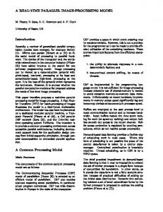
Fig. 3 Sobel Operator iv) Canny edge detection operator

The Canny edge detection operator combined with three main objectives [6]: 1. Optimal detection with no spurious responses 2. Good localization with minimal distance between detected and true edge position 3. Single response to eliminate multiple responses to a single edge. Canny showed that the Gaussian operator was optimal for image smoothing. Recalling that the Gaussian operator by differentiation, for unit vectors Ux= [0,1]and Uy =[1,0]

2 2 ( x y ) 2

g ( x, y, )  e

x 2

( x y

 



2

2

e

….....................................................................................................................................(6)

g ( x, y, )

g (x, y) 

x

2

2

U

2

( x y

)

2

U

x



x



2

2

g ( x, y, )



x

y 2

U

y

…………………………………………..……………………..(7)

)

2

e

U

y

….………………………………………………………………..(8)

A common approximation is, as 1. Use Gaussian smoothing 2. Use the Sobel operator 3. Use non-maximal suppression 4. Threshold with hysteresis to connect edge points

III. METHODOLOGY Four methods are applied sequentially and then four methods were partitioned using two core parallel pools and applied two groups of methods to each core [3].The more mathematical rigorous edge detection technique will be analyzed by time consumed and according to that the data will be portioned. It is obvious that canny and prewitt are quite time consuming by mathematical point of view.

Page | 250

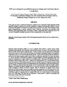
International Journal of Advanced Technology in Engineering and Science www.ijates.com Volume No.02, Issue No. 06, June 2014 ISSN (online): 2348 – 7550 Case: The x ray image of third metacarpal fracture has been taken into investigation for edge detection and GUI has been developed for the same.

Fig 4: GUI for Simultaneous edge detection IV. RESULTS Table 1: Time Calculation for one image: No. 1 2 3 4

Type of Operator Prewitt Sobel Robert Canny

Time Required 0.113993 0.097785 0.101065 0.643522

Sequential time of execution:Elapsed time is 0.956365 seconds. The images are divided in two parts for two cores time required is as follows:

Core1: Prewitt and Sobel Time elapsed is 0.371915 Core 2: Robert and Canny Time elapsed is 0.329901 Page | 251

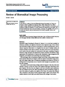
International Journal of Advanced Technology in Engineering and Science www.ijates.com Volume No.02, Issue No. 06, June 2014 ISSN (online): 2348 – 7550 Most significant time taken into the consideration and is of 0.371915 seconds. Efficiency = Es/Ep;[7]……………………………………………………………………………………..(9) Where Es = Sequential time Ep = Parallel time E = 0.956365/0.371915 = 2.57146. Plotting between two algorithm accuracy the time difference is depicted below. The figure5 shows the time difference by time elapsed in second by parallel and sequential algorithm. As number of core is doubled the performance is improved and can be felt.

Ela ps ed ti me

Fig.5: Time difference in sequential and parallel execution for Total execution

V. CONCLUSION The two cores operate efficiently and reduce the time of observer to analyze the results. It is highly desirable to use multicore where using larger datasets as time required manipulating such results is larger in sequential manner.GUI is the tool for real time means no delay between input and output for the process so that the methodology adopted should be used in order to have real time application in MATLAB.As Canny and Prewitt requires more amount of time due to mathematical procedure one should make sure that both should not be allocated to one c ore else contrary condition of timing violation will be there[8]. REFERENCES [1] Dr. S.K.Mahendran, A comparative study on Edge Detection Algorithms for computer aided fracture

detection systems, International Journal of Engineering & Innovative Page | 252

International Journal of Advanced Technology in Engineering and Science www.ijates.com Volume No.02, Issue No. 06, June 2014 ISSN (online): 2348 – 7550 technology , Volume 2.Issue 5,November 2012 [2] Fundamentals of Digital Image Processing: A Practical Approach with Examples in Matlab

by Chris Solomon, Toby

Breckon,

ISBN

978

0

470

84472

4,WileyBlackwell Publication [3] Parallel and Distributed Computing Toolbox Documentation From Mathworks, Inc. [4] Feature Extraction and Image Processing Second

edition by Mark S. Nixon, Alberto

S. Aguado © 2008 Elsevier Ltd [5] Digital Image Processing by BarndJahne ©

Springer-Verlag Berlin Heidelberg 2002

[6] Handbookof Image And Video Processing Editor Al Bovik © 2000 by Academic Press [7] Advanced Computer Architecture And Parallel Processing byHesham El -Rewini and MostafaAbd-El-Barr, ISBN: 0-471-46740-5, Wiley Series On Parallel And Distributed Computing [8] Multi-Core Programming: Increasing Performance through Software Multi-threading by ShameemAkhter& Jason Roberts, ISBN 0-9764832-4-6, INTEL PRESS [9] Textbook of Digital Image Processing By M. Anji Reddy and Y. Hari Shankar© 2006 BS Publication [10] Learning to Program with MATLAB: Building GUI Tools by Craig S. Lent, © 2013 Wiley Global Education

Page | 253