International Journal of Computer Science and Applications, Technomathematics Research Foundation Vol. 12, No. 2, pp. 120 – 143, 2015
GRAPH-BASED SEGMENTATION METHODS FOR PLANAR AND SPATIAL IMAGES Dumitru Dan BURDESCU Computers and information Technology Department Faculty of Automatics, Computers and Electronics, University of Craiova, Bvd. Decebal, Nr. 107, 200440, Craiova, Dolj, Romania
[email protected] Daniel Costin EBANCA Computers and information Technology Department Faculty of Automatics, Computers and Electronics, University of Craiova, Bvd. Decebal, Nr. 107, 200440, Craiova, Dolj, Romania
[email protected] Florin SLABU Computers and information Technology Department Faculty of Automatics, Computers and Electronics, University of Craiova, Bvd. Decebal, Nr. 107, 200440, Craiova, Dolj, Romania
[email protected] The goal of this paper is to present two methods of segmentation on color images based on graphs algorithms. The paper contains two parts. The first part presents Graph-Based Segmentation Method for Planar Images and despite of the majority of the segmentation methods our method does not require any parameter to be chosen in order to produce a better segmentation. A virtual hexagonal structure is created on the pixels of the initial image, and also the initial triangular grid graph having hexagons as vertices. Then the color-based sequence of segmentations and its associated sequence of forests are generated by using the color-based region model and a maximum spanning tree construction method based on a modified form of the Kruskal’s algorithm. The syntactic-based sequence of segmentations and its associated sequence of forests are generated by using the syntactic-based model and a minimum spanning tree construction method based on a modified form of the Boruvka’s algorithm. Finally, color and geometric features are extracted from the determined regions. The second part presents Graph-Based Segmentation Method for Spatial Images. We shall present a unified framework for spatial digital image segmentation and contour extraction that uses a virtual tree-hexagonal structure (prism cells) defined on the set of the input digital image voxels. The advantage of using a virtual tree-hexagonal network superposed over the initial image voxels is that it reduces the execution time because we are using graphs algorithms and their complexities. So, our algorithms are linear on the input the number of the vertices of the spatial input graph. The key to the whole algorithms of spatial segmentation method is the prism cells. This segmentation method contains many other algorithms but only graph-based segmentation algorithm is presented based on the limited space of paper.
Part I. Graph-Based Segmentation Method for Planar Images Abstract 1.1 - The aim in this section is to present a new and efficient graph-based method to detect visual objects from digital color images and to extract their color and geometric features, in order to determine later the contours of the visual objects and to perform syntactic analysis of the determined shapes. The presented method is a general-purpose segmentation method and it produces good results from two different perspectives: 120
Graph-Based Segmentation Methods for Planar and Spatial Images 121 (a) from the perspective of perceptual grouping of regions from the natural images, and also (b) from the perspective of determining regions if the input images contain visual objects. We present a unified framework for planar image segmentation and contour extraction that uses a virtual hexagonal structure defined on the set of the image pixels. This method may be extended for volumetric digital images. The proposed graph-based segmentation method is divided into two different steps: (a) a pre-segmentation step that produces a maximum spanning tree of the connected components of the triangular grid graph constructed on the hexagonal structure of the input image, and (b) the final segmentation step that produces a minimum spanning tree of the connected components, representing the visual objects, by using dynamic weights based on the geometric features of the regions. The pre-segmentation step uses only color information extracted from the input image, whereas the final segmentation step uses both color and geometric and configuration of image regions. Despite of the majority of the segmentation methods our method does not require any parameter to be chosen in order to produce a better segmentation and thus our method it is totally adaptive. Keywords: 1.1 • Algorithm • Graph-based segmentation • Color- based Segmentation • Syntacticbased Segmentation • Visual syntactic features • Dissimilarity
1.
Introduction of Part I
The problem of partitioning images into homogenous regions or semantic entities is a basic problem for identifying relevant objects. Higher-level problems such as object recognition and image indexing can also make use of segmentation results in matching, to address problems such as figure-ground separation and recognition by parts. In both intermediate level and higher-level vision problems, contour detection of objects in real images is a fundamental problem. However the problems of image segmentation and grouping remain great challenges for computer vision. Visual is related to some semantic concepts because certain parts of a scene are preattentively distinctive and have a greater significance than other parts. Objects are defined as visually distinguishable image compounds that can characterize visual properties of corresponding object classes and they have been proposed as an effective middle-level representation of image content. An important approach for object detection is segmentation, and developing an accurate image segmentation technique which partitions image into regions is an important step toward object detection. Unfortunately the goal of the most part of the region detection techniques is to extract a single object in the image. However many real images contain multiple structures, and the most structure may not be unambiguous defined. As a consequence we consider that a segmentation method can detect visual objects from images if it can detect at least the most objects. In this paper, we study the planar segmentation problem in a general framework of image indexing and semantic image processing, where information extracted from detected visual objects, including color features of regions and geometric features of regions and contours will be further used for image indexing and semantic processing. We develop a region-based, computationally efficient, segmentation method that captures both certain perceptually important local and non-local image characteristics. We develop a visual feature-based method which uses a graph constructed on a hexagonal structure containing less than half of the image pixels in order to determine a forest of spanning trees for connected component representing visual objects. Thus the image segmentation is treated as a planar graph partitioning problem. Many approaches aim to create large regions using simple homogeneity criteria based only on color or texture. However,
122 Dumitru Dan BURDESCU, Daniel EBINCA, Florin SLABU
applications for such approaches are limited as they often fail to create meaningful partitions due to either the complexity of the scene or difficult lighting conditions. We determine the segmentation of a color image in two distinct steps: a pre-segmentation step when only color information is used in order to determine an initial segmentation, and a syntactic-based segmentation step when we define a predicate for determining the set of nodes of connected components based both on the color distance and geometric properties of regions. The novelty of our contribution concerns: (a) the virtual hexagonal structure used in the unified framework for image segmentation, (b) the using of maximum spanning trees for determining the set of nodes representing the connected components in the presegmentation step, (c) an adaptive method to determine the thresholds used both in the pre-segmentation and in the segmentation step, and (d) an automatic stopping criterion used in the segmentation step. In addition our segmentation method produces good results from both from the perspective perceptual grouping, and from the perspective of determining regions in the input images. We refer the term of perceptual grouping as a general expectation for a segmentation algorithm to produce perceptually coherent segmentation of regions at a level comparable to humans. 2. Related Works of Part I There are many proposed techniques for color segmentation methods and contour extraction objects. In these methods, the image is modeled as a weighted, undirected graph. Based on number of the edges of the input planar graph G = (V,E) of the colorbased algorithm, and the number of the vertices of input graph we say and prove that the time of segmentation algorithm is linear [14]. In this part we briefly consider some of the related works that are most relevant related to our approach. Usually a pixel or a group of pixels are associated with nodes and edge weights define the dissimilarity between the neighborhood pixels [1]. Most graph-based segmentation methods attempt to search a certain structures in the associated edge weighted graph constructed on the image pixels, such as minimum spanning tree [2], [3] or minimum cut [4], [5]. The major concept used in graph-based segmentation algorithms is the concept of homogeneity of regions. For color segmentation algorithms the homogeneity of regions is color-based, and thus the edge weights are based on color distance. The segmentation criterion is to break the edges with the largest weight, which reflect the low-cost connection between two elements. Other methods [2] and [3] use an adaptive criterion that depends on local properties rather than global ones. In contrast with the simple graph-based methods, cut-criterion methods capture the non-local properties of the image. The methods based on minimum cuts in a graph are designed to minimize the similarity between pixels that are being split [4]. The normalized cut criterion [5] takes into consideration self similarity of regions. An alternative to the graph cut approach is to look for cycles in a graph embedded in the image plane. Other approaches to image segmentation consist of splitting and merging regions according to
Graph-Based Segmentation Methods for Planar and Spatial Images 123
how well each region fulfills some uniformity criterion [6], [7], [8] and [9] and such methods use a measure of uniformity of a region. Graph-based image segmentation techniques generally represent the problem in terms of a graph. The construction principle of this graph is that each node corresponding to a pixel in the image is connected to a fixed number of nearest neighbors measured by color value and the connected neighbors are distributed in four directions [10]. Image segmentation is the process of clustering pixels into image regions corresponding to individual surfaces, objects or natural parts of objects. Image segmentation plays a vital role in image analysis and computer vision applications. Segmentation process should be stopped when region of interest is separated from the input image. Based on the application, region of interest may differ and hence none of the segmentation algorithm satisfies the global applications. Thus segmentation still remains a challenging area for researchers [11]. Our previous works [12], [13] and [14] are related to the works in [2] and [3] in the sense of pair wise comparison of region similarity. In this paper we extend our previous works by adding new steps in the segmentation algorithm that allow us to determine regions closer to the regions. An image processing task contains mainly three important components: acquisition, processing and visualization. After the acquisition stage an image is sampled at each point on a two dimensional grid storing intensity or color information and implicit location information for each sample. The rectangular grid is the most dominant of any grid structure in image processing and conventional acquisition devices acquire square sampled images. The processing stage uses in this case a square lattice model of the input image. An important advantage of using rectangular grid is the fact that the visualization stage uses directly the square pixels of the digitized image. Another two dimensional grid used in the image processing stages is the hexagonal grid [19], [20] and [21]. The hexagonal structured pixel grid is considered to be superior to the rectangular grid system in many respects, including greater angular resolution, and the consistent connectivity [19] and [21]. The algorithms of the processing stage use in this case a hexagonal lattice model of the input image [21]. 3. Constructing a Virtual Hexagonal Structure over an Input Image Because conventional acquisition devices acquire square sampled images, a common approach to acquiring hexagonally sampled images is to convert the input image from a square lattice to a hexagonal lattice, a process known as image re-sampling. We do not use a hexagonal lattice model because of the additional actions involving the double conversion between square and hexagonal pixels. However we intent to use some of the advantages of the hexagonal grid such as uniform connectivity. In this case only one type of neighborhood is possible in the hexagonal grid, the 6-neighbourhood structure, unlike several types as N4 and N8 in the case of square lattice. This implies that there will be less ambiguity in defining boundaries and regions [21]. As a consequence we construct a virtual hexagonal structure over the square pixels of an input image, as presented in Figure 1.1. This virtual hexagonal grid is not a hexagonal lattice because the constructed hexagons are not regular.
124 Dumitru Dan BURDESCU, Daniel EBINCA, Florin SLABU
Let I be an initial image having the dimension w×h (e.g. a matrix having ‘h’ rows and ‘w’ columns of square pixels). In order to construct a hexagonal grid on these pixels we retain an eventually smaller image with h′ = h−(h−1) mod 2, w′ = w−w mod 4. (1.1)
Figure 1.1 Hexagonal structure constructed on the image pixels In the reduced image at most the last line of pixels and at most the last three columns of pixels are lost, assuming that for the initial image h > 3 and w > 4, that is a convenient restriction for input images. Each hexagon from the hexagonal grid contains eight pixels: - six pixels from the frontier and two interior pixels. Because square pixels from an image have integer values as coordinates we select always the left pixel from the two interior pixels to represent with approximation the gravity center of the hexagon, denoted by the pseudo-gravity center. We use a simple scheme of addressing for the hexagons of the hexagonal grid that encodes the location of the pseudo-gravity centers of the hexagons as presented in Figure 1.1. Let w×h the dimension of the initial image verifying the previous restriction (e.g. h mod 2 = 1, w mod 4 = 0, h ≥ 3 and w≥4). Given the coordinates of a pixel ‘p’ from the input image, we use the linear function, ipw,h() =(l −1)w+c, in order to determine an unique index for the pixel. Let ‘ps’ be the sub-sequence of the pixels from the sequence of the pixels of the initial image that correspond to the pseudo-gravity center of hexagons, and ‘hs’ the sequence of hexagons constructed over the pixels of the initial image. For each pixel ‘p’ from the sequence ‘ps’ having the coordinates , the index of the corresponding hexagon from the sequence ‘hs’ is given by the following relation: f hw,h() = [(l−2)w+c−2l]/4+1 (1.2) In this case the following relation holds: f hw,h() = i. (1.3) This states in fact that the scheme of addressing for the hexagons is linear and it has a natural order induced by the sub-sequence of pixels representing the pseudo-gravity center of hexagons.
Graph-Based Segmentation Methods for Planar and Spatial Images 125
Moreover it is easy to verify that the function ‘f h’ defined by the relation (1.2) is bijective. Its inverse function is given by: f h−1w,h(k) = , (1.4) where: l =2+ [4(k−1)]/w if h < w, l = 2+ [4(k−1)]/w +tw if h ≥ w, and h = tw+h′, (1.5) c = 4(k−1)+2l−(l−2)w. (1.6) Relations (1.4), (1.5), and (1.6) allow to uniquely determine the coordinates of the pixel representing the pseudo-gravity center of a hexagon specified by its index (its address). In addition these relations allow us to determine the sequence of coordinates of all eight pixels contained into an hexagon with an address ‘k’: p8(k) = , (1.7) where = f h−1w,h(k) The sub-sequence ‘ps’ of the pixels representing the pseudo-gravity center and the function ‘f h’ defined by the relation (1.2) allow to determine the sequence of the hexagons ‘hs’ that is used by the segmentation and contour detection algorithms. After the processing step the relations (1.4), (1.5), (1.6), and (1.7) allow to update the pixels of the initial image for the visualization step. Each hexagon represents an elementary item and the entire virtual hexagonal structure represents a triangular grid graph, G = (V,E), where each hexagon ‘H’ in this structure has a corresponding vertex v ∈V. The set E of edges is constructed by connecting hexagons that are neighbors in a 6-connected sense. The vertices of this graph correspond to the pseudo-gravity centers of the hexagons from the hexagonal grid and the edges are straight lines connecting the pseudo-gravity centers of the neighboring hexagons, as presented in Figure 1.2.
Figure 1.2 The triangular grid graph constructed on the pseudo-gravity centers of the hexagonal grid There are two main advantages when using hexagons instead of pixels as elementary piece of information:
126 Dumitru Dan BURDESCU, Daniel EBINCA, Florin SLABU
• The amount of memory space associated to the graph vertices is reduced. Denoting by ‘np’ the number of pixels of the initial image, the number of the resulted hexagons is always less than (np/4), and thus the cardinal of both sets V and E is significantly reduced; • The algorithms for determining the visual objects and their contours are much faster and simpler in this case (it is similar of graph algorithms). We associate to each hexagon ‘H’ from V two important attributes representing its dominant color and the coordinates of its pseudo-gravity center, denoted by g(h). The dominant color of a hexagon is denoted by c(h) and it represents the color of the pixel of the hexagon which has the minimum sum of color distance to the other seven pixels. Each hexagon ‘H’ in the hexagonal grid is thus represented by a single point, g(h), having the color c(h). By using the values g(h) and c(h) for each hexagon information related to all pixels from the initial image is taken into consideration by the segmentation algorithm. 4. Planar Segmentation Algorithm Let V = {h1, . . . ,h|V|} be the set of hexagons constructed on the input image pixels as presented in previous section, and G = (V,E) be the undirected grid-graph, with E containing pairs of hexagons that are neighbors in a 6-connected sense. The weight of each edge e = (hi,hj) is denoted by w(e), or similarly by w(hi,hj), and it represents the dissimilarity between neighboring elements ‘hi’ and ‘hj’ in a some feature space. Components of an image represent compact regions containing pixels with similar properties. Thus the set V of vertices of the graph G is partitioned into disjoint sets, each subset representing a distinct visual object of the initial image. As in other graph-based approaches [2] we use the notion of segmentation of the set V. A segmentation, S, of V is a partition of V such that each component C ∈ S corresponds to a connected component in a spanning sub-graph GS = (V,ES) of G, with ES ⊆E. The set of edges E −ES that are eliminated connect vertices from distinct components. The common boundary between two connected components C′,C′′ ∈ S represents the set of edges connecting vertices from the two components: cb(C′,C′′) = {(hi,hj) ∈ E | hi ∈ C′, hj ∈ C′′} (1.8) The set of edges E−ES represents the boundary between all components in S. This set is denoted by bound(S) and it is defined as follows: bound(S)= ∪C′,C′′∈ S cb(C′,C′′) (1.9) In order to simplify notations throughout the paper we use Ci to denote the component of a segmentation S that contains the vertex hi ∈V. We use the notions of segmentation too fine and too coarse as defined in [2] that attempt to formalize the human perception of visual objects from an image. A segmentation S is too fine if there is some pair of components C′,C′′ ∈ S for which there is no evidence for a boundary between them. S is too coarse when there is proper refinement of S that is not too fine. The key element in this definition is the evidence for a boundary between two
Graph-Based Segmentation Methods for Planar and Spatial Images 127
components. The goal of a segmentation method is to determine a proper segmentation, which represent salient objects from an image. Definition 1.1 Let G = (V,E) be the undirected graph constructed on the hexagonal structure of an planar image, with V = {h1, . . . ,h|V|}. A proper segmentation of V, is a partition S of V such that there exists a sequence of segmentations of V for which: • S = S f is the final segmentation and Si is the initial segmentation, • S j is a proper refinement of S j+1 (i.e., S j ⊂ S j+1) for each j = i, . . . , f −1, • segmentation S j is too fine, for each j = i, . . . , f −1, • any segmentation Sl such that S f ⊂ Sl , is too coarse, • segmentation S f is neither too coarse nor too fine. In the above definition Sa is a refinement of Sb in the sense of partitions, i.e. every set in Sa is a subset of one of the sets in Sb. We say that Sa is a proper refinement of Sb if Sa is a refinement of Sb and Sa ≠Sb. In the case of a proper refinement, Sa is obtained by splitting one or more components from Sb, or similarly, Sb is obtained by merging one or more components from Sa. Let C′,C′′ ∈ Sa be two components obtained by splitting a component C ∈ Sb. In this case C′ and C′′ have a common boundary, cb(C′,C′′) ≠Ø. Our segmentation algorithm starts with the most refined segmentation, S0 = {{h1}, . . . ,{h|V|}} and it constructs a sequence of segmentations until a proper segmentation is achieved. Each segmentation S j is obtained from the segmentation S j−1 by merging two or more connected components for there is no evidence for a boundary between them. For each component of a segmentation a spanning tree is constructed and thus for each segmentation we use an associated spanning forest. The evidence for a boundary between two components is determined taking into consideration some features in some model of the image. When starting, for a certain number of segmentations the only considered feature is the color of the regions associated to the components and in this case we use a color-based region model. When the components became complex and contain too much hexagons, the color model is not sufficient and geometric features together with color information are considered. In this case we use a syntactic based with a color-based region model for regions. In addition syntactic features bring supplementary information for merging similar regions in order determine salient objects. For the sake of simplicity we will denote this region model as syntactic-based region model. As a consequence, we split the sequence of all segmentations, Si f = , (1.10) in two different subsequences, each subsequence having a different region model, Si = , Sf = , (1.11) where Si represents the color-based segmentation sequence, and Sf represents the syntactic-based segmentation sequence. The final segmentation St in the color-based model is also the initial segmentation in the syntactic-based region model.
128 Dumitru Dan BURDESCU, Daniel EBINCA, Florin SLABU
For each sequence of segmentations we develop a different algorithm. Moreover we use a different type of spanning tree in each case: a maximum spanning tree in the case of the color-based segmentation, and a minimum spanning tree in the case of the syntacticbased segmentation. More precisely our method determines two sequences of forests of spanning trees, Fi = , F f = , (1.12) each sequence of forests being associated to a sequence of segmentations. The first forest from Fi contains only the vertices of the initial graph, F0 = (V, Ø), and at each step some edges from E are added to the forest Fl = (V,El) to obtain the next forest, Fl+1 = (V,El+1). The forests from Fi contain maximum spanning trees and they are determined by using a modified version of Kruskal’s algorithm [22], where at each step the heaviest edge (u,v) that leaves the tree associated to ‘u’ is added to the set of edges of the current forest. The second subsequence of forests that correspond to the subsequence of segmentations Sf contains forests of minimum spanning trees and they are determined by using a modified form of Boruvka’s algorithm. This sequence uses as input a new graph, G′ = (V′,E′), which is extracted from the last forest, Ft , of the sequence Fi. Each vertex ‘v’ from the set V′ corresponds to a component Cv from the segmentation St (i.e. to a region determined by the previous algorithm). At each step the set of new edges added to the current forest are determined by each tree T contained in the forest, that locates the lightest edge leaving T. The first forest from F f contains only the vertices of the graph G′, with Ft′ = ((V, Ø). We focus on the definition of a logical predicate that allow us to determine if two neighboring regions represented by two components, Cl′ and Cl′′, from a segmentation Sl can be merged into a single component Cl+1 of the segmentation Sl+1. Two components, Cl′ and Cl′′, represent neighboring (adjacent) regions if they have a common boundary: ad j(Cl′,Cl′′) = true if cb(Cl′,Cl′′) ≠ Ø, ad j(Cl′,Cl′′) = false if cb(Cl′,Cl′′) = Ø (1.13) We use a different predicate for each region model, color-based and syntactic-based respectively. PED(e,u) = [wR(Re−Ru)2+wG(Ge−Gu)2+wB(Be−Bu)2 ] ½ (1.14) where the weights for the different color channels, wR, wG, and wB verify the condition wR +wG +wB = 1. Based on the theoretical and experimental results on spectral and real world data sets, [23] is concluded that the PED distance with weightcoefficients (wR =0.26, wG = 0.70, wB =0.04) correlates significantly higher than all other distance measures including the angular error and Euclidean distance. In the color model regions are modeled by a vector in the RGB color space. This vector is the mean color value of the dominant color of tree-hexagons belonging to the regions.
Graph-Based Segmentation Methods for Planar and Spatial Images 129
The evidence for a boundary between two regions is based on the difference between the internal contrast of the regions and the external contrast between them [23] and [24]. Both notions of internal contrast and external contrast between two regions are based on the dissimilarity between two colors. Let ‘hi’ and ‘hj’ representing two vertices in the spatial graph G =(V,E), and let ‘wcol(hi,hj)’ representing the color dissimilarity between neighboring elements ‘hi’ and ‘hj’, determined as follows: wcol(hi,hj) =PED(c(hi),c(hj)) if (hi,hj) ∈ E, wcol(hi,hj) =∞ otherwise, (1.15) where PED(e,u) represents the perceptual Euclidean distance with weight-coefficients between colors ‘e‘and ‘u’, as defined by Equation (1.14), and c(h) represents the mean color vector associated with the tree-hexagon ‘H’. In the color-based segmentation, the weight of an edge (hi,hj) represents the color dissimilarity, w(hi,hj) = wcol(hi,hj). Let Sl be a segmentation of the set V. We define the internal contrast or internal variation of a component C ∈ Sl to be the maximum weight of the edges connecting vertices from C: IntVar(C) = max(hi,hj)∈C (w(hi,hj)). (1.16) The internal contrast of a component C containing only one hexagon is zero: IntVar(C) = 0, if |C| = 1. The external contrast or external variation between two components, C′,C′′ ∈ S is the maximum weight of the edges connecting the two components: ExtVar(C′,C′′) = max(hi,hj)∈cb(C′,C′′) (w(hi,hj)). (1.17) We chosen the definition of the external contrast between two components to be the maximum weight edge connecting the two components and not to be the minimum weight, as in [24] because: (a) it is closer to the human perception (in the sense of the perception of the maximum color dissimilarity), and (b) the contrast is uniformly defined (as maximum color dissimilarity) in the two cases of internal and external contrast. The maximum internal contrast between two components, C′,C′′ ∈ S is defined as follows: IntVar(C′,C′′) = max(IntVar(C′), IntVar(C′′)), (1.18) The comparison predicate between two neighboring components C′ and C′′ (i.e., ad j(C′,C′′) = true) determines if there is an evidence for a boundary between C′ and C′′ and it is defined as follows: di f fcol(C′,C′′) = true, if ExtVar(C′,C′′) >IntVar(C′,C′′)+ thkg (C′,C′′), di f fcol(C′,C′′) = false, if ExtVar(C′,C′′) ≤ IntVar(C′,C′′)+ thkg (C′,C′′), (1.19) with the the adaptive threshold thkg (C′,C′′) given by thkg (C′,C′′) = thkg / min(|C′|, |C′′|) , (1.20) where |C| denotes the size of the component C (i.e. the number of the tree-hexagons contained in C) and the threshold ‘thkg’ is a global adaptive value defined by using a statistical model. The predicate ‘di f fcol’ can be used to define the notion of segmentation too fine and too coarse in the color-based region model.
130 Dumitru Dan BURDESCU, Daniel EBINCA, Florin SLABU
Definition 1.2 Let G = (V,E) be the undirected spatial graph constructed on the treehexagonal structure of an initial image and S a color-based segmentation of V. The segmentation S is too fine in the color-based region model if there is a pair of components C′,C′′ ∈ S for which ad j(C′,C′′) = true ∧ di f fcol(C′,C′′) = f alse. Let G= (V,E) be the initial graph constructed on the hexagonal structure of an image. The segmentation algorithm will produce a proper segmentation of V according to the Definition 1.1. The sequence of segmentations, Si f , as defined by Equation (1.10), and its associated sequence of forests of spanning trees, Fi f , as defined by Equation (1.12), will be iteratively generated as follows: • The color-based sequence of segmentations, Si, as defined by Equation (1.11), and its associated sequence of forests, Fi, as defined by Equation (1.12), will be generated by using the color-based region model and a maximum spanning tree construction method based on a modified form of the Kruskal’s algorithm. • The syntactic-based sequence of segmentations, Sf , as defined by Equation (1.11), and its associated sequence of forests, F f , as defined by Equation (1.12), will be generated by using the syntactic-based model and a minimum spanning tree construction method based on a modified form of the Boruvka’s algorithm. The general form of the segmentation procedure is presented in Algorithm 1.1. This algorithm starts our segmentation method and it will call other procedure and functions. Algorithm 1.1 Segmentation algorithm for planar images 1: **procedure SEGMENTATION (l, c, P, H, Comp) 2: Input l, c, P 3: Output H, Comp 4: H ←*CREATEHEXAGONALSTRUCTURE(l, c, P) 5: G←*CREATEINITIALGRAPH(l, c, P, H) 6: *CREATECOLORPARTITION(G, H, Bound) 7: G′ ←*EXTRACTGRAPH(G, Bound, thkg) 8: *CREATESYNTACTICPARTITION(G,G′, thkg) 9: Comp ←*EXTRACTFINALCOMPONENTS(G′) 10: end procedure The input parameters represent the image resulted after the pre-processing operation: the array P of the image pixels structured in ‘l’ lines and ‘c’ columns. The output parameters of the segmentation procedure will be used by the contour extraction procedure: the hexagonal grid stored in the array of hexagons ‘H’, and the array ‘Comp’ representing the set of determined components associated to the objects in the input image. The color-based segmentation and the syntactic-based segmentation are determined by the procedures CREATECOLORPARTITION and CREATESYNTACTICPARTITION respectively. The color-based and syntactic-based
Graph-Based Segmentation Methods for Planar and Spatial Images 131
segmentation algorithms use the hexagonal structure ‘H’ created by the function CREATEHEXAGONALSTRUCTURE over the pixels of the initial image, and the initial triangular grid graph G created by the function CREATEINITIALGRAPH. Because the syntactic-based segmentation algorithm uses a graph contraction procedure, CREATESYNTACTICPARTITION uses a different graph, G’, extracted by the procedure EXTRACTGRAPH after the color-based segmentation finishes. Both algorithms for determining the color-based and syntactic based segmentation use and modify a global variable (denoted by CC) with two important roles: • to store relevant information concerning the growing forest of spanning trees during the segmentation (maximum spanning trees in the case of the color-based segmentation, and minimum spanning trees in the case of syntactic based segmentation), • to store relevant information associated to components in a segmentation in order to extract the final components because each tree in the forest represent in fact a component in each segmentation S in the segmentation sequence determined by the algorithm. The procedure EXTRACTFINALCOMPONENTS determines for each determined component C of ‘Comp’, the set sa(C) of hexagons belonging to the component, the set sp(C) of hexagons belonging to the frontier, and the dominant color c(C) of the component. 5. Conclusion of Part I This paper introduced a new graph-based segmentation method for color digital images. Our segmentation algorithm uses two distinct steps in order to determine a proper segmentation of an image: a pre-segmentation step, which is performed by using only color information of the image, and a final segmentation step, which is performed by using both color and syntactic information. For each region model we define a different comparison predicate for determining if there is an evidence for a boundary between two components from segmentation. First, a virtual hexagonal structure is created on the pixels of the initial image, and also the initial triangular grid graph having hexagons as vertices. Second, the color-based sequence of segmentations and its associated sequence of forests are generated by using the color-based region model and a maximum spanning tree construction method based on a modified form of the Kruskal’s algorithm. Third, the syntactic-based sequence of segmentations and its associated sequence of forests are generated by using the syntacticbased model and a minimum spanning tree construction method based on a modified form of the Boruvka’s algorithm. Finally, color and geometric features are extracted from the determined regions. Despite of the majority of the segmentation methods our method is totally adaptive and it do not require any parameter to be chosen in order to produce a better segmentation.
132 Dumitru Dan BURDESCU, Daniel EBINCA, Florin SLABU
References of Part I [1] Barghout, Lauren, and Jacob Sheynin, (2013), Real-world scene perception and perceptual organization: Lessons from Computer Vision. Journal of Vision 13.9 (2013), pp. 709-709. [2] Felzenszwalb, P., Huttenlocher, W. (2004), Efficient graph-based image segmentation. International Journal of Computer Vision, 59(2), 167–181. [3] Guigues, L., Herve, L., Cocquerez, L.P. (2003), The hierarchy of the cocoons of a graph and its application to image segmentation. Pattern Recognition Letters, 24(8), 1059–1066. [4] Shi, J., Malik, J. (2000), Normalized cuts and image segmentation. IEEE Transactions on Pattern Analysis and Machine Intelligence, 22(8), 885–905. [5] Wu, Z., Leahy, R. (1993), An optimal graph theoretic approach to data clustering: theory and its application to image segmentation. IEEE Transactions on Pattern Analysis and Machine Intelligence, 15(11), 1101–1113. [6] Krstinic, A., Skelin, A. K., Slapnic, I. (2011), Fast two-step histogram-based image segmentation. IET Image Processing, vol. 5, no. 1, p. 63 - 72. [7] Zhang, M., & Alhajj, R. (2006), Improving the graph-based image segmentation method. Eighteenth IEEE International Conference on Tools with Artificial Intelligence, pp. 617 - 624. [8] Schmidt, F. R., Toppe, E., & Cremers, D. (2009), Efficient planar graph cuts with applications in computer vision. IEEE Conference on Computer Vision and Pattern Recognition, pp. 351-356. [9] Merin Antony, Anitha, A, J. (2012), A Survey of Moving Object Segmentation Methods. International Journal of Advanced Research in Electronics and Communication Engineering (IJARECE), Vol. 1, Issue 4, ISSN: 2278 – 909X [10] Zhao Liu, DeWen Hu, Hui Shen, GuiYu Feng, (2013), Graph-based image segmentation using directional nearest neighbor graph, Science China Information Sciences, Vol. 56, Issue 11, pp 1-10. [11] Preetha, M.M.S.J.; Suresh, L.P.; Bosco, M.J., (2012), Image segmentation using seeded region growing, International Conference on Computing, Electronics and Electrical Technologies (ICCEET), pp 576 – 583 [12] Burdescu, D., Brezovan, M., Ganea, E., Stanescu, L. (2009). A new method for segmentation of images represented in a HSV color space. Lecture Notes in Computer Science, 5807, pp. 606–616 [13] Brezovan, M., Burdescu, D., Ganea, E., Stanescu, L. (2010). An Adaptive Method for Efficient Detection of Salient Visual Object from Color Images. In Proceedings of the 20th International Conference on Pattern Recognition, Istambul, Turkey (pp. 2346–2349). [14] Stanescu L., Burdescu, D., Brezovan, M., Mihai, CR. G., (2011), Creating New Medical Ontologies for Image Annotation, Springer-Verlag New York Inc. ISBN 13: 9781461419082, ISBN 10: 1461419085
Graph-Based Segmentation Methods for Planar and Spatial Images 133
[15] Cour, T., Yu, S., Shi, J. (2001). Normalized cut image segmentation source code. http://www.cis.upenn.edu/˜jshi/software/ [16] Comaniciu, D., Meer, P. (2002). Mean-shift image segmentation and edge detection source code http://www.caip.rutgers.edu/riul/research/code/EDISON/index.html [17] Donoser, M., Bischof, H. (2007). ROI-SEG: Unsupervised Color Segmentation by Combining Differently Focused Sub Results. In Proceedings of the IEEE Conference on Computer Vision and Pattern Recognition, Minneapolis, SUA (pp. 1–8). [18] Kim, T.H., Lee, K.M., Lee, S.U. (2010). Learning full pair-wise affinities for spectral segmentation. In Proceedings of the IEEE International Conference on Computer Vision and pattern Recognition, San Francisco, CA (pp. 21-1–2108). [19] He, X., Jia, W. (2005). Hexagonal Structure for Intelligent Vision. In Proceedings of the First International Conference Image on Information and Communication Technologies, Karachi, Pakistan, (pp. 52–64). [20] Middleton, L., Sivaswamy, J. (2005). Hexagonal Image Processing; A Practical Approach (Advances in Pattern Recognition). Springer- Verlag. [21] Staunton, R.C. (1989). The design of hexagonal sampling structures for image digitization and their use with local operators. Image Vision Computing, 7(3), 162–166. [22] Cormen, T., Leiserson, C., Rivest, R. (1990). Introduction to algorithms. Cambridge, MA: MIT Press. [23] Gijsenij, A., Gevers, T., Lucassen, M. (2008). A perceptual comparison of distance measures for color constancy algorithms. In Proceedings of the European Conference on Computer Vision, Marseille, France (pp. 208–221). [24] Jermyn, I., Ishikawa, H. (2001). Globally optimal regions and boundaries as minimum ratio weight cycles. IEEE Transactions on Pattern Analysis and Machine Intelligence, 23(8), 1075–1088. Part II. Graph-Based Segmentation Method for Spatial Images Abstract 2.1 - The aim in this section is to present a new and efficient graph-based method to detect visual objects from digital spatial color images. Image segmentation plays a crucial role in effective understanding of digital images. Spatial segmentation is the process of partitioning an input digital image into non-intersecting regions such that each region is homogeneous and the union of no two adjacent regions is homogeneous. Among the many approaches in performing image segmentation, graph-based approach is gaining popularity primarily due to its ability in reflecting global image properties. We present a unified framework for spatial digital image segmentation and contour extraction that uses a virtual tree-hexagonal structure defined on the set of the input digital image voxels. The advantage of using a virtual tree-hexagonal network superposed over the initial image voxels is that it reduces the execution time and the memory space used, without losing the initial resolution of the image. The novelty of our contribution concerns: (a) the virtual cells of prisms with tree- hexagonal structure used in the unified framework for volumetric image segmentation, (b) the using of maximum spanning trees for determining the set of nodes representing the connected components in the pre-segmentation step, and (c) a method to determine the thresholds used both in the pre-segmentation and in the volumetric segmentation step.
134 Dumitru Dan BURDESCU, Daniel EBINCA, Florin SLABU
Keywords: 2.1 • Algorithms • Volumetric Segmentation • Graph-based Segmentation • Color Segmentation • Syntactic Segmentation • Dissimilarity
6.
Introduction and Related Works of Part II
Segmentation is the process of partitioning an image into non-intersecting regions such that each region is homogeneous and the union of no two adjacent regions is homogeneous. Formally, segmentation algorithm can be defined as follows. Let F be the set of all voxels and P(*) be a uniformity (homogeneity) predicate defined on groups of connected voxels of input image, then segmentation is a partitioning of the set F into a set of connected subsets or regions (S1, S2, • • • , Sn) such that ∪n i=1Si = F with Si ∩ Sj = Ø when i ≠j. The uniformity predicate P(Si) is true for all regions Si and P(Si ∪ Sj) is false when Si is adjacent to Sj. This definition can be applied to all types of digital images. The goal of segmentation algorithm is typically to locate certain objects of interest which may be depicted in the input image. Segmentation algorithm could therefore be seen as a computer vision problem. An important algorithm of segmentation method is threshold. A grayscale image with a fixed threshold ‘t’: - each voxel ‘p’ is assigned to one of two classes, P0 or P1, depending on whether I(p) < t or I(p) >= t. For intensity images four popular segmentation approaches are: threshold techniques, edge based methods, region-based techniques, and connectivity-preserving relaxation methods. Threshold techniques make decisions based on local pixel/voxel information and are effective when the intensity levels of the objects fall squarely outside the range of levels in the background. Because spatial information is ignored, however, blurred region boundaries can create havoc. Edge-based methods center is around contour detection: their weakness in connecting together broken contour lines make them, too, prone to failure in the presence of blurring. A region-based method usually proceeds as follows: the image is partitioned into connected regions by grouping neighboring pixels/voxels of similar intensity levels. Adjacent regions are then merged under some criterion involving perhaps homogeneity or sharpness of region boundaries. Over-stringent criteria create fragmentation; lenient ones overlook blurred boundaries and over-merge. A connectivity-preserving relaxation-based segmentation method, usually referred to as the active contour model, starts with some initial boundary shape represented in the form of spline curves, and iteratively modifies it by applying various shrink/expansion operations according to some energy function. Although the energy-minimizing model is not new, coupling it with the maintenance of an “elastic” contour model gives it an interesting new twist. As usual with such methods, getting trapped into a local minimum is a risk against which one must guard and this is no easy task. Grouping can be formulated as a graph partitioning and optimization problem [1] and [2].
Graph-Based Segmentation Methods for Planar and Spatial Images 135
Based on number of the tree-edges of the input spatial graph G = (V,E) of the colorbased algorithm, and the number of the vertices of input spatial graph we say and prove that the time of volumetric segmentation algorithm is linear [3] and [4]. We can use the adapt algorithms from set of graphs [3]. The graph theoretic formulation of image segmentation algorithm is as follows: 1. The set of points in an arbitrary feature space are represented as a weighted undirected spatial graph G = (V,E), where the nodes of the graph are the points in the feature space. 2. An edge is formed between every pair of nodes yielding a dense or complete graph. 3. The weight on each edge, w(i, j) is a function of the similarity between nodes ‘i’ and ‘j’. 4. Partition the set of vertices into disjoint sets V1, V2, • • • , Vk where by some measure the similarity among the vertices in a set Vi is high and, across different sets Vi, Vj is low. In the image segmentation and data clustering community, there has been much previous work using variations of the minimal spanning tree or limited neighborhood set approaches [4]. Although those use efficient computational methods for volumetric images, the segmentation criteria used in most of them are based on local properties of the graph. There are huge of papers for planer images and segmentation methods and most graph-based for planar images and few papers for volumetric segmentation methods. Early graph-based methods use fixed thresholds and local measures in finding a volumetric segmentation. In contrast with the simple graph-based methods, cut-criterion methods capture the non-local cuts in a graph are designed to minimize the similarity between pixels that are being split [5] [6]. The normalized cut criterion [6] takes into consideration self similarity of regions. Our previous works for volumetric images [4], [7] and [8] are related to the works in [9] and [10] in the sense of pair-wise comparison of region similarity. We are studying our spatial segmentation method on the Berkeley University segmentation dataset and benchmark [13]. 7. Constructing a Virtual Tree-Hexagonal Structure We are treating the spatial input image. The segmentation algorithm creates virtual Tree-Hexagonal Structure (prism cells) defined on the set of the image voxels of the input volumetric image and a spatial grid graph having tree-hexagons as cells of vertices. In order to allow a unitary processing for the multi-level system at this level we store, for each determined component C, the set of the tree-hexagons contained in the region associated to C and the set of tree-hexagons located at the boundary of the component. In addition for each component the dominant color of the region is extracted. An important advantage of using grid is the fact that the visualization stage uses directly the voxels of the digitized image. However we intent to use some of the advantages of the hexagonal grid such as uniform connectivity. This implies that there will be less ambiguity in defining boundaries and regions [4]. As a consequence we
136 Dumitru Dan BURDESCU, Daniel EBINCA, Florin SLABU
construct a virtual tree-hexagonal structure (prism cells) over the voxels of an input volumetric image, as presented in Figure 2.1. This virtual tree-hexagonal grid is not a tree-hexagonal lattice because the constructed hexagons are not regular.
Figure 2.1 Virtual Tree-Hexagonal structure constructed on the spatial image voxels Let I be an initial volumetric image having the three dimensions h × w × z (e.g. a matrix having ‘h’ rows, ‘w’ columns and ‘z’ deep of matrix voxels). In order to construct a virtual tree-hexagonal grid (prism cells) on these voxels we retain an eventually smaller image with: h’ = h − (h − 1) mod 2; w’ = w − w mod 4; z’ = z (2.1) In the reduced image at most the last line of voxels and at most the last three columns and deep of matrix of voxels are lost, assuming that for the initial image h > 3 and w > 4 and z ≥ 1, that is a convenient restriction for input images. Each tree-hexagon (prism cell) from the tree-hexagonal grid contains sixteen voxels: such twelve voxels from the frontier and four interior frontiers of voxels. Because treehexagons voxels from an image have integer values as coordinates we select always the left up voxel from the four interior voxels to represent with approximation the gravity center of the tree-hexagon, denoted by the pseudo-gravity center. We use a simple scheme of addressing for the tree-hexagons of the tree-hexagonal grid that encodes the volumetric location of the pseudo-gravity centers of the treehexagons as presented in Figure 2.1. Each tree-hexagon (prism cell) represents an elementary item and the entire virtual tree-hexagonal structure represents a spatial grid graph, G = (V;E), where each treehexagon H in this structure has a corresponding vertex v ∈ V . The set E of edges is constructed by connecting tree-hexagons that are neighbors in 12-connected sense. The vertices of this graph correspond to the pseudo-gravity centers of the hexagons from the
Graph-Based Segmentation Methods for Planar and Spatial Images 137
tree-hexagonal grid and the edges are straight lines connecting the pseudo-gravity centers of the neighboring hexagons, as presented in Figure 2.2. Let h×w×z the three dimension of the initial volumetric image verifying the previous restriction. Given the coordinates l; c; d of a voxel ‘p’ from the input volumetric image, we use the linear function, iph;w;z(l; c; d) = (l − 1) × w × z + (c − 1) × z + d; (2.2) in order to determine an unique index for the voxel. It is easy to verify that the function ‘ip’ defined by the Equation (2.2) is bijective. Its inverse function is given by: ip−1h;w;z (k) = l; c; d ; (2.3) where: l = k/(w × z); (2.4) c = (k − (l − 1) × w × z)/z; (2.5) d = k − (l − 1) × w × z + (c − 1) × z: (2.6) Relations (2.4), (2.5), and (2.6) allow us to uniquely determine the coordinates of the voxel representing the pseudo-gravity center of a tree-hexagon specified by its index (its address). In addition these relations allow us to determine the sequence of coordinates of all sixteen voxels contained into a tree-hexagon with an address ‘k’. The vertices of this spatial graph correspond to the pseudo-gravity centers of the hexagons from the tree-hexagonal grid and the edges are straight lines connecting the pseudo-gravity centers of the neighboring hexagons, as presented in Figure 2.2.
Figure 2.2. The grid graph constructed on the pseudo-gravity centers of the treehexagonal grid We associate to each tree-hexagon ‘H’ from V two important attributes representing its dominant color and the coordinates of its pseudo-gravity center, denoted by g(h). The dominant color of a tree-hexagon is denoted by c(h) and it represents the color of the voxel of the tree-hexagon which has the minimum sum of color distance to the other twenty voxels. Each tree- hexagon ‘H’ in the tree-hexagonal grid is thus represented by a single point, g(h), having the color c(h).
138 Dumitru Dan BURDESCU, Daniel EBINCA, Florin SLABU
8. Spatial Segmentation Algorithm A region-based method usually proceeds as follows: the digital image is partitioned into connected regions by grouping neighboring voxels of similar intensity levels. Adjacent regions are then merged under some criterion involving perhaps homogeneity or sharpness of region boundaries. In our method the volumetric segmentation algorithm creates virtual cells of prism with tree-hexagonal structure defined on the set of the digital image voxels of the input volumetric image and a spatial grid graph having tree-hexagons (prism) as cells of vertices. In order to allow a unitary processing for the multi-level system at this level we store, for each determined component C, the set of the tree-hexagons (prism cells) contained in the region associated to C and the set of tree-hexagons located at the boundary of the component. In addition for each component the dominant color of the region is extracted. The surface extraction module determines for each segment of the image its boundary. The boundaries of the de determined visual objects are closed surfaces represented by a sequence of adjacent tree-hexagons. At this level a linked list of voxels representing the surface is added to each determined component. This implies that there will be less ambiguity in defining volumetric surface and volumes. Each treehexagon (prism cell) represents an elementary item and the entire virtual tree-hexagonal structure represents a spatial grid graph, G = (V; E), where each tree-hexagon H in this structure has a corresponding vertex v ∈ V. We use the notions of segmentation too fine and too coarse as defined in [9] that attempt to formalize the human perception of visual objects from a digital image. A segmentation S is too fine if there is some pair of components C′;C′′ ∈ S for which there is no evidence for a boundary between them. A segmentation S is too coarse when there exists a proper refinement of S that is not too fine. The key element in this definition is the evidence for a boundary between two components. Definition 2.1 Let G = (V;E) be the undirected spatial graph constructed on the treehexagonal structure of an input digital image, with V = {h1 . . . . . h|V |}. A proper segmentation of V, is a partition S of V such that there exists a sequence Si; Si+1; : : : ; Sf−1; Sf of segmentations of V for which: - S = Sf is the final segmentation and Si is the initial segmentation, - Sj is a proper refinement of Sj+1 (i.e., Sj ⊂ Sj+1) for each j = i . . . . f −1, - segmentation Sj is too fine, for each j = i; : : : ; f − 1, - any segmentation Sl such that Sf ⊂ Sl , is too coarse, - segmentation Sf is neither too coarse nor too fine. The evidence for a boundary between two components is determined taking into consideration some features in some model of the image. When starting, for a certain number of segmentations the only considered feature is the color of the regions associated to the components and in this case we use a color-based region model. When the components became complex and contain too much tree-hexagons, the color model is not sufficient and geometric features together with color information are considered. In
Graph-Based Segmentation Methods for Planar and Spatial Images 139
this case we use a syntactic based with a color-based region model for volumetric regions. In addition syntactic features bring supplementary information for merging similar spatial regions in order determine objects. For the sake of simplicity we will denote this region model as syntactic-based region model. As a consequence, we split the sequence of all segmentations, Si f = [S0, S1, . . . ,Sk−1, Sk], in two different subsequences, each subsequence having a different region model, Si = [S0, S1, . . . ,St−1, St ], Sf = [St , St+1, . . . ,Sk−1, Sk], where Si represents the color-based segmentation sequence, and Sf represents the syntactic-based segmentation sequence. For each sequence of segmentations we develop a different algorithm. Moreover we use a different type of spanning tree in each case: a maximum spanning tree in the case of the color-based segmentation, and a minimum spanning tree in the case of the syntacticbased segmentation. More precisely our method for spatial input image determines two sequences of forests of spanning trees, Fi = , F f = , (2.7) each sequence of forests being associated to a sequence of segmentations. The first forest from Fi contains only the vertices of the initial graph, F0 = (V, Ø), and at each step some edges from E are added to the forest Fl = (V,El) to obtain the next forest, Fl+1 = (V,El+1). The forests from Fi contain maximum spanning trees and they are determined by using a modified version of Kruskal’s algorithm [3], where at each step the heaviest edge (u,v) that leaves the tree associated to ‘u’ is added to the set of edges of the current forest. The second subsequence of forests that correspond to the subsequence of segmentations Sf contains forests of minimum spanning trees and they are determined by using a modified form of Boruvka’s algorithm. This sequence uses as input a new graph, G′ = (V′,E′), which is extracted from the last forest, Ft , of the sequence Fi. Each vertex ‘v’ from the set V′ corresponds to a component Cv from the segmentation St (i.e. to a region determined by the previous algorithm). At each step the set of new edges added to the current forest are determined by each tree T contained in the forest that locates the lightest edge leaving T. The first forest from Ff contains only the vertices of the graph G′, with Ft′ = ((V, Ø). We focus on the definition of a logical predicate that allow us to determine if two neighboring regions represented by two components, Cl′ and Cl′′, from a segmentation Sl can be merged into a single component Cl+1 of the segmentation Sl+1. Two components, Cl′ and Cl′′, represent neighboring (adjacent) regions if they have a common boundary: ad j(Cl′,Cl′′) = true if cb(Cl′,Cl′′) ≠ Ø, ad j(Cl′,Cl′′) = false if cb(Cl′,Cl′′) = Ø (2.8) Let Sl be a segmentation of the set V.
140 Dumitru Dan BURDESCU, Daniel EBINCA, Florin SLABU
We define the internal contrast or internal variation of a component C ∈ Sl to be the maximum weight of the edges connecting vertices from C: IntVar(C) = max(hi,hj)∈C (w(hi,hj)). (2.9) The internal contrast of a component C containing only one hexagon is zero: IntVar(C) = 0, if |C| = 1. The external contrast or external variation between two components, C′,C′′ ∈ S is the maximum weight of the edges connecting the two components: ExtVar(C′,C′′) = max(hi,hj)∈cb(C′,C′′) (w(hi,hj)). (2.10) We chosen the definition of the external contrast between two components to be the maximum weight edge connecting the two components and not to be the minimum weight, as in [12] because: (a) it is closer to the human perception (in the sense of the perception of the maximum color dissimilarity), and (b) the contrast is uniformly defined (as maximum color dissimilarity) in the two cases of internal and external contrast. The maximum internal contrast between two components, C′,C′′ ∈ S is defined as follows: IntVar(C′,C′′) = max(IntVar(C′), IntVar(C′′)), (2.11) The comparison predicate between two neighboring components C′ and C′′ (i.e., ad j(C′,C′′) = true) determines if there is an evidence for a boundary between C′ and C′′ and it is defined as follows: di f fcol(C′,C′′) = true, if ExtVar(C′,C′′) >IntVar(C′,C′′)+ thkg (C′,C′′), di f fcol(C′,C′′) = false, if ExtVar(C′,C′′) ≤ IntVar(C′,C′′)+ thkg (C′,C′′), (2.12) with the the adaptive threshold thkg (C′,C′′) given by thkg (C′,C′′) = thkg / min(|C′|, |C′′|) , (2.13) where |C| denotes the size of the component C (i.e. the number of the tree-hexagons contained in C) and the threshold ‘thkg’ is a global adaptive value defined by using a statistical model. The predicate ‘di f fcol’ can be used to define the notion of segmentation too fine and too coarse in the color-based region model. Definition 2.2 Let G = (V,E) be the undirected spatial graph constructed on the treehexagonal structure of an initial image and S a color-based segmentation of V. The segmentation S is too fine in the color-based region model if there is a pair of components C′,C′′ ∈ S for which ad j(C′,C′′) = true ∧ di f fcol(C′,C′′) = f alse. In the color of graph-based model the volumes are modeled by a vector in the RGB color space. This means that it is the mean color value of the dominant color of treehexagons belonging to the regions. We decided to use the RGB color space because it is efficient and no conversion is required. The Volumetric Segmentation Algorithm is presented beneath. This algorithm starts our segmentation method and it will call other procedure and functions. Algorithm 2.1 Segmentation algorithm for spatial images 1: **procedure SEGMENTATION (l, c, d, P, H, Comp)
Graph-Based Segmentation Methods for Planar and Spatial Images 141
2: Input l, c, d, P 3: Output H, Comp 4: H ←*CREATEHEXAGONALSTRUCTURE(l, c, d, P) 5: G←*CREATEINITIALGRAPH(l, c, d, P,H) 6: *CREATECOLORPARTITION(G, H, Bound) 7: G′ ←*EXTRACTGRAPH(G, Bound, thkg) 8: *CREATESYNTACTICPARTITION(G, G′, thkg) 9: Comp ←*EXTRACTFINALCOMPONENTS(G′) 10: end procedure The input parameters represent the digital image resulted after the pre-processing operation: the array P of the spatial image voxels structured in ‘l’ lines, ‘c’ columns and ‘d’ depths. The output parameters of the segmentation procedure will be used by the surface extraction procedure: - the tree-hexagonal grid stored in the array of treehexagons H, and the array Comp representing the set of determined components associated to the objects in the input digital volumetric image. The global parameter thkg is the thresholds. The color-based segmentation and the syntactic-based segmentation are determined by the procedures CREATECOLORPARTITION and CREATESYNTACTICPARTITION respectively. The color-based and syntactic-based segmentation algorithms use the tree-hexagonal structure H created by the function CREATEHEXAGONALSTRUCTURE over the voxels of the initial volumetric image, and the initial grid graph G created by the function CREATEINITIALGRAPH. Because the syntactic-based segmentation algorithm uses a graph contraction procedure, CREATESYNTACTICPARTITION uses a different graph, G, extracted by the procedure EXTRACTGRAPH after the color-based segmentation finishes. 9. Conclusion of Part II In image analysis, spatial segmentation algorithm is the partitioning of an input digital image into multiple regions (sets of voxels), according to some homogeneity criterion. The problem of segmentation algorithm is a well-studied one in literature and there are a wide variety of approaches that are used. An important characteristic of the method is its ability to preserve detail in low-variability image regions while ignoring detail in high-variability regions. We propose a novel spatial image segmentation algorithm that is based on graphbased segmentation method and then we introduced an efficient threshold of spatial segmentation algorithm. The algorithm runs in time nearly linear in the number of graph edges and is also fast in practice. The key to the whole algorithm of spatial segmentation is the Tree-Hexagonal Structure (prism cells).
142 Dumitru Dan BURDESCU, Daniel EBINCA, Florin SLABU
A true spatial segmentation algorithm [4] remains a difficult problem to tackle due to the complex nature of the topology of volumetric objects, the huge amount of data to be processed and the complexity of the algorithms that scale with the new added dimension. Enhancement and generalization of this method is possible in several further directions. First, it could be modified to handle open curves for the purpose of medical diagnosis [8]. Second, research direction is the using of composed shape indexing for both semantic and geometric image reasoning. Incorporation of the fuzzy set theory into graph based frameworks can achieve enhanced segmentation performances [11]. References of Part II [1] Nathan Silberman, Derek Hoiem, Pushmeet Kohli, Rob Fergus, (2012). Indoor segmentation and support inference from RGBD images, in Proceedings of 12th European Conference ofn Computer Vision (ECCV2012), pp. 746-760 . [2] Cédric Allène, Jean-Yves Audibert, Michel Couprie, Renaud Keriven, (2010), Some links between extremum spanning forests, watersheds and min-cuts, in Image and Vision Computing, 28(10), pp. 1460–1471. [3] Thomas H. Cormen, Charles E. Leiserson, Ronald L. Rivest, Clifford Stein, Introduction to Algorithms, Cambridge, MA: MIT Press, ISBN: 0262033844, (2014). [4] Burdescu, D., Brezovan, M., Stanescu, L., Stoica-Spahiu, C., A Spatial Segmentation Method, International Journal of Computer Science and Applications, ©Technomathematics Research Foundation, Vol. 11, No. 1, pp. 75 – 100, (2014) [5] Gdalyahu, Y., Weinshall, D., Werman, M. (2001). Self-organization in vision: stochastic clustering for image segmentation, perceptual grouping, and image database organization. IEEE Transactions on Pattern Analysis and Machine Intelligence, 23(10), pp. 1053–1074. [6] Shi, J., Malik, J. (2000). Normalized cuts and image segmentation. IEEE Transactions on Pattern Analysis and Machine Intelligence, 22(8), pp. 885–905. [7] D.Burdescu, L. Stanescu, M. Brezovan, C. Stoica Spahiu, Computational Complexity Analysis of the Graph Extraction Algorithm for 3D Segmentation, (2014), in IEEE Tenth World Congress on Services-SERVICES 2014, pp. 462-470, ISBN-13: 9781-4799-5069-0 [8] Stanescu L., Burdescu, D., Brezovan, M., Mihai, CR. G., (2011), Creating New Medical Ontologies for Image Annotation, Springer-Verlag New York Inc. ISBN 13: 9781461419082, ISBN 10: 1461419085 [9] Felzenszwalb, P., Huttenlocher, W. (2004). Efficient graph-based image segmentation. International Journal of Computer Vision, 59(2), pp. 167–181. [10] Guigues, L., Herve, L., Cocquerez, L.P. (2003). The hierarchy of the cocoons of a graph and its application to image segmentation. Pattern Recognition Letters, 24(8), pp. 1059–1066. [11] Huang, R., Pavlovic, V., Metaxas, D.,N., A tightly coupled region shape framework for 3d, in Medical Image Segmentation, IEEE International Symposium on Biomedical Imaging (ISBI06), (2006).
Graph-Based Segmentation Methods for Planar and Spatial Images 143
[12] Jermyn, I., Ishikawa, H. (2001). Globally optimal regions and boundaries as minimum ratio weight cycles. IEEE Transactions on Pattern Analysis and Machine Intelligence, 23(8), 1075–1088. [13] Arbelaez, P., Fowlkes, C., Martin, D., The Berkeley segmentation dataset and benchmark. Computer Science Department, Berkeley University. [Online]. Available: http://www.eecs.berkeley.edu/Research/Projects/CS/vision/bsds/ 10. General Conclusion We have presented two new methods of segmentation on color digital images based on graphs algorithms. The first part presents Graph-Based Segmentation Method for Planar Images and the second part presents Graph-Based Segmentation Method for Spatial Images. A hexagonal structure is created on the pixels of the initial planar image, and also the initial triangular grid graph having hexagons as vertices. Then the color-based sequence of segmentations and its associated sequence of forests are generated by using the color-based region model. We have presented a unified framework for spatial digital image segmentation and contour extraction that uses a tree-hexagonal structure (prism cells) defined on the set of the input digital image voxels. The advantages of using a hexagonal structure and tree-hexagonal network superposed over the initial image pixels/voxels are that it reduces the execution time because we are using graphs algorithms and their complexities. So, our algorithms are linear on the input the number of the vertices of the planar and spatial input graph. The key to the whole algorithms of planar segmentation method is the hexagonal structure. The key to the whole algorithms of spatial segmentation method is the prism cells. A spatial segmentation method remains a difficult problem to tackle due to the complex nature of the topology of volumetric objects, the huge amount of data to be processed and the complexity of the algorithms. These methods of segmentation contain many other algorithms but only graph-based segmentation algorithms are presented based on the limited space of paper.