Parameter Tuning for Local-Search-Based Matheuristic Methods
Recommend Documents
Index Termsâevolutionary algorithms, parameter tuning. I. BACKGROUND AND ..... Tuning an algorithm requires a lot of computer power, while some people ...
walls or balconies with different wrought iron designs, very common elements ... Small de- tails such as facade ornaments, wrought iron balconies or other noisy ...
parameter space, as each configuration is tested on the running ... czone/delta correlation prefetching and reference prediction .... elling tool Cacti [16]. In 65nm ...
and V. Solo. â¡. â . University ..... [1] V. Solo, âA sure-fired way to choose smoothing pa- ... [15] D.L. Donoho, âDe-noising by soft-thresholding,â IEEE. Trans. Inform.
{antonio.gonzalez,david.camacho}@uam.es. Abstract. Genetic .... If the question mark is used, the regex pet? only matches two strings,. âpeâ and âpetâ. Finally ...
Oct 28, 2016 - Learning the global patch size and filtering parameter through optimization of PSNR on a training ... of parameters in adaptive image processing: we extract simple ..... Maximizing for perceptual image quality metrics improves ...
Bren School of Information and Computer Sciences ... GPU-accelerated SNN simulator called CARLsim, and the ... according to their degree of causality.
continuation and bifurcation analysis of dynamical systems. This includes the .... 6 we draw some conclusions and mention a few problems for future work. 2. .... be replaced by the vectors v and w, respectively, computed in (2.5) and (2.7). The ... f
Tuning Methods and Tuning Figures of Merit for. LC Oscillators. Johan van der Tang and Arthur van Roermund. Eindhoven University of Technology (TU/e), ...
Aleksei Tepljakov, Eduard Petlenkov, and Juri Belikov. Department of Computer Control. Tallinn University of Technology. Ehitajate tee 5, 19086, Tallinn, ...
That most computer vision algorithms rely on parameters is a fact of life ... In this paper, we propose a semi-automatic approach to parameter tuning, which is.
Due to the complexity involved in cardiac dynamics [1], nonlinear dynamics techniques for detecting cardiac mur- murs from phonocardiographic signals (PCG) ...
Due to the complexity involved in cardiac dynamics [1], nonlinear dynamics techniques for detecting cardiac mur- murs from phonocardiographic signals (PCG) ...
Mar 1, 1990 - parameters associated with the FLC, its structure, the optimisation algorithm, the ... 2) Optimisation based techniques (i.e. GA's and Simulated ...
Email: {xuefang.shi, florent.more1, bmno.allard, dominique.tournier, ... vices embed various functions supplied from various voltages. Processors require 1.8V ...
Keywords: Evolutionary Algorithm, Parameter Tuning, Sensitivity Analysis. 1 Introduction ... Despite their application success, EAs remain highly dependent on their param- .... list of parameter combinations, for which the model is evaluated.
Berit Floor Lund *"$ Hans E. Berntsen **. Bjarne A. Foss *. * Norwegian ..... The Cramer Rao lower bound (Ljung 1999) states that for any unbiased estimator 3θ ...
Sep 7, 2012 - technique by self-correcting parameters was not applied in the literature at present. Numerical ..... t0,t1,...,ts from the interval I = [min{t0,t1,...,ts},max{t0,t1,...,ts}], then for some ζ â I we have ...... Trans. Math. Softw. 34
Unfortunately, such parameters are not always explicitly or fully provided by the manufacturers of PV module. The problem is further compounded due to effects.
Key Words. parameter estimation, finite element approximation, adaptive ... where u is the solution of the linear elastic equation (1) and m = (m1,m2)T =.
based on the SAMPA (Speech Assessment Methods Phonetic. Alphabet) phone inventory. ..... recognition tasks,â in Proceedings of ESCA-NATO Tuto- rial and ...
Parameter Tuning for Local-Search-Based Matheuristic Methods
Oct 25, 2017 - or making it integer (i.e., ∈ Z. . ≥. ). Although ...... localsearch m eth od s fo r th e. O. R. Lib rary's in stan ces. In st. (1. −. ). B lind. SD.
Hindawi Complexity Volume 2017, Article ID 1702506, 15 pages https://doi.org/10.1155/2017/1702506
Research Article Parameter Tuning for Local-Search-Based Matheuristic Methods Guillermo Cabrera-Guerrero,1 Carolina Lagos,1 Carolina Castañeda,2 Franklin Johnson,3 Fernando Paredes,4 and Enrique Cabrera5 1
Pontificia Universidad Cat´olica de Valpara´ıso, 2362807 Valpara´ıso, Chile Instituto Tecnol´ogico Metropolitano, Calle 73 No. 76A-374, V´ıa al Volador, Medell´ın, Colombia 3 Universidad de Playa Ancha, Casilla 34-V, Valpara´ıso, Chile 4 Universidad Diego Portales, 8370109 Santiago, Chile 5 CIMFAV-Facultad de Ingenier´ıa, Universidad de Valpara´ıso, 2374631 Valpara´ıso, Chile 2
1. Introduction Solving mixed integer programming (MIP) problems as well as combinatorial optimisation problems is, in general, a very difficult task. Although efficient exact methods have been developed to solve these problems to optimality, as the problem size increases exact methods fail to solve it within an acceptable computational time. As a consequence, nonexact methods such as heuristic and metaheuristic algorithms have been developed to find good quality solutions. In addition, hybrid strategies combining different nonexact algorithms are also promising ways to tackle complex optimisation problems. Unfortunately, algorithms that do not consider exact methods cannot give us any guarantee of optimality and, thus, we do not know how good (or bad) solutions found by these methods are.
One hybrid strategy that combines nonexact methods are memetic algorithms, which are population-based metaheuristics that use an evolutionary framework integrated with local search algorithms [1]. Memetic algorithms provide lifetime learning process to refine individuals in order to improve the obtained solutions every iteration or generation; their applications have been grown significantly over the years in several NP-hard optimisation problems [2]. These algorithms are part of the paradigm of memetic computation, where the concept of meme is used to automate the knowledge transfer and reuse across problems [3]. A large number of memetic algorithms can be found in the literature. Depending on its implementation, memetic algorithms might (or might not) give guarantee of local optimality: roughly speaking, if heuristic local search algorithms are considered, then no optimality guarantee is given; if exact
2 methods are considered as the local optimisers, then local optimality could be ensured. To overcome the situation described above, hybrid methods that combine heuristics and exact methods to solve optimisation problems have been proposed. These methods, also known as matheuristics [4], have been shown to perform better than both heuristic and mathematical programming methods when they are applied separately. The idea of combining the power of mathematical programming with flexibility of heuristics has gained attention within researchers’ community. We can found matheuristics attempting to solve problems arising in the field of logistics [5–9], health care systems [10–13], and pure mathematics [14, 15], among others. Matheuristics have been demonstrated to be very effective in solving complex optimisation problems. Some interesting surveys on matheuristics are [16, 17]. Although there is some overlapping between memetic algorithms and matheuristic ones, in this paper we have chosen to label the studied strategy as matheuristic, as we think matheuristics definition better fits the framework we are interested in. Because of their complexity, MIP problems as well as combinatorial optimisation problems are often tackled using matheuristic methods. One common strategy to solve this class of optimisation problems is to divide the main optimisation problem into several subproblems. While heuristics are used to seek for promising subproblems, exact methods are used to solve them to optimality. One advantage of this approach is that it does not depend on the (non)linearity of the resulting subproblem. Instead, it has been pointed out that it is desirable that the resulting subproblem would be convex [11]. Having a convex subproblem would allow us to solve it to optimality, and thus comparing solutions obtained at each subproblem becomes more senseful. This strategy has been successfully applied to problems arising in fields as diverse as logistics and radiation therapy. In this paper we aim to study the impact of parameter tuning on the performance of matheuristic methods as the one described above. To this end, the well-known capacitated facility location problem is used as an application of hard combinatorial optimisation problem. To the best of our knowledge, no paper has focused on parameter tuning for matheuristic methods. This paper is organised as follows: Section 2 shows the general matheuristic framework we consider in this paper. Details on the algorithms that are used in this study are also shown in this section. In Section 3 the capacitated facility location problem is introduced and its mathematical model is described in Section 3.1. The experiments performed in this study are presented and the obtained results are discussed in Section 3.2. Finally, in Section 4 some conclusions are presented and the future work is outlined.
2. Matheuristic Methods This section is twofold. We start by describing a general matheuristic framework that is used to solve both MIP problems and combinatorial optimisation problems and how it is different from other commonly used approaches such
Complexity as memetic algorithms and other evolutionary approaches. After that, we present the local-search-based algorithms we consider in this work to perform our experiments. We finish this section by introducing the parameter we will be focused on in this study. 2.1. General Framework. Equations (1a) to (1f) show the general form of MIP problems. Hereafter we will refer to this problem as the MIP(𝑥, 𝑦) problem or the main problem. 𝑓 (𝑥, 𝑦) MIP (𝑥, 𝑦) : min 𝑥,𝑦 s.t.
(1a)
𝑔𝑗 (𝑥, 𝑦) ≤ 𝑏𝑗
for 𝑗 = 1, . . . , 𝑚,
(1b)
𝑔𝑗 (𝑥) ≤ 𝑏𝑗
for 𝑗 = 1, . . . , 𝑚,
(1c)
𝑔𝑗 (𝑦) ≤ 𝑏𝑗
for 𝑗 = 1, . . . , 𝑚,
(1d)
𝑦 ∈ {0, 1}𝑜 ,
(1e)
𝑥 ∈ R𝑛 ,
(1f)
where 𝑓(𝑥, 𝑦) is an objective function, 𝑚 is the number of inequality constraints on 𝑥 and 𝑦, 𝑚 is the number of inequality constraints on 𝑥, 𝑚 is the number of inequality constraints on 𝑦, 𝑜 is the number of binary (≥0) decision variables 𝑦, and 𝑛 is the number of continuous decision variables. Combinatorial optimisation problems, as the one we consider in this paper, can be easily obtained by either removing the continuous decision variable from the model or making it integer (i.e., 𝑥 ∈ Z𝑜≥ ). Although there exist a number of exact algorithms that can find an optimal solution for the MIP(𝑥, 𝑦), as the size of the problem increases, exact methods fail or take too long. Because of this, heuristic methods are used to obtain good quality solutions of the problem within an acceptable time. Heuristic methods cannot guarantee optimality though. During the last two decades, the idea of combining heuristic methods and mathematical programming has received much more attention. Exploiting the advantages of each method appears to be a senseful strategy to overcome their inherent drawbacks. Several strategies have been proposed to combine heuristics and exact methods to solve optimisation problems such as the MIP(𝑥, 𝑦) problem. For instance, Chen and Ting [18] and Lagos et al. [8] combine the well-known ant colony optimisation (ACO) algorithm and Lagrangian relaxation method to solve the single source capacitated facility location problem and a distribution network design problem, respectively. In these articles, Lagrangian multipliers are updated using ACO algorithm. Another strategy to combine heuristics and exact methods is to let heuristics seek for subproblems of MIP(𝑥, 𝑦) which, in turn, are solved to optimality by some exact method. One alternative to obtain subproblems of MIP(𝑥, 𝑦) is to add a set of additional constraints on a subset of binary decision variables. These constraints are of the form 𝑦𝑖 = 0, with 𝑖 ∈ I and I being the set of index that are restricted in subproblem MIPI (𝑥, 𝑦) (see (1a) to (1f)). The portion of binary decision variables 𝑦𝑖 that are set to 0 is denoted by 𝛼 (i.e., #I = 𝛼 × 𝑜),
Complexity
3
with 𝑜 being the number of binary variables 𝑦𝑖 . Then, the obtained subproblem, which we call MIPI (𝑥, 𝑦), is 𝑓 (𝑥, 𝑦) MIPI (𝑥, 𝑦) : min 𝑥,𝑦 s.t.
Heuristic method
Seeks for new ℐ
(2a) (x∗ , y∗ )
ℐ
𝑔𝑗 (𝑥, 𝑦) ≤ 𝑏𝑗 for 𝑗 = 1, . . . , 𝑚,
(2b)
𝑔𝑗 (𝑥) ≤ 𝑏𝑗
for 𝑗 = 1, . . . , 𝑚,
(2c)
𝑔𝑗 (𝑦) ≤ 𝑏𝑗
for 𝑗 = 1, . . . , 𝑚,
(2d)
𝑦𝑖 = 0 𝑖 ∈ I,
(2e)
𝑦 ∈ {0, 1}𝑜 ,
(2f)
𝑥 ∈ R𝑛 .
(2g)
In this paper we assume that a constraint on the 𝑖th resource of vector 𝑦 of the form 𝑦𝑖 = 0, that is, 𝑖 ∈ I, means that such a resource is not available for subproblem MIPI (𝑥, 𝑦). We can note that, as the number of constrained binary decision variables 𝑦𝑖 associated with I increases, that is, as (1 − 𝛼) increases, the subproblem MIPI (𝑥, 𝑦) becomes smaller. Similarly, as the number of constrained binary decision variables 𝑦𝑖 associated with I gets smaller, that is, (1 − 𝛼) decreases, the subproblem MIPI (𝑥, 𝑦) gets larger, as there are more available resources. It is also easy to note that, as (1 − 𝛼) increases, we can obtain optimal solutions of the corresponding subproblem MIPI (𝑥, 𝑦) relatively faster. However, quality of the obtained solutions is usually impaired as the solution space is restricted by the additional constraints associated with the set I. Similarly, as (1 − 𝛼) gets smaller, obtaining optimal solutions of the associated subproblems might take longer but the quality of the obtained solutions is, in general, greatly improved. Finally, when 𝛼 = 0 we have that subproblem MIPI (𝑥, 𝑦) is identical to the main problem, MIP(𝑥, 𝑦). We assume that optimal solution of subproblem ̂ 𝑦), ̂ is also feasible for the MIP(𝑥, 𝑦) problem. MIPI (𝑥, 𝑦), (𝑥, Moreover, we can note that there must be a minimal set ̂ 𝑦) ̂ of the associated I, for which an optimal solution (𝑥, subproblem MIPI (𝑥, 𝑦) is also an optimal solution (𝑥∗ , 𝑦∗ ) of the main problem MIP(𝑥, 𝑦). In some cases, the value of 𝛼 might be predefined by the problem that is being solved. For instance, the problem of finding the best beam angle configuration for radiation delivery in cancer treatment (beam angle optimisation problem) usually sets the number of beams to be used in a beam angle configuration (see Cabrera-Guerrero et al. [11], Li et al. [19], and Li et al. [20]). This definition is made by the treatment planner and it does not take into account the algorithm performance but clinical aspects. Unlike this kind of problems, there are many other problems where the value of 𝛼 is not predefined and, then, setting it to an efficient value is important for the algorithm performance. Figure 1 shows the interaction between the heuristic and the exact method. One distinctive feature of matheuristics is that there exists an interaction between the heuristic method and the exact method. In the method depicted in Figure 1 we have that,
Exact method
3IFP?M -)0ℐ (x, y)
Figure 1: Interaction between a heuristic method and an exact method.
on one hand, the heuristic method influences the solver by passing onto it a set of constraints, I, that defines the subproblem to be solved by the exact method. On the other hand, we have that the solution obtained by the solver is returned to the heuristic method such that it can be used to influence the selection of the elements in the next set of constraints; that is, the solution of a subproblem might be used by the heuristic to obtain some useful information to generate next subproblems. As mentioned above, there is one parameter that is not part of the set of parameters of the heuristic method nor part of the set of parameters of the exact method. This parameter, which we call 𝛼, only comes up after these two methods are posed together. Then, in this paper we are interested in how the choice of 𝛼 can modify the performance of the proposed strategy in terms of the quality of the obtained solutions of the main problem. Since many different matheuristic frameworks might be proposed to solve the MIP(𝑥, 𝑦) problem, we restrict this study to local-searchbased matheuristics. Thus, in this study, three local-searchbased matheuristic algorithms are implemented and their results compared. Additionally, we implement a very simple method which we call “blind algorithm” as a baseline for this study. Next sections explain these algorithms. 2.2. Local Search Algorithms. As mentioned in previous sections, the aim of this paper is not to provide a “state-of-theart” algorithm to solve MIP problems but, instead, to study the effect that changing the size of subproblems has on the quality of the obtained solutions when using local-searchbased matheuristic methods as the one described in Section 2.1. Thus, three local search algorithms are implemented, namely, steepest descent (SD), next descent (ND), and tabu search (TS). Local search algorithms need a neighbourhood N to be defined by means of a neighbourhood movement. We define the same neighbourhood movement for the all three methods. Since the local search algorithms move on the subproblem space, that is, the local search algorithms look for promising subproblems MIPI (𝑥, 𝑦), or, equivalently, look for promising sets I, then we need to define a neighbourhood within the same search space. Thus, the neighbour set of I, which we denote by N(I) or simply I , corresponds to all resources 𝑦𝑖 such that they either are not considered in
the optimal solution of MIPI (𝑥, 𝑦) or are actually part of I. Since the number of resources 𝑦𝑖 that meet these criteria might be above or below the number of elements set I must contain according to the parameter 𝛼 that is being considered, we randomly select among the variables that meet these criteria until the neighbour set I is completed. This neighbourhood movement ensures that those resources 𝑦𝑖 that are part of the optimal solution of subproblem MIPI (𝑥, 𝑦), that is, 𝑦𝑖 ∉ I and 𝑦𝑖 = 1, will continue to be available for sets I ∈ N(I). Thus, the set of resources 𝑦𝑖 that can potentially be part of sets I ∈ N(I) is defined as follows: I ∈ N (I) = {𝑦𝑖 : 𝑦𝑖 ∈ I or (𝑦𝑖 ∉ I, 𝑦̂𝑖 = 0)} ,
(3)
̂ 𝑦) ̂ is the optimal solution of MIPI (𝑥, 𝑦). The initial where (𝑥, set I local search methods start with is set randomly for the all three algorithms implemented in this paper. 2.2.1. Steepest Descent Algorithm. The steepest descent algorithm starts with an initial I0 for which its associated subproblem, MIPI0 (𝑥, 𝑦), is labelled as the current subproblem. For this current subproblem, its entire neighbourhood N(I0 ) is generated, and the neighbour that leads to the best objective function value is selected. If the best neighbour subproblem is better than the current one, then the best neighbour is set as the new current solution. If the best neighbour is not better than the current subproblem, then the algorithm stops and the optimal solution of the current subproblem is returned as a locally optimal solution of the main MIP(𝑥, 𝑦) problem. Algorithm 1 shows the pseudocode for the steepest descent algorithm implemented in this paper. Although the steepest descent algorithm can be considered, in general, a deterministic algorithm, in the sense that, given an initial solution, it converges to the same local optima, in our implementation the algorithm does not visit all possible neighbours and, therefore, it becomes a stochastic local search. Since only one local optimum is generated at
each run, we repeat the algorithm until the time limit is reached. Same is done for both ND and TS algorithms we introduce next. 2.2.2. Next Descent Algorithm. As mentioned in Section 2.2.1, the steepest descent might take too long to converge if the size of the neighbourhood is too large or solving an individual subproblem is too time-consuming. Thus, we include in this paper a local search algorithm called next descent that aims to converge faster than the steepest descent, without a major impact on the solution quality. Algorithm 2 shows the next descent method. Just as in the steepest descent algorithm, the next descent algorithm starts with an initial solution, which is labelled as the current solution. Then, a random element from the neighbourhood of the current solution is selected and solved, and the objective function value of its optimal solution is compared to the objective function value of the current solution. Like in the SD algorithm, if the neighbour solution is not better than the current solution, another randomly selected set I from the neighbourhood N(I𝑘−1 ) is generated and compared to the current solution. Unlike the SD algorithm, in the ND algorithm, if the neighbour is better than the current solution, then the neighbour is labelled as the new current solution and no other I ∈ N(I𝑘−1 ) is visited. The algorithm repeats these steps until the entire neighbourhood has been computed with no neighbour resulting in a better solution than the current one, in which case the algorithm stops. 2.2.3. Tabu Search Algorithm. Unlike the algorithms described in the previous sections, tabu search is a local search technique guided by the use of adaptive or flexible memory structures [5], and thus, it is inherently a stochastic local search algorithm. The variety of the tools and search principles introduced and described in [21] are such that the TS can be considered as the seed of a general framework for modern heuristic search [22]. We include TS as it has
been applied to several combinatorial optimisation problems (see, e.g., [5, 23–27]) including, of course, mixed integer programming problems as the one we consider in this study. As in the algorithms introduced above, TS also starts with an initial set of constraints I0 for which its associated subproblem MIPI0 (𝑥, 𝑦) is solved. Then, as in the SD algorithm, the “entire” neighbourhood of the current solution is computed. As explained before, since the neighbourhood N has a stochastic component, it is actually not possible to generate the entire neighbourhood of a solution; however, we use the term “entire” to stress the fact that all the generated neighbours of N are solved. This is different from the ND algorithm, where not all the generated neighbours are necessarily solved. The number of generated neighbours, ns, is, as in the algorithms above, set equal to 10. Moreover, TS implements a list called tabu list that aims to avoid cycles during the search. Each time a neighbourhood is generated, the warehouses removed from 𝐼(𝑘−1) are marked as tabu. Once we have solved the subproblems MIPI𝑘 (𝑥, 𝑦), with I𝑘 ∈ N(𝐼𝑘 ), its optimal solutions are ranked and the one with the best objective function value is chosen as candidate solution for the next iteration. If the candidate solution was generated using a movement within the tabu list, it should be discarded, and the next best neighbour of the list should be chosen as the new candidate solution. However, there is one exception to this rule: if the candidate solution is within the tabu list but its objective function value is better than the best objective function found so far by the algorithm, then the so called aspiration criterion is invoked and the candidate solution is set as the new current solution and passed on to the next iteration. Unlike the algorithms introduced above, TS does not require next current solution to be better than the previous one. This means that it is able to avoid local optimal by choosing solutions that are more expensive as they allows the algorithm to visit other (hopefully promising) areas in the search space. However, in case the algorithm cannot make
any improvement after a predefined number of iterations, a diversification mechanism is used to get out from lowquality neighbourhoods and “jump” to other neighbourhoods. The diversification mechanism implemented here is a restart method, which set the current solution to a randomly generated solution without losing the best solution found so far. Termination criterion implemented here is the time limit. The tabu search implemented in this paper is as follows. As Algorithm 3 shows, tabu search requires the following parameters: (i) Time limit: total time the algorithm will perform. (ii) DiversBound: total number of iteration without improvements on the best solution before diversification criterion (restart method) is applied. (iii) TabuListSize (ts): size of tabuList. Number of iterations for which a specific movement remains banned. 2.2.4. Blind Algorithm. We finally implement a very simple heuristic method we call blind as it moves randomly at each iteration. Pseudocode of this method is presented in Algorithm 4. As we can see, no additional intelligence is added to the blind algorithm. It is just a random search that, after a predefined number of iterations (or any other “stop criterion”), returns the best solution it found during its search. Thus, we can consider this algorithm as a baseline of this study. We apply the all four algorithms described in this section to two prostate cases. Details on this case and the obtained results are presented in the next section. 2.3. Subproblem Sizing. All the algorithms above perform very different as the value of the input parameter 𝛼 varies. On the one hand, setting 𝛼 to a very small value provokes that either the solver fails to solve the subproblem because of lack of memory or it takes too long to find an optimal
6
Complexity
Input: 𝛼 (portion of the resources included in I𝑘 ) ̂ 𝑦) ̂ (approximately optimal solution) Output: (𝑥, (1) begin (2) 𝑘 = 0; (3) I𝑘 = selectBinaryVariablesRandomly(𝛼); (4) (𝑥𝑐 , 𝑦𝑐 ) = solve MIP𝑘 (𝑥, 𝑦); // set current sol ̂ 𝑦) ̂ = (𝑥𝑐 , 𝑦𝑐 ); // set best sol (5) (𝑥, (6) Y = 0; // tabu list initially empty (7) 𝑛𝑜Im𝑝𝑟𝑜V𝑒𝑚𝑒𝑛𝑡𝐶𝑜𝑢𝑛𝑡𝑒𝑟 = 0; (8) repeat (9) C = 0; (10) 𝑘 = 𝑘 + 1; (11) foreach I𝑘−1 ∈ N(𝐼𝑘−1 ) do 𝑛 𝑛 (12) (𝑥 , 𝑦 ) = solve MIPI (𝑥, 𝑦); 𝑘−1 (13) C = C ∪ {(𝑥𝑛 , 𝑦𝑛 )}; (14) Sort(C); (15) foreach {(𝑥𝑛 , 𝑦𝑛 )} ∈ C do (16) if isTabu((𝑥𝑛 , 𝑦𝑛 )) then ̂ 𝑦) ̂ then (17) if MIP(𝑥𝑛 , 𝑦𝑛 ) < MIP(𝑥, (18) Y = 𝑢𝑝𝑑𝑎𝑡𝑒𝑇𝑎𝑏𝑢𝐿𝑖𝑠𝑡(Y, (𝑥𝑐 , 𝑦𝑐 ), (𝑥𝑛 , 𝑦𝑛 ), ts); (19) (𝑥𝑐 , 𝑦𝑐 ) = (𝑥𝑛 , 𝑦𝑛 ); ̂ 𝑦) ̂ = (𝑥𝑛 , 𝑦𝑛 ); (20) (𝑥, (21) I𝑘 = I𝑛𝑘−1 ; (22) 𝑛𝑜Im𝑝𝑟𝑜V𝑒𝑚𝑒𝑛𝑡𝐶𝑜𝑢𝑛𝑡𝑒𝑟 = 0; (23) break; (24) else (25) Y = 𝑢𝑝𝑑𝑎𝑡𝑒𝑇𝑎𝑏𝑢𝐿𝑖𝑠𝑡(Y, (𝑥𝑐 , 𝑦𝑐 ), (𝑥𝑛 , 𝑦𝑛 )); (26) (𝑥𝑐 , 𝑦𝑐 ) = (𝑥𝑛 , 𝑦𝑛 ); ̂ 𝑦) ̂ then (27) I𝑘 = I𝑛𝑘−1 if MIP(𝑥𝑛 , 𝑦𝑛 ) < MIP(𝑥, ̂ 𝑦) ̂ = (𝑥𝑛 , 𝑦𝑛 ); (28) (𝑥, (29) 𝑛𝑜Im𝑝𝑟𝑜V𝑒𝑚𝑒𝑛𝑡𝐶𝑜𝑢𝑛𝑡𝑒𝑟 = 0; (30) else (31) 𝑛𝑜Im𝑝𝑟𝑜V𝑒𝑚𝑒𝑛𝑡𝐶𝑜𝑢𝑛𝑡𝑒𝑟 + +; (32) break; (33) if 𝑛𝑜Im𝑝𝑟𝑜V𝑒𝑚𝑒𝑛𝑡𝐶𝑜𝑢𝑛𝑡𝑒𝑟 ≥ 𝑑𝑖V𝑒𝑟𝑠𝐵𝑜𝑢𝑛𝑑 then (34) I𝑘 = selectBinaryVariablesRandomly(𝛼); (35) until time limit is reached; ̂ 𝑦); ̂ (36) return (𝑥, Algorithm 3: Tabu search algorithm.
// To find an (approximately) optimal solution for MIP(𝑥, 𝑦) Input: 𝛼 (portion of the resources included in I𝑘 ) ̂ 𝑦) ̂ (approximately optimal solution) Output: (𝑥, (1) begin (2) 𝑘 = 0; (3) I𝑘 = selectBinaryVariablesRandomly(𝛼); ̂ 𝑦) ̂ = solve (MIPI𝑘 (𝑥, 𝑦)); (4) (𝑥, (5) while !stopCriterion do (6) 𝑘 = 𝑘 + 1; (7) I𝑘 = selectBinaryVariablesRandomly(𝛼); (8) (𝑥𝑐 , 𝑦𝑐 ) = solve (MIPI𝑘 (𝑥, 𝑦)); ̂ 𝑦) ̂ then (9) if MIP(𝑥𝑐 , 𝑦𝑐 ) < MIP(𝑥, ̂ 𝑦) ̂ = (𝑥𝑐 , 𝑦𝑐 ); (10) (𝑥, (11) I𝑘 = I𝑘−1 ̂ 𝑦); ̂ (12) return (𝑥, Algorithm 4: Matheuristic method using the blind algorithm.
Complexity
7
solution of the subproblem. On the other hand, setting 𝛼 close to the total number of binary decision variables provokes that the algorithm fails to find a solution for the generated subproblems as there is no feasible solution to it (i.e., the subproblems are too restrictive). Thus, we have to find a value of 𝛼 such that exact methods can solve the obtained subproblems within an acceptable time. Further, 𝛼 should allow local search methods to iterate as much as needed. Solving the obtained subproblems within few seconds is critical to matheuristic methods as they usually need several iterations before to converge to a good quality solution. This is especially true for matheuristics that consider local search or population-based heuristic methods. Then, there is a tradeoff between the quality of the solution of subproblems and the time that is needed to generate such solutions. Therefore, finding a value of 𝛼 that gives us a good compromise between these two aspects is critical for the overall performance of the matheuristic methods explained before. It is interesting that the problem of finding efficient values of 𝛼 might be seen as a multiobjective optimisation problem. In next section we explain the experiments that we perform to study how the choice of 𝛼 hits local-search-based matheuristics performance. Based on the results, we draft some guidelines to set value of parameter 𝛼 at the end of next section.
3. Computational Experiments
3.1. The Capacitated Facility Location Problem. The capacitated facility location problem (CFLP) is a well-known problem in combinatorial optimisation. The CFLP has been shown to be NP-hard [28]. The problem consists of selecting specific sites at which to install plants, warehouses, and distribution centres while assigning customers to service facilities and interconnecting facilities using flow assignment decisions [23]. In this study we consider the CFLP problem to evaluate the performance of a very simple matheuristic algorithm. We consider a two-level supply chain in which a single plant serves a set of warehouses, which in turn serve a set of end customers or retailers. Figure 2 shows the basic configuration of our supply chain. Thus, the goal is to find a set of locations that serves the entire set of customers in an optimal way. As Figure 2 shows, each customer (or cluster) is served only by one warehouse. The optimisation model considers the installation cost (i.e., the cost associated with opening a specific warehouse) and transportation or allocation cost (i.e., the cost of transporting one item from a warehouse to a customer). The mathematical model for the CFLP is 𝑛
Warehouse 1 Plant or central warehouse Warehouse 2
Warehouse 3
Figure 2: Distribution network structure considered in this study. It consists of one central plant, a set of potential warehouses, and a set of customers or retailers [23].
𝑛
∑𝑥𝑖𝑗 = 1 ∀𝑗 = 1, . . . , 𝑚,
(4a)
∀𝑖 = 1, . . . , 𝑛, (4b)
(4c)
𝑖=1
𝑥𝑖𝑗 ≤ 𝑦𝑖 ∀𝑖 = 1, . . . , 𝑛; ∀𝑗 = 1, . . . , 𝑚,
This section starts briefly introducing the problem we consider in this paper. Then, the experiments performed here are presented and their results are discussed.
Equation (4a) is the total system cost. The first term is the fixed setup and operating cost when opening warehouses. The second term is the daily transport cost between warehouse and customers which depends on the customer demand 𝑑 and distance 𝑐𝑖𝑗 between warehouse 𝑖 and customer 𝑗. Inequality (4b) ensures that total demand of warehouse 𝑖 will cap never be greater than its capacity 𝐼𝑖 . Equation (4c) ensures that customers are served by only one warehouse. Equation (4d) makes sure that customers are only allocated to available warehouses. Finally, (4e) states integrality (0−1) for the binary variables 𝑥𝑖𝑗 and 𝑦𝑖 . Other versions of the CFLP relax this constraints by making 𝑥 ∈ R𝑛×𝑚 with 0 ≤ 𝑥𝑖𝑗 ≤ 1. In that case, the CFLP would be just as the MIP(𝑥, 𝑦) problem. 3.2. Experiments. In this paper three benchmarks for the CFLP are considered. The first benchmark corresponds to problem sets A, B, and C from the OR Library [29]. Instances in problem sets A, B, and C consider 1,000 clients and 100 warehouses. Warehouses capacity for instances A1 , A2 , A3 , and A4 are equal to 8,000; 10,000; 12,000; and 14,000, respectively. Warehouses capacity for instances B1 , B2 , B3 , and B4 are equal to 5,000; 6,000; 7,000; and 8,000, respectively. Warehouses capacity for instances C1 , C2 , C3 , and C4 are equal to 5,000; 5,750; 6,500; and 7,250, respectively. Table 1 shows these instances and their corresponding optimal values obtained by the MILP solver. Column 𝑡 shows
8
Complexity 1.2
1.2
1
1
0.8
0.8
0.6
0.6
0.4
0.4
0.2
0.2
0
0
0.2
0.4
0.6
0.8
1
1.2
0
0
Cluster centre Customers
0.2
0.4
0.6
0.8
1
1.2
Customers (b) Clients uniformly distributed
(a) Clients distributed in clusters
Figure 3: Example of the instances considered in this study. Table 1: Instances for the first benchmark used in this study (OR Library).
the time needed by the MILP solver to reach the optimal solution. The second benchmark is a set of instances where clients and warehouses are uniformly distributed over an imaginary square of 100 × 100[distance units]2 (see Figure 3(a)). We call this set DS1𝑈. The number of clients considered in instances belonging to set DS1𝑈 ranges from 500 to 1000 (500, 600, 700, 800, 900, and 1,000) while the number of warehouses considered varies between 500 and 1,000. Thus, set DS1𝑈 consists of 12 problem classes (500 × 500, 500 × 600, . . . , 500 × 900, 500 × 1000, 1000 × 500, . . . , 1000 × 1000). For each problem class, 10 instances are randomly generated using the procedure proposed in [30] and that was also used in [5, 23]. We do this in order to minimise any instance dependant effect. Table 2 shows the average values for each class of problems. Finally, a third benchmark consisting on clients that are organised in clusters is considered. We call this benchmark
DS1𝐶 (see Figure 3(b)). Instances in DS1𝐶 are generated very similar to the ones in DS1𝑈. The only difference is that clients in DS1𝐶 are not uniformly distributed and, thus, those warehouses that are within (or very close to) a cluster have an installation cost slightly higher than those warehouses that are far away from the clusters. Table 2 shows the results obtained by the MIP solver from Gurobi when solving each instance of DS1𝐶. As we can see, the MIP solver is able to solve all the instances to optimality. Further, the solver finds the optimal solution for almost all the instances in less than 1,800 secs. Columns 𝑡avg , 𝑡min , and 𝑡max in Table 2 show the average time and both minimum and maximum times, respectively. This is because we solve 10 different instances for each instance class. As mentioned before, we do this to avoid any instance dependent effect. After we have solved the problem using the MIP solver, we apply the all three local-search-based matheuristics and
Complexity
9 Table 2: Instances for the DS1𝑈 and DS1𝐶 benchmarks. DS1 𝑈 𝑡avg 170 267 261 399 427 726 455 761 391 1228 448 1187
Figure 4: Average results obtained by the local search algorithms for each value of (1 − 𝛼) for 𝑂𝑅𝐿𝑖𝑏 A instances.
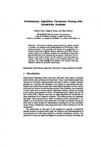
the blind algorithm to each instance and allow them to run for 2,000 secs. The proposed algorithms solve each instance 10 times for each value of (1 − 𝛼). Table 3 shows the results obtained by the local-search-based matheuristic methods for instances A, B, and C for four different values of (1 − 𝛼). As expected, the blind algorithm consistently obtains GAP values much higher than the other three methods. Further, local-search-based algorithms are able to find the optimal solution for the majority of the instances. While the average GAP for the blind algorithm is 1.65%, the average GAP for the SD, ND, and TS methods is 0.33%, 0.36%, and 0.15%, respectively. As expected, the best average value is obtained by the TS algorithm while difference between SD and ND algorithms is negligible. Regarding the time needed by the algorithms to converge, the blind algorithm
is the one that takes longer (770 secs). As mentioned before, the ND algorithm is, in average, the fastest one with 299 seconds, while the SD algorithm almost doubles this time with 547 seconds, in average. TS algorithm takes 371 seconds, in average, before convergence. Figures 4(a), 5(a), and 6(a) show the evolution of the GAP, as parameter (1 − 𝛼) increases. As we expected, the larger the value of (1 − 𝛼) is set to, the smaller the GAP. Also, it is clear that the blind algorithms obtain higher GAP values than the other three algorithms considered in this study. As we mentioned before, the blind algorithm works as our baseline algorithm. It is interesting to note that, for all algorithms, the worst performance is obtained for (1 − 𝛼) = 0.1. This is mainly because for this value not enough facilities are available and the algorithms open a set
Figure 5: Average results obtained by the local search algorithms for each value of (1 − 𝛼) for 𝑂𝑅𝐿𝑖𝑏 B instances.
1,000
6
800
4 Time (sec)
GAP value (%)
5
3
600
400
2 1
200 0
0
0.1
Blind SD
0.2
0.3
0.4 (1 − )
0.5
0.6
0.7
0.8
ND TS
(a) Evolution of the GAP for 𝑂𝑅𝐿𝑖𝑏 C instances
0
0.1
Blind SD
0.2
0.3
0.4 (1 − )
0.5
0.6
0.7
0.8
ND TS
(b) Evolution of the time for 𝑂𝑅𝐿𝑖𝑏 C instances
Figure 6: Average results obtained by the local search algorithms for each value of (1 − 𝛼) for 𝑂𝑅𝐿𝑖𝑏 C instances.
of facilities randomly so the problem has a feasible solution. However, this repairing process is completely random and, thus, algorithms performance is impaired. Since the problems from the OR Library are only medium size instances, local-search-based matheuristics consistently find the optimal solution for almost all instances for (1 − 𝛼) = {0.3, 0.5, 0.7}. In fact, even the blind algorithm finds solutions that are very close to the optimal ones when (1 − 𝛼) = 0.7.
Figures 4(b), 5(b), and 6(b) show the time needed by our algorithms to find its best solution, as parameter (1 − 𝛼) increases. Unlike we expected, the time needed to find the best solution does not increase as the parameter (1 − 𝛼) gets larger. In fact, both algorithms, SD and blind, converge faster when (1 − 𝛼 = 0.7), the larger value we tried in our experiments. This can be explained because of the problems features. We note that optimal solutions for all the
13
35
35
30
30
25
25 GAP value (%)
GAP value (%)
Complexity
20 15
20 15
10
10
5
5
0
0
0.1
Blind SD
0.2
0.3
0.4 (1 − )
0.5
0.6
0.7
0.8
ND TS
(a) Evolution of the GAP for DS1𝑈 instances
0
0
0.1
Blind SD
0.2
0.3
0.4 (1 − )
0.5
0.6
0.7
0.8
ND TS
(b) Evolution of the GAP for DS1𝐶 instances
Figure 7: Average GAP values obtained by the local search algorithms for each value of (1 − 𝛼) for DS1 instances.
problems in the benchmark of the OR Library need not too many warehouses to be open. Thus, when a large portion of the potential warehouses are available (as for the (1 − 𝛼) = 0.7 case) the algorithm is likely to find such optimal solutions in early iterations. In fact, for the vast majority of the experiments, optimal solution is found within the first 2 to 3 iterations. We now move on the DS1𝑈 and the DS1𝐶 benchmarks. As we noted before, these sets of instances are much larger and harder to solve than the problems in the OR Library we discussed above. Further, as the optimal solutions of these instances do not require too many warehouses to be open, the repairing procedure applied to the OR Library instances for (1 − 𝛼) = 0.1 does not have a great impact on the results. Thus, local-search-based matheuristics outperform the results obtained by the blind algorithm for all values of parameter 𝛼. Figures 7(a) and 7(b) show the GAP values obtained by the all four algorithms for instances DS1𝑈 and DS1𝐶, respectively. Just as in the OR Library instances, as the parameter (1−𝛼) gets larger, the GAP approximates to 0 for the all three localsearch-based matheuristic proposed in this paper. While for the DS1𝑈 instances both the TS and the ND algorithms reach GAP values very close to 0 for (1 − 𝛼) = 0.5 and (1 − 𝛼) = 0.7, for the DS1𝐶 instances the best value obtained by the TS and the ND algorithms is 0.71 and 0.61, respectively, for (1 − 𝛼) = 0.7. Notably, the ND algorithm performs slightly better than the TS for the DS1𝐶 instance when (1 − 𝛼) = 0.5, obtaining a best average value of 0.66 against the 1.42 obtained by the TS algorithm. In spite of that, we can note that the differences between the GAP obtained by both the ND and the TS algorithms when using (1 − 𝛼) = 0.5 and (1−𝛼) = 0.7 are negligible, just as in the OR Library instances.
Figures 8(a) and 8(b) shows the time needed by the all four algorithms to find their best solution for instances DS1𝑈 and DS1𝐶, respectively. As expected, as the parameter (1 − 𝛼) gets larger, longer times are needed by the algorithms to converge. This is important as one would like to use a value for (1−𝛼) such that minimum GAP values are reached within few minutes. Results in Figures 7 and 8 show, clearly, that there is a compromise between the quality of the solution found by the algorithms and the time they need to do so. Further, we know that this compromise can be managed by adjusting the value of parameter (1−𝛼). For the case of instances DS1𝑈 and DS1𝐶, such a value should be between 0.4 and 0.6. Moreover, for the case of the instances of the OR Library, parameter (1 − 𝛼) should be set around 0.3. It is interesting to note that while the size of instances DS1𝑈 and DS1𝐶 is equivalent, instances of the OR Library are much smaller. We can also note that instances that include clusters tend to take longer to converge. This is especially true as parameter (1 − 𝛼) gets larger. Further, for these instances, as the parameter (1 − 𝛼) gets larger, less iterations are performed by algorithms although each of these iterations takes much longer. As mentioned before, these should be taken into account when using population-based algorithms within the framework presented in this study as such kind of heuristic algorithms needs to perform several iterations before to converge to good quality solutions.
4. Conclusions and Future Work In this paper we show the impact of parameter tuning on a local-search-based matheuristic framework for solving
Complexity 2,000
2,000
1,800
1,800
1,600
1,600 Time (sec)
Time (sec)
14
1,400 1,200
1,400 1,200
1,000
1,000
800
800 0
0.1
Blind SD
0.2
0.3
0.4 (1 − )
0.5
0.6
0.7
0.8
ND TS
(a) Evolution of the time for DS1𝑈 instances
0
0.1
0.2
0.3
Blind SD
0.4 (1 − )
0.5
0.6
0.7
0.8
ND TS
(b) Evolution of the time for DS1𝐶 instances
Figure 8: Average times needed by the local search algorithms for each value of (1 − 𝛼) for DS1 instances.
mixed integer (non)linear programming problems. In particular, matheuristics that combine local search methods and a MIP solver are tested. In this study, we focus on the size of the subproblem generated by the local search method that is passed on to the MIP solver. As expected, the size of the subproblems that are solved in turn by the matheuristic method has a big impact on the behaviour of the matheuristic and, consequently, on its obtained results: as the size of the subproblem increases (i.e., more integer/binary decision variables are considered) the results obtained by the MIP solver are closer to the optimal solution. The time required by the algorithms tested in this paper to find its best solution also increases as the subproblem gets larger. Further, as the subproblem gets larger, fewer iterations can be performed within the allowed time. This is important as other heuristics such as evolutionary algorithms and swarm intelligence, where many iterations are needed before converging to a good quality solution, might be not able to deal with large subproblems. We also note that the improvement in the GAP values after certain value of parameter (1 − 𝛼) is negligible and that this value depends to some extent on the size of the problem: for medium size instances such as the ones in the OR Library, parameter (1 − 𝛼) should be set to a value around 0.3 while for larger instances (DS1𝑈 and DS1𝐶) it should be set to a value between 0.4 and 0.6. The specific values will depend on both the accuracy level requested by users and the time available to perform the algorithm. Therefore, the challenge when designing matheuristic frameworks as the one presented in this paper is to find a value for parameter (1 − 𝛼) that allows the heuristic algorithm to perform as many iterations as needed and that provides a good compromise between solution quality and run times. Although the values provided here are only valid for the
problem and the algorithms considered in this paper, we think that the obtained results can be used as a guide by other researchers using similar frameworks and/or dealing with similar problems. As a future work, strategies such as evolutionary algorithms and swarm intelligence will be tested within the matheuristic framework considering the results obtained in this study. We expect that intelligent methods such as the ones named before greatly improve the results obtained by the local search methods considered in this study. Moreover, the matheuristic framework used in this paper might also be applied to other MILP and MINLP problems such as, for instance, the beam angle optimisation problem in radiation therapy for cancer treatment.
Conflicts of Interest The authors declare that there are no conflicts of interest regarding the publication of this paper.
Acknowledgments Guillermo Cabrera-Guerrero wishes to acknowledge Ingenier´ıa 2030, DI 039.416/2017 and CONICYT/FONDECYT/ INICIACION/11170456 projects for partially supporting this research.
References [1] F. Neri and C. Cotta, “Memetic algorithms and memetic computing optimization: a literature review,” Swarm and Evolutionary Computation, vol. 2, pp. 1–14, 2012.
Complexity [2] Y.-s. Ong, M. H. Lim, and X. Chen, “Memetic Computation—Past, Present & Future,” IEEE Computational Intelligence Magazine, vol. 5, no. 2, pp. 24–31, 2010. [3] X. Chen, Y.-S. Ong, M.-H. Lim, and K. C. Tan, “A multifacet survey on memetic computation,” IEEE Transactions on Evolutionary Computation, vol. 15, no. 5, pp. 591–607, 2011. [4] V. Maniezzo, T. St¨utzle, and S. Voß, Eds., Matheuristics Hybridizing Metaheuristics and Mathematical Programming, vol. 10 of Annals of Information Systems, Springer, 2010. [5] G. Guillermo Cabrera, E. Cabrera, R. Soto, L. J. M. Rubio, B. Crawford, and F. Paredes, “A hybrid approach using an artificial bee algorithm with mixed integer programming applied to a large-scale capacitated facility location problem,” Mathematical Problems in Engineering, vol. 2012, Article ID 954249, 14 pages, 2012. [6] M. Caserta and S. Voß, “A math-heuristic Dantzig-Wolfe algorithm for capacitated lot sizing,” Annals of Mathematics and Artificial Intelligence, vol. 69, no. 2, pp. 207–224, 2013. [7] L. C. Coelho, J.-F. Cordeau, and G. Laporte, “Heuristics for dynamic and stochastic inventory-routing,” Computers & Operations Research, vol. A, no. 0, pp. 55–67, 2014. [8] C. Lagos, F. Paredes, S. Niklander, and E. Cabrera, “Solving a distribution network design problem by combining ant colony systems and lagrangian relaxation,” Studies in Informatics and Control, vol. 24, no. 3, pp. 251–260, 2015. [9] B. Raa, W. Dullaert, and E.-H. Aghezzaf, “A matheuristic for aggregate production-distribution planning with mould sharing,” International Journal of Production Economics, vol. 145, no. 1, pp. 29–37, 2013. [10] H. Allaoua, S. Borne, L. L´etocart, and R. Wolfler Calvo, “A matheuristic approach for solving a home health care problem,” Electronic Notes in Discrete Mathematics, vol. 41, pp. 471–478, 2013. [11] G. Cabrera-Guerrero, M. Ehrgott, A. J. Mason, and A. Raith, “A matheuristic approach to solve the multiobjective beam angle optimization problem in intensity-modulated radiation therapy,” International Transactions in Operational Research, 2016. [12] Y. Li, D. Yao, J. Zheng, and J. Yao, “A modified genetic algorithm for the beam angle optimization problem in intensitymodulated radiotherapy planning,” in Artificial Evolution, E.G. Talbi, P. Liardet, P. Collet, E. Lutton, and M. Schoenauer, Eds., vol. 3871 of Lecture Notes in Computer Science, pp. 97–106, Springer, Berlin, Germany, 2006. [13] Y. Li, D. Yao, W. Chen, J. Zheng, and J. Yao, “Ant colony system for the beam angle optimization problem in radiotherapy planning: a preliminary study,” in Proceedings of the 2005 IEEE Congress on Evolutionary Computation, volume 2, pp. 1532– 1538, IEEE, Edinburgh, Scotland, UK, September 2005. [14] S. Hanafi, J. Lazi´c, N. Mladenovi´c, C. Wilbaut, and I. Cr´evits, “New hybrid matheuristics for solving the multidimensional knapsack problem,” Lecture Notes in Computer Science (including subseries Lecture Notes in Artificial Intelligence and Lecture Notes in Bioinformatics): Preface, vol. 6373, pp. 118–132, 2010. [15] E.-G. Talbi, “Combining metaheuristics with mathematical programming, constraint programming and machine learning,” 4OR, vol. 11, no. 2, pp. 101–150, 2013. [16] C. Archetti and M. G. Speranza, “A survey on matheuristics for routing problems,” EURO J. in Computer Optimization, vol. 2, no. 4, pp. 223–246, 2014. [17] M. A. Boschetti, V. Maniezzo, M. Roffilli, and A. Boluf´e R¨ohler, “Matheuristics: Optimization, simulation and control,” Lecture
15
[18]
[19]
[20]
[21] [22] [23]
[24]
[25]
[26]
[27]
[28] [29]
[30]
Notes in Computer Science (including subseries Lecture Notes in Artificial Intelligence and Lecture Notes in Bioinformatics): Preface, vol. 5818, pp. 171–177, 2009. C.-H. Chen and C.-J. Ting, “Combining lagrangian heuristic and ant colony system to solve the single source capacitated facility location problem,” Transportation Research Part E: Logistics and Transportation Review, vol. 44, no. 6, pp. 1099– 1122, 2008. Y. Li, J. Yao, and D. Yao, “Automatic beam angle selection in IMRT planning using genetic algorithm,” Physics in Medicine and Biology, vol. 49, no. 10, pp. 1915–1932, 2004. Y. Li, D. Yao, J. Yao, and W. Chen, “A particle swarm optimization algorithm for beam angle selection in intensity-modulated radiotherapy planning,” Physics in Medicine and Biology, vol. 50, no. 15, pp. 3491–3514, 2005. F. Glover and M. Laguna, Tabu Search, Kluwer Academic Publishers, Norwell, MA, USA, 1997. M. Pirlot, “General local search methods,” European Journal of Operational Research, vol. 92, no. 3, pp. 493–511, 1996. C. Lagos, G. Guerrero, E. Cabrera et al., “A Matheuristic Approach Combining Local Search and Mathematical Programming,” Scientific Programming, vol. 2016, Article ID 1506084, 2016. V. Vails, M. A. Perez, and M. S. Quintanilla, “A tabu search approach to machine scheduling,” European Journal of Operational Research, vol. 106, no. 2-3, pp. 277–300, 1998. S. Hanafi and A. Freville, “An efficient tabu search approach for the 0-1 multidimensional knapsack problem,” European Journal of Operational Research, vol. 106, no. 2-3, pp. 659–675, 1998. J. Brand˜ao and A. Mercer, “A tabu search algorithm for the multi-trip vehicle routing and scheduling problem,” European Journal of Operational Research, vol. 100, no. 1, pp. 180–191, 1997. K. S. Al-Sultan and M. A. Al-Fawzan, “A tabu search approach to the uncapacitated facility location problem,” Annals of Operations Research, vol. 86, pp. 91–103, 1999. P. B. Mirchandani and R. L. Francis, Eds., Discrete Location Theory, Wiley-Interscience, New York, NY, USA, 1990. J. E. Beasley, “OR-Library: distributing test problems by electronic mail,” Journal of the Operational Research Society, vol. 41, no. 11, pp. 1069–1072, 1990. J. G. Villegas, F. Palacios, and A. . Medaglia, “Solution methods for the bi-objective (cost-coverage) unconstrained facility location problem with an illustrative example,” Annals of Operations Research, vol. 147, pp. 109–141, 2006.
Advances in
Operations Research Hindawi Publishing Corporation http://www.hindawi.com