www.nature.com/scientificreports
OPEN
received: 17 April 2015 accepted: 24 August 2015 Published: 23 September 2015
Parameterization of clearsky surface irradiance and its implications for estimation of aerosol direct radiative effect and aerosol optical depth Xiangao Xia Aerosols impact clear-sky surface irradiance (E g ↓ ) through the effects of scattering and absorption. Linear or nonlinear relationships between aerosol optical depth (τa) and E g ↓ have been established to describe the aerosol direct radiative effect on E g ↓ (ADRE). However, considerable uncertainties remain associated with ADRE due to the incorrect estimation of Eg0↓ (τa in the absence of aerosols). Based on data from the Aerosol Robotic Network, the effects of τa, water vapor content (w) and the cosine of the solar zenith angle (μ) on E g ↓ are thoroughly considered, leading to an effective parameterization of E g ↓ as a nonlinear function of these three quantities. The parameterization is proven able to estimate Eg0↓ with a mean bias error of 0.32 W m−2, which is one order of magnitude smaller than that derived using earlier linear or nonlinear functions. Applications of this new parameterization to estimate τa from E g ↓ , or vice versa, show that the root-mean-square errors were 0.08 and 10.0 Wm−2, respectively. Therefore, this study establishes a straightforward method to derive E g ↓ from τa or estimate τa from E g ↓ measurements if water vapor measurements are available.
Surface irradiance, the downwelling solar radiation from the Sun and sky that reaches the surface (E g ↓), is the ultimate energy source for the Earth’s climate system and life on the planet. A large number of diverse surface processes are governed by the amount of E g ↓; for example, evaporation, snow/glacier melt and plant photosynthesis. Therefore, E g ↓ plays an important role in studies of hydrological and carbon cycling1–3. Aerosols scatter and absorb solar radiation and thereby modulate the amount of clear-sky E g ↓ (E g ↓ hereafter). We define the aerosol direct radiative effect on E g ↓ (ADRE) as the attenuation of clear-sky E g ↓ due to aerosol scattering and absorption, i.e., the difference between E g ↓ and E g0↓ (E g ↓ in the absence of aerosols). ADRE is widely reported in the literature, based on a combination of measurements of E g ↓ and aerosol optical depth (τa)4–7. E g0↓ cannot be obtained straightforwardly from observations since the atmosphere almost has aerosols present. One of the difficulties relating to the derivation of ADRE stems from the need to accurately estimate E g0↓7,8. Radiative transfer model or single-layer clear-sky solar radiation model can be used to calculate E g0↓9–12 and thereby ADRE is obtained, however, this method is sensitive to the calibration uncertainties of pyranometer (independent of model calculation) and dependent on model assumptions about the atmospheric parameters13. E g0↓ can be estimated from observations, this method avoids dependence on a model, furthermore, ADRE estimation should not be very sensitive to the calibration errors since E g0↓ is derived from observations13. A linear relationship of E g ↓ to τa has been popularly assumed and E g0↓ is then derived by linear regression LAGEO, Institute of Atmospheric Physics, Chinese Academy of Sciences, Beijing, China. Correspondence and requests for materials should be addressed to X.X. (email:
[email protected]) Scientific Reports | 5:14376 | DOI: 10.1038/srep14376
1
www.nature.com/scientificreports/ 600
θs = 59.2 w = 0.6(cm) w = 2.7(cm)
(a)
550
θs = 74.5
(b)
−2
Eg↓ (W m )
500
450
400
Eg↓
E0
350
550.9 550.9 546.6 549.7 435.4
510.0 509.9 502.0 505.7 508.6
300
0
0
g↓
0.2
0.4
AERONET Y=A×exp(B×XC) Y=A+B×X Y=A×exp(B×X) Y=A*exp(B×X)+C 0.6 τa550nm
0.8
1
1.2
Eg↓
E0
260.3 260.3 252.5 255.7 259.0
237.5 237.5 226.8 231.1 236.7
g↓
0.2
0.4
AERONET Y=A×exp(B×XC) Y=A+B×X Y=A×exp(B×X) Y=A*exp(B×X)+C 0.6 τa550nm
0.8
1
1.2
Figure 1. Scatter-plot of aerosol optical depth (τa) and surface irradiance (E g ↓ ) for a solar zenith angle of (a) 59.2° and (b) 74.5°, and water vapor of 0.6 cm (red) and 2.7 cm (blue). These x-marks represent the Aerosol Robotic Network model calculation of surface irradiance in the absence of aerosols (Eg0↓). The values given in the first line represent the mean Eg0↓ by the Aerosol Robotic Network model calculation, and the following values are Eg0↓ derived on the basis of Eqs (1)–(4). The figure was produced using MATLAB.
analysis of E g ↓ and τa4,5,13. Some studies suggested that an exponential decay of E g ↓ with an increase in τa would be expected according to Beer–Lambert Law, which is especially true for cases with τa values larger than 0.57,8,13. However, contrary to expectation, a better estimation of E g0↓ was derived from the linear regression than using the exponential relationship. This was thought to be because the systematic underestimation of E g0↓ by the linear regression was compensated by the positive correlation between τa and water vapor content (w)8. In this study, we show that these previous methods produce a systematic bias in the derivation of E g0↓ and thereby result in an overestimation of ADRE. A new parameterization of E g ↓ is developed based on global Aerosol Robotic Network (AERONET) data, in which the relationships of E g ↓ to the cosine of the solar zenith angle (μ), τa and w have been established by using a combination of nonlinear equations. The results show that the mean bias error (MBE) of the estimations of E g0↓ decreases from 4–7 W m−2 to 0.32 W m−2. The same improvement in the estimation of ADRE would be expected when using the new method. Furthermore, one of the important advantages of this parameterization is that a straightforward method to derive τa from E g ↓, or vice versa, has been established. Specifically, we find it is possible to derive τa from E g ↓ with a root-mean-square error (RMSE) of 0.08, and vice versa with an RMSE of 10.0 W m−2.
Results
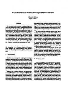
The solid dots in Fig. 1 represent the scatter between τa at 550 nm (τa hereafter) and E g ↓ at two narrow μ and w ranges. The analysis is firstly performed on data points with a very narrow range of μ (~0.2°) and w (10%w), to isolate the effect of τa on E g ↓. The mean E g0↓ amounts, using the AERONET calculation and fitting E g0↓ values using regression analysis on the basis of Eqs (1)–(4) in the Method section, are also presented. The performance of these equations is evaluated by the agreement in instantaneous E g0↓ between the AERONET calculations and the regression analysis results. We can see that the best performance is achieved using Eq. (4), the new parameterization proposed in this study, which produces a difference in E g0↓ between the mean AERONET calculation and the regression analysis result (∆E g0↓) of nearly zero. This nearly zero ∆E g0↓ is in fact always derived using Eq. (4) for the full μ and w ranges (not shown). In contrast, ∆E g0↓, when using Eqs (1), (2) and (3), varies from a few to tens of W m−2 in these two cases. The fact that Eq. (3) occasionally produces unrealistic results that indicate the poor performance of the nonlinear regression analysis8, we eliminate it hereafter. Poorer performance of Eqs (1) and (2) than Eq. (4) is further shown by the histogram of ∆E g0↓ for Eqs (1) and (2) given in Fig. 2. Both equations nearly always underestimate E g0↓. The mean bias error (MBE) and RMSE of E g0↓ estimations are 6.8 (2.6) W m−2 for Eq. (1) and 3.6 (1.9) W m−2 for Eq. (2). The fact that Eq. (1) produces a considerably poorer result than Eq. (2) clearly shows the superiority of using nonlinear regression to Scientific Reports | 5:14376 | DOI: 10.1038/srep14376
2
www.nature.com/scientificreports/ 600 (b) Eq. (2) MBE = 3.6 RMSE = 1.9
400
Occurrence Number
Occurrence Number
500
(a) Eq. (1) MBE = 6.8 RMSE = 2.6
300
200
100
0
−10
−5
0 0
−2 ∆Eg↓ (W m )
5
10
−10
−5
0
5
10
0
−2 ∆Eg↓ (W m )
Figure 2. Histogram of the difference in surface irradiance in the absence of aerosols between the Aerosol Robotic Network model calculations and regression results using Eqs (1) and (2) (∆Eg0↓ ). The given values are the mean bias and root-mean-square error of Eqs (1) and (2). The figure was produced using MATLAB.
extrapolate E g ↓ to zero τa rather than linear regression. This conclusion is also supported by the fact that smaller residuals of the regression analysis are derived from Eq. (2) than from Eq. (1). This is expected because attenuation of E g ↓ by aerosols shows nonlinear decay, as implied by Beer–Lambert Law. The difference between Eq. (2) and Eq. (4) is the introduction of a new parameter, C, into Eq. (4). The value of C is nearly always lower than 1.0 (the exact value of Eq. (3)), which is one of the most important reasons for the better performance of Eq. (4). Eq. (3) is somewhat similar to Beer–Lambert Law, which depicts the attenuation of solar direct radiation by aerosols; however, some part of the attenuation of solar direct radiation is backscattered to the surface, which is certain to enhance E g ↓. It is therefore expected that C should be lower than 1.0. In addition, the effect of aerosols on E g ↓ should not be independent from μ, since μ governs the transfer path of photons. This implies that C should vary with μ, which is reflected in the following analysis. Figure 3 presents the dependence of E g0↓ (A in Eq. (4)), on w and μ. Variation of E g0↓ is mainly governed by μ, which is somewhat modulated by w at the same value of μ. Therefore, parameter A for a given amount of w is firstly simulated using a power law function of μ (Eq. (5) in the Methods section). The first and most important reason for the selection of a power law function is because it models the simple physics of the situation with only two parameters14,15. Parameter a1 of Eq. (5) represents expected measurements of E g0↓ for a μ of 1. Parameter a2 governs the E g0↓ variation with μ. The second reason for selection of a power law function is that it provides a faithful approximation to the data. Since the dependence of E g0↓ on μ is depicted by parameters a1 and a2 of Eq. (5), the w effect on E g0↓ is further simulated through the parameterization of a1 and a2 as a function of w. Figure 4 shows the relationships of a1 and a2 to w. We can see that the effect of water vapor per one unit of w on E g0↓ decreases as w increases, which is expected since the relative increase in water vapor absorption gradually decreases as w increases16. These relationships are simulated using an exponential equation. The RMSEs of the regression analysis for a1 and a2 of Eq. (5) are 1.37 and 0.0004, respectively, indicating a faithful approximation. A parameterization of E g0↓ to μ and w can then be established through a combination of Eqs (5)–(7) that leads to Eq. (8). Therefore, it is straightforward to calculate E g0↓ from Eq. (8) if w is available, since μ can be calculated from location and time very accurately. Further analysis of parameters B and C of Eq. (4) shows that both parameters are moderately related to μ and w, which thereby leads to a parameterization of E g ↓ as a function of τa, μ and w. As shown in Fig. 5, parameters B and C are approximated well using Eqs (9) and (10). In terms of the variability of both parameters, 99.8% is explained by the regression analysis. Since the relationship between instantaneous E g ↓ to τa as well as w for a specified value of μ is established, therefore, a straightforward method is developed that can be used to derive E g ↓ if τa and w are available from another source, such as satellite Scientific Reports | 5:14376 | DOI: 10.1038/srep14376
3
www.nature.com/scientificreports/ 800
4 E0 = 1226.27µ1.13 (w=0.20) g↓ 0
700
1.18
Eg↓ = 1094.41µ
3.5
(w=4.02)
3
E0g↓ (W m−2)
600
2.5
500
2
400
1.5 300 1 200 0.5 100
0.2
0.3
0.4 µ
0.5
0.6
Figure 3. Scatter-plot of the cosine of the solar zenith angle (μ) and surface irradiance in the absence of aerosols (Eg0↓ ). The color bar represents the water vapor content (cm). The curve represents the regression result for a specified water vapor content of 0.20 cm (blue) and 4.02 (red). The figure was produced using MATLAB.
1.18
1240 (a)
(b) 1.175
1220
1.17 1200 1.165
1160
1.155
2
1.16 a
a1
1180
1.15
1140
1.145 1120 1.14 1100 a = 1350.28× exp(−0.148×w0.25) 1 RMSE = 1.37 1080 1 2 3 w (cm)
0.15
a = 1.05× exp(0.091×w 2 RMSE = 0.000426 4
1
2 w (cm)
)
1.135 3
4
1.13
Figure 4. Scatter-plot of water vapor content and parameters (a) a1 and (b) a2 ofEq. 5. The curve represents the regression result using Eqs (6) and (7). The figure was produced using MATLAB.
remote sensing. On the other hand, it can also be used to derive τa if E g ↓ and w are available from sources such as the Baseline Surface Radiation Network (BSRN). The proposed method is evaluated by using the 20% of validating data and BSRN data at Xianghe. Figure 6a shows the comparison of instantaneous AERONET E g0↓ values of validating data and calculations from Eq. (8) based on validating AERONET τa and w. The MBE is 0.33 W m−2, one order magnitude smaller than the results from Eq. (1) and (2), even though the latter is derived from the training data. Since E g0↓ is simulated well by Eq. (5), the ADRE derivation based on Eq. (5) should be very close to that derived from the AERONET model calculations. This expectation is supported by Fig. 6b, in which the AERONET ADREs are compared with estimations from Eq. (8). The MBE and RMSE values are − 0.32 and 2.52 W m−2, respectively. To test the effectiveness of the parameterization of E g ↓, the instantaneous AERONET τa and w values from the testing data points are substituted into Eqs (8)–(10) to estimate E g ↓ values that are then compared with the AERONET E g ↓ products. Similarly, τa values are estimated from AERONET E g ↓ and w Scientific Reports | 5:14376 | DOI: 10.1038/srep14376
4
MBE = 0.0005 −0.3
RMSE = 0.04
−0.4 −0.5 −0.6 −0.7 −0.8 −0.9
(a) −0.8
−0.6 −0.4 B of the Eq. (4)
−0.2
Parmaterization by using the Eq. (10)
Parmaterization by using the Eq. (9)
www.nature.com/scientificreports/ 1.05 1
MBE = 0.0000
60
RMSE = 0.03
50
0.95
40
0.9
30
0.85
20
0.8
10 (b)
0.75
0.8
0.9 C of Eq. (4)
1
Figure 5. Density plot of parameters (a) B and (b) C of Eq. 4 and their parameterization results using Eqs (9) and (10). The color scale represents the relative density of points, where orange to red colors (levels ~45‒60) indicate the highest number density. The mean bias error and root-mean-square error of the parameterization are also included. The figure was produced using MATLAB.
0
MBE = 0.32
ADRE from the paramertization
800
g↓
E0 using the Eq. (5)
700 RMSE = 2.52 600 500 400 300 200 100
(a) 200
400
AERONET
600 0 Eg↓
800 −2
(W m )
MBE = −0.32
60
RMSE = 2.52
50
−50
40 −100
30 20
−150
10 −200 −200
(b) −150
−100
−50
0 −2
AERONET ADRE (W m )
Figure 6. Density plot of AERONET (a) Eg0↓ and (b) ADRE and their parameterization results using Eqs (8). The color scale represents the relative density of points, where orange to red colors (levels ~ 45‒60) indicate the highest number density. The mean bias error and root-mean-square error of the parameterization are also included. The figure was produced using MATLAB.
values and compared with AERONET τa products. Figure 7a shows that E g ↓ can be estimated with an MBE and RMSE of 0.02 and 10.0 W m−2, respectively. This certainly relies on the fact that both τa and w are available. On the contrary, if w and E g ↓ are available and τa is not known, τa can be retrieved from E g ↓ and w using this parameterization. The MBE and RMSE values of τa retrievals are 0.0005 and 0.08, respectively (Fig. 7b). Measurements of E g ↓ and τa at Xianghe7, a BSRN and AERONET station in China are used to further evaluate the effectiveness of the parameterization of E g ↓. The results are shown in Fig. 8. The estimations of E g ↓ from AERONET τa and w products using the proposed parameterization method agree with the BSRN measurements very well, with an MBE and RMSE of − 3.9 and 12.5 W m−2, respectively. On the other hand, the retrievals of τa from the measurements of E g ↓ and w are compared with AERONET τa products and the MBE and RMSE values are − 0.03 and 0.08, respectively. These results once again proved the reliability of the proposed parameterization method.
Uncertainty analysis. In the parameterization of E g0↓ (Eq. 8 of the Method section), surface albedo effect was excluded that likely produced bias in the estimation of E g0↓. Figure 9 shows the scatter-plot of Scientific Reports | 5:14376 | DOI: 10.1038/srep14376
5
www.nature.com/scientificreports/ 2
700
MBE = 0.0005
RMSE = 10.01
60
RMSE = 0.08
50
1.5
600 Estimated τa
Estimated Eg↓ (W m−2)
MBE = 0.02
500 400 300
40 1
30 20
0.5
200 100
10
(a) 200
400
0
600
AERONET E
g↓
(b) 0
−2
(W m )
0.5 1 1.5 AERONET τ
2
a
Figure 7. Density plot of AERONET (a) E g ↓ and (b) τa and their parameterization results using Eqs (8‒10). The color scale represents the relative density of points, where orange to red colors (levels ~ 45‒60) indicate the highest number density. The mean bias error and root-mean-square error of the parameterization are also included. The figure was produced using MATLAB.
2
700
MBE = −0.0310
RMSE = 12.54
60
RMSE = 0.08
50
1.5 a
600 Estimated τ
Estimated E
g↓
(W m−2)
MBE = −3.94
500 400 300
40 1
30 20
0.5
200 100
(a) 200
400
600 −2
AERONET Eg↓ (W m )
10 0
(b) 0
0.5 1 1.5 AERONET τ
2
a
Figure 8. Similar as Fig. 7 but for the results from AERONET and BSRN data at Xianghe. The figure was produced using MATLAB.
surface albedo and ∆E g0↓, from which we can see a significant negative correlation between both quantities. Uncertainty of 0.1 in surface albedo may produce 1–3 W m−2 bias in E g0↓. τa is the dominant aerosol optical property driving the variation of E g ↓ and therefore ADRE. However, aerosol absorption also plays an important role in ADRE17, which shows a wide range of variations and thereby may lead to uncertainties in the parameterization of E g ↓, since it was not accounted for. Remarkable impact of aerosol single scattering albedo at 550 nm (ω550nm) on the estimation of E g ↓ is presented in Fig. 10. E g ↓ changes as a result of uncertainty of ω550nm (0.03) was estimated to be a few Wm−2 that depends on optical path and τa. Significant impacts of ω550nm on estimation of E g ↓ from τa are further evidenced in Fig. 11 in which ∆E g0↓ shows a significant correlation to ω550nm. The best estimation is achieved for ω550nm of ~0.90 that is close to the median value of ω550nm of AERONET data points. In the above error analysis of E g0↓, water vapor is assumed to be known without any uncertainty. This is, of course, not realistic, since water vapor products from AERONET, satellite measurements are not free of uncertainty. By differentiating Eq. (8) with respect to w, the uncertainty of E g0↓ is estimated to be