A regional-scale land surface parameterization

Hydrological Sciences—Journal—des Sciences Hydrologiques, 43(4) August 1998 Special issue: Monitoring and Modelling of Soil Moisture: Integration over Time and Space

611

A regional-scale land surface parameterization based on areally-averaged hydrological conservation equations M. L. KAWAS, Z.-Q. CHEN & L. TAN Department of Civil & Environmental Engineering, University of California, Davis, California 95616, USA e-mail: [email protected]

S.-T. SOONG Atmospheric Science Program, LAWR, University of California, Davis, California 95616, USA

A. TERAKAWA, J. YOSHITANI & K. FUKAMI Public Works Research Institute, Ministry of Construction, 1 Asahi, Tsukuba, Ibaraki, 305 Japan Abstract In order to account for subgrid-scale spatial variability (heterogeneity) of land surface characteristics in regional-scale hydrological-atmospheric models, a land surface parameterization of areally-averaged sensible heat and évapotranspiration fluxes which is based upon areally-averaged hydrological soil water flow and soil heat flow equations, was developed. This land surface parameterization is fully coupled in a two-way interaction with the atmospheric boundary layer and the regional atmospheric model's first layer. The Monin-Obukhov similarity theory which is utilized in modelling the atmospheric boundary layer, and the areallyaveraged hydrological conservation equations are strictly valid only over stationaryheterogeneous areas where the fluctuations of the hydrological and boundary layer state variable values, parameter values, and of boundary conditions have spatially invariant means, spatially invariant higher moments and spatially invariant probability distributions. Therefore, the coupled two-way interactive model was run first for the computation of land surface fluxes over stationary-heterogeneous land patches, each corresponding to a single soil texture-vegetation class. Then, utilizing a mosaic scheme, the land surface fluxes over a regional model grid cell were obtained by numerical probabilistic averaging. The application of the regional model with this land surface parameterization to California during April 1989 has produced promising results.

Paramétrisation du territoire à l'échelle régionale basée sur les équations de conservation hydrologique Résumé Pour tenir compte de la variabilité des caractéristiques de surface d'un territoire à une échelle inférieure à celle du maillage du modèle régional couplant phénomènes hydrologiques et atmosphériques, nous avons développé une paramétrisation des moyennes surfaciques des flux de chaleur sensible et d'évapotranspiration basée sur les équations des flux d'eau et de chaleur dans le sol. Cette paramétrisation de la surface du sol repose sur l'interaction avec la couche limite atmosphérique et la première couche du modèle atmosphérique régional. La théorie de Monin-Obukhov qui a été utilisée pour modéliser la couche limite atmosphérique et les équations de conservation hydrologiques moyennées spatialement ne sont strictement applicables que sur des aires hétérogènes stationnaires où les fluctuations des variables d'état hydrologiques et de celles de la couche limite, les paramètres et les conditions aux limites possèdent des moyennes, des moments et des distributions de probabilité spatialement invariants. Par conséquent, le modèle couplé a d'abord

Open for discussion until 1 February 1999

612

M. L, Kavvas et al.

été utilisé pour le calcul des flux sur des parcelles de terrain hétérogènes mais stationnaires correspondant à différentes classes de texture de la végétation. Les flux selon le maillage du modèle régional ont été obtenus en effectuant numériquement une moyenne probabiliste à partir de la mosaïque des classes élémentaires de végétation. L'application du modèle régional utilisant cette paramétrisation des états de surface en Californie pour le mois d'avril 1989 a fourni des résultats satisfaisants,

INTRODUCTION The component of the earth-atmosphere system that is of great concern to human welfare is the interface between the atmosphere and the land surfaces. The heat and moisture exchanges between the earth surface and atmosphere are not only crucial for the atmospheric dynamics but they also determine the earth surface conditions, such as temperature, relative humidity and land surface wetness which are of utmost importance to the biosphere. The processes which take place at the interface between the earth surface and atmosphere such as infiltration, évapotranspiration and sensible heat exchange, are "land surface processes". Shukla & Mintz (1982), among others, have shown that the land surface fluxes to the atmosphere have profound influence on simulation results of climate models. Hence, it was recognized that it is important to parameterize the subgrid-scale land surface processes within climate models in a realistic fashion in order to improve their climate simulation results. Here, we define "scale" as the grid size of numerical computations and observations for hydrological-atmospheric processes. In the case of bare soil surfaces the latent heat and sensible heat flux parameterizations in General Circulation Models (GCMs) were achieved by following the Deardorff (1972) scheme where soil is represented in two layers, the top layer being a thin layer while the bottom layer acts as the heat or water storage. In the more general case of vegetated soil surfaces Dickinson et al. (1986), Sellers et al. (1986, 1997), and Noilhan & Planton (1989) have developed land surface parameterizations based on the big leaf scheme of Deardorff (1978). However, all of the above land surface parameterization schemes assume areal (horizontal) homogeneity of soils and vegetation within the grid area of the atmospheric model where they are calculating the sensible and latent heat fluxes. "Heterogeneity" may be defined as the fluctuations in the values of hydrological-atmospheric state variables (such as infiltration rate, évapotranspiration rate, relative humidity, potential temperature, etc.), hydrological-atmospheric parameters (such as hydraulic conductivity, porosity, albedo, surface roughness height, etc.) and in the boundary conditions/forcing functions (such as rainfall etc.) at a range of space and time scales. Heterogeneity may be classified into two major categories of stationary heterogeneity, and nonstationary heterogeneity. Stationary heterogeneity of a hydrological-atmospheric attribute occurs when the mean, the higher order statistical moments and the probability distribution functions for the attribute's fluctuations in time/space are invariant with respect to all time/space origin locations. A hydrological-atmospheric attribute is second order stationary-heterogeneous if its mean and variance/covariance do not vary with time/space origins, are finite, and the covariance is only a function of the time/space lag (or vectorial displacement in the case of multiple dimensions). A hydrological-atmospheric attribute is nonstationary-

A regional-scale land surface parameterization

613

heterogeneous if the mean, the higher order statistical moments and the probability distributions of this attribute's fluctuations vary with time/space origin locations. Since a typical grid area of a mesoscale atmospheric model (MAM) is of the order of 100 km2 and a typical grid area of a GCM is of the order of 100 000 km2, the heterogeneity in soil texture, vegetation cover and land topography is very pronounced over a typical grid area of a MAM or a GCM. Wetzel & Chang (1988) found that for numerical weather prediction models with a grid spacing of 100 km or greater, the expected subgrid-scale variability of soil moisture may be as large as the total amount of potentially available water in the soil. Also, the above mentioned soil-vegetation models consider homogeneous canopy characteristics (in terms of a single stoma) over each computational grid, thereby neglecting subgrid-scale areal variation in the vegetated portion of a computational grid of a MAM or a GCM. Recognizing these difficulties with the aforementioned schemes, several researchers attempted to develop land surface parameterization schemes which can account for the influence of subgrid-scale areal heterogeneity in soils and vegetation on the computation of land surface fluxes over a grid area of a MAM or a GCM. Avissar & Pielke (1989) divided each grid cell of a numerical model into homogeneous land patches, the so-called "mosaic pattern". Each homogeneous land patch was interpreted to represent one soil-vegetation class, and did not account for the heterogeneity within the particular patch. Patches of the same class, located at different places within the grid area, were regrouped into one subgrid soil-vegetation class. Avissar & Pielke (1989) then found the probability of occurrence of each soil-vegetation class for that grid by dividing the area which is occupied by the particular soil-vegetation class in that grid, by the grid area. They then obtained the average flux from a grid cell by multiplying the vertical flux from each particular soil-vegetation class by the probability of occurrence of that class within the grid and summing the products over all the soil-vegetation classes which are present within that grid. Later, Avissar (1991) accounted for the intra-patch heterogeneity within a soil-vegetation class by assuming probability density functions (pdfs) for the spatial variability of each of the parameters for that particular class. He numerically averaged the vertical fluxes, obtained by pointscale conservation equations, by means of the pdfs of soil-vegetation parameters in order to obtain the average vertical fluxes for that particular soil-vegetation class. He then followed the approach of Avissar & Pielke (1989) in order to obtain the average fluxes over the area of a grid cell. This approach is scientifically sound since it does average (numerically) the point-scale conservation equations by accounting for the spatial heterogeneity in the soil-vegetation parameters. Point-scale conservation equations are those which are based on mass/momentum/energy conservations at the scale of a differential control volume. Hence, they are at the scale of a spatial point location. Other approaches were developed by Entekhabi & Eagleson (1989), and Famiglietti & Wood (1991). Entekhabi & Eagleson (1989) assumed a probability density function for the spatial variability of soil water content in describing soil moisture flows within a GCM by means of point-scale hydrological conservation equations. Famiglietti & Wood (1991) considered a statistical distribution of a topography-soils index in order to account for the subgrid-scale variability in topography and soils within a GCM grid cell.

614

M. L. Kavvas et al.

Although, as mentioned above, there are already valuable studies on the modelling of subgrid-scale heterogeneity of land surface processes, a general theoretical framework on the modelling of these processes with heterogeneity at changing spatial scales is yet to be developed. However, such a theoretical framework is necessary to guide both the development of physically-based land surface process descriptions within mesoscale hydrological-atmospheric models and GCMs, and the observational activities on these processes (such as the GEWEX experiments). Toward development of such a theoretical framework, an approach which was taken by the authors, is the modelling of hydrological processes at changing spatial scales by means of the areally-averaged hydrological conservation equations at those scales, starting from the standard point-scale forms (at the scale of a spatial point location) of these equations (Kavvas & Govindaraju, 1992; Chen et al, 1993, 1994; Tayfur & Kavvas, 1994; Home & Kavvas, 1997). Areal averaging of a hydrological conservation equation is fundamentally equivalent to the areal integration of the equation and then the division of the resulting integral by the size of the area. Areally-averaged hydrological conservation equations, if they could be obtained in analytical forms at the grid scale of a mesoscale atmospheric model (MAM) or, ultimately, at the grid scale of a GCM, will have several significant advantages. First, such an areally-averaged conservation equation will contain information on the subgrid behaviour of the particular hydrological process over any grid area of a MAM (or GCM). Secondly, since they are in analytical forms (instead of the numerically-averaged values of the point-scale conservation equations, as in Avissar (1991)), they can be coupled directly with the MAM through the boundary layer. Such coupling can speed up the climate simulations of a coupled mesoscale hydrological-atmosphere model significantly. Thirdly, the analytical form of the areally-averaged conservation equation of a particular hydrological process shows clearly which state variable form (areal mean, areal variance, areal covariance, etc.) and which hydrological parameter form (e.g. areal mean and areal variance of hydraulic conductivity) need to be computed and estimated at the particular computational grid scale of a MAM (or GCM). Below, a land surface parameterization which is based upon areally-averaged hydrological conservation equations is presented.

DESCRIPTION OF THE LAND SURFACE PARAMETERIZATION In order to calculate the latent heat flux from land surfaces it is necessary to calculate évapotranspiration (ET). The total ET flux over an area which is made up of a homogeneous vegetation cover and a homogeneous soil, can be calculated as: ET = (\^veg)Eg+veg{Evd+Elr)

(1)

where veg denotes the fraction of the area which is vegetated, Eg is the bare-ground evaporation, Evd is the direct evaporation from vegetation leaves, and Etr is the vegetation transpiration over a homogeneous area. The bare-ground evaporation Eg can be estimated by the classical aerodynamic formula (Noilhan & Planton, 1989):

A regional-scale land surface

parameterization

615

Eg = PaCHVa(z)lhu(So)qSM(Ts) - qa(z)]

(2)

where pa is the air density; Va(z) and qa(z) are respectively the wind speed and specific humidity at height z, taken as the height of the first atmospheric layer of the atmospheric model; qSM (Ts) is the saturated specific humidity at the land surface temperature Ts; and hu(s0) is the relative humidity at ground surface which can be expressed as function of soil water saturation s0 at soil surface (Noilhan & Planton, 1989). The bulk transfer coefficient CH is dependent upon the surface boundary layer stability of the atmosphere and may be expressed by the Monin-Obukhov surface similarity theory (Stull, 1988) by:

""rfl(z)(e(z)-e.J

(3)

where u* and 9* are respectively the turbulence velocity scale and temperature scale, 0(z) is the potential temperature at the first atmospheric layer and 9S0 is the air potential temperature at the roughness height z0. The direct evaporation from vegetation leaves, Evd, can be calculated by: Evd = hvd(Wr)paCHVa(z)[q^Ts) - qa(z)]

(4)

where hvd (Wr) is the water availability for evaporation from the plant leaves which are covered by intercepted water. As such, it may be expressed as (Noilhan & Planton, 1989):

KAK) = WKmJm

(5)

in terms of the foliage water storage amount Wr and the canopy water holding capacity Wnmx. Adopting the Deardorff formulation (1978) for the interception storage equation, the time evolution of Wr may be expressed by: dWr - ^ = Pr- Ev + E„ - R„ with Wr < Wmax

(6)

where Pr is the precipitation rate, Ev is the evaporation from vegetation when positive and dew flux when negative, Elr is the transpiration rate and Ru is the throughfall rate from the interception storage which occurs when Wr > Wmi%. The canopy transpiration rate Etr may be computed again by an aerodynamic formula: E„ = hvtPaCHVa(z)ksÀTs) - qa(z)]

(7)

where the water availability parameter for transpiration, hvt, may be expressed as (Noilhan & Planton, 1989):

K, = (^~Kj)RJ(Ra + RJ for Ep > o

(8)

where Ep is the potential evaporation, expressed by the right-hand sides of equations (4) and (7) without the water availability parameters hvd or hvt; Ra is the aerodynamic resistance equal to l/paVa(z)CH; and Rs is the surface resistance which is expressed by Noilhan & Planton (1989) in terms of the mean water content of the soil column under consideration, and in terms of the effects of photosynthetically

616

M. L. Kavvas et al.

active radiation, the vapour pressure deficit of the atmosphere and air temperature. Hence, according to Noilhan & Planton (1989) hvl - hvt(u*, q*, s) where s is mean soil water saturation with respect to soil depth. However, if one desires to account explicitly for the effect of soil moisture dynamics on transpiration, one can also define the water availability parameter hvl in terms of the plant root water uptake (Feddes et al., 1976). By the root water uptake formulation, hvl can be expressed as:

hrl=ix(s0,Ep)

min(Z, , £ , )

f-*-

(9)

X

when the soil water flow continuity equation with root-water uptake as a sink term is integrated vertically under the Green-Ampt model formulation. In equation (9) u.(50, Ep) is the transpiration efficiency function which was defined rigorously by Feddes et al. (1976), Lr is the root depth, Lt is the soil water front depth, and s0 is soil surface water saturation. More detail on this result will be provided later. The sensible heat flux Hs from/onto land surfaces can be calculated again by the classical aerodynamic formula (e.g. Haltiner & Williams, 1980): Hx=cpPaCHVa(z)[dm-Qa(z)]

(10)

where cp is the specific heat of air at constant pressure, Qa(z) is the potential air temperature at the first atmospheric layer, and the potential air temperature Qso at the surface roughness height z0 is expressed as (Deardorff, 1974): T, Q*(u*z0YM Q = 1 + 0.0962— (11) s K } " 0.286P/1000 KV v ) where Ps and Ts are respectively the atmospheric pressure and temperature at the surface, K is the von Karman constant and v is kinematic viscosity. As seen from the formulations above for évapotranspiration and sensible heat flux, in order to be able to compute these fluxes from/onto land surfaces it is necessary to solve for the boundary layer dynamics in terms of its state variables u* and 0*. With Monin-Obukhov similarity theory u* and 0* can be calculated by (Haltiner & Williams, 1980): 0*

o(z) = e,„ + — lnf~-yh o

K

Z u* u{z) = — In— K z0

V

' "iî)_

Œ]

(12)

(13)

where the height z may be taken at the first layer of the atmospheric model, and the Monin-Obukhov similarity height L is a function of both u* and 9* (L = L(u*, 0*)). The correction terms \\ih and \\jm for the boundary layer, whose formulations are given by Lettau (1979), are again functions of u* and 9* through L. However, in order to solve these nonlinear equations for u* and 9*, it is still necessary to solve for the land surface temperature Ts. However, as shall be seen in the following, Ts is


parameterization

617

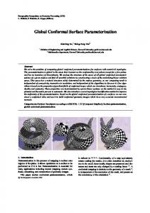
an outcome of the heat budget of the land surface which, in turn, varies with ET and sensible heat fluxes, as well as with the ground heat flux which itself is a function of the state of soil moisture. As such, the land/atmosphere system is a nonlinear system with very strong feedbacks between the land surface processes and atmospheric processes. These feedbacks are depicted in Fig. 1 which shows the dynamic coupling of the land surface processes with the atmospheric processes. In Fig. 1, in addition to the variables which were defined earlier, q(-) denotes specific humidity profile, P denotes precipitation, R„ denotes net radiation, ws denotes water content at the soil surface, G denotes ground heat flux, 9, and qx are the potential temperature and specific humidity at the first atmospheric layer, and F9ai and Fqai are respectively the vertical turbulence heat and moisture flux divergences at the first atmospheric layer which is taken at a = 0.995 atmospheric pressure in our model. Consequently, a realistic way for the prediction of the ET and sensible heat fluxes is to solve all the land/atmosphere system equations together in a completely coupled way. This is the approach taken in this study. Over a homogeneous area the ground surface temperature Ts can be calculated by means of the ground surface energy budget equation: dT

C ~L = S(l-a) dt

+ Fl-Fl-^LrET-Hs

+G

(14)

where, in addition to those variables which were defined earlier, C. is the heat

Feai(u.,e.,e,,e2)

Fv,i(u«,e.,qitq2)

First Atmospheric Layer (a = 0.995, z « 50m)

Constant flux Boundary Layer

Roughness height z„

Pure Diffusion Zone Soil surface z=0

T,(R„,E,HbG)

Soil Vadose Zone Soil water saturation G(T„ T»,,) profile Fig. 1 A schematic description of the two-way-interactive coupling of land surface hydrological processes with atmospheric processes.

618

M. L. Kavvas et al.

capacity of the soil, S is incoming solar radiation, a is surface albedo, F-l and F t are respectively the incoming and outgoing longwave radiation into/from the earth, and Lv is the latent heat of vaporization. It is important to note that this equation is applicable strictly to a horizontally homogeneous area. However, due to the spatial heterogeneity of soils, vegetation, topography and of atmospheric turbulence even over a land patch which represents one soil texture class and one vegetation class, the surface temperature, the radiation components, the turbulent heat fluxes and ground heat flux will all vary with point locations over this patch area. An individual model grid-cell area which is made up of a mosaic of these patches, will of course have more spatial variation of the above mentioned processes over such an area. Therefore, in order to have the scale of computed fluxes and of the hydrological processes to be consistent with the scale of a mesoscale atmospheric-hydrological model (MAM) grid-cell area it is necessary to areally average the surface energy budget equation together with all of its components first over each of the land patches (each representing one soil texture and one vegetation class) and then average the resulting mosaic pattern over the grid-cell area. The areal averaging of physical processes from point-scale toward the grid-scale of a MAM is fundamentally a two-stage process. The first stage in this integration process involves transforming the point-scale process conservation equations to their areally-averaged forms over stationary-heterogeneous regions which correspond to land patches of one soil-vegetation class. In the case of soil water flows a stationaryheterogeneous region is the one where the flow parameters, such as saturated hydraulic conductivity, and boundary conditions, such as precipitation, fluctuate in space around spatially-invariant means, and their fluctuations have spatially-invariant higher statistical moments (variance, covariance, skewness, etc.) over the region. The stationary-heterogeneity over a land patch is the same as the "intra-patch heterogeneity" of Avissar (1991). Avissar (1991) averaged the point-scale hydrological conservation equations numerically over each stationary-heterogeneous land patch. In contrast to this numerical averaging approach, here, we seek to obtain the analytical forms of the hydrological conservation equations when their point-scale forms are areally-averaged over stationary-heterogeneous land patches. It is also important to note here that the Monin-Obukhov similarity model of boundary layer dynamics is valid strictly for homogeneous turbulence. This means that it will be valid in modelling the momentum and potential temperature vertical profiles which are necessary for modelling the land surface fluxes (see equations (2), (3), (4), (7), (8), (9), (10), (11), (12) and (13)), only over stationary-heterogeneous regions. Therefore, the areally-averaged land surface fluxes and other hydrological state variables need to be computed in a two-way interactive, coupled manner with the atmospheric processes first over each stationary-heterogeneous land patch, corresponding to a single soil texture-vegetation class (as depicted in Fig. 1). In the second stage of averaging, it is assumed that horizontal fluxes among stationary-heterogeneous land patches are small as compared to the vertical fluxes within the large grid area of a MAM (-100 km2) (Avissar & Pielke (1989)).Then by following Avissar & Pielke's (1989) procedure, the stationary-heterogeneous regions belonging to the same class are grouped together within a MAM computational grid


619

cell. Then the average flux from the grid cell is calculated by multiplying the flux from each soil-vegetation class by the probability of occurrence of the particular class within the grid cell, and summing the products over all classes present in the particular grid cell. Within this framework the ground surface energy balance at the scale of a stationary-heterogeneous land patch, corresponding to a single soil-vegetation class, becomes an areally-averaged conservation equation expressed as: psi ff

\

Cg - ^ = (S(l - a)) + (FI -F t ) - Lv (ET) - (HS) + (G)

(15)

where ( ) denotes the areal averaging operator. As seen from equation (15), in order to compute the areal average soil surface temperature it is necessary to obtain the areallyaveraged values of the net shortwave radiation, the incoming and outgoing longwave radiation, the évapotranspiration, the sensible heat flux and the ground heat flux. The net shortwave radiation when expanded by Taylor series around areal average shortwave radiation (S) and areal average albedo (a), becomes to zeroth order: ( 5 ( l - a ) ) = (5)(l-)

(16)

In our model Stull's (1988) parameterization for shortwave radiation S = S* Tk sin \\i where S* is the solar irradiance, Tk is the net sky transmissivity and \\i is the local solar elevation angle, is being utilized. However, in order to develop an areal average shortwave radiation expression it is necessary to account for the spatial variation of incident solar radiation as function of aspect and slope, as was described by Obled & Harder (1978). This work shall be performed in the future, utilizing topographic data. Meanwhile, in the model described here, the areal average albedo is estimated from the land surface conditions. The net longwave radiation Fl - F t is computed in our model by the van Ulden & Holtslag (1985) formula: F I - F t = -87;4 (i - df ) + 407;3 (T; - r j

(17)

where J, is the temperature at the first atmospheric layer of the atmospheric model, 8 is the Stefan-Boltzman constant and C = 9.53 x 106 K2, an empirical constant. However, in order to arrive at an areally-averaged net longwave radiation it is necessary to account for the effect of topography, such as the shadowing effect (Marks, 1978). This work is expected to be performed in the future. The ground heat flux G is expressed by: (18) where X is the thermal conductivity of the soil in the z direction, s is the soil water

M. L. Kavvas et al.

620

saturation and T(z, t) is the soil temperature as function of depth and time. To zeroth order approximation the average heat flux can be expressed as:

-(x((s(Z,t))4d{T)

(G) =

(19)

dz

From equation (19) it is seen that in order to calculate the average heat flux (G), it is necessary to estimate the areal average thermal conductivity (X) as function of areal average soil water saturation \s(z, t)), and to calculate the areal average soil temperature gradient d(T)/dz . However, in order to calculate this gradient it is necessary to solve the areally-averaged form of the point-location-scale heat flow equation (Kirkham & Powers, 1984): ÔT

d

c

dT X(

)

(20)

" dt dz dz under the appropriate boundary conditions. In equation (20) Cg is the volumetric heat capacity of soil and other variables are as defined before. Utilizing the recent theory on the ensemble averaging of diffusion-type stochastic partial differential equations (Kavvas & Karakas, 1996), the exact second order ensemble average heat flow equation is expressed as:

'w

'

dt

a

8m {x(M,,)) s V1 /;

Cx dz d +

, IdT

dz i

'

t

C,X

dz

r r^COV

„, p,2

dz2

i ^

d(T)

(2D

dz

Therefore, in order to calculate the areally-averaged heat flux over a stationaryheterogeneous land patch, one first needs to solve equation (21) with the boundary conditions (T(z,t)) = (TX) for z = 0 , t > 0 and

(22) lim{j(z,0) = 0 f o r / > 0

However, as seen from equation (22) the solution of \T(z,t)) is dependent on the soil surface temperature \TX). Therefore, it is necessary to solve the soil heat flow equation simultaneously with the soil surface heat balance equation. Also, from equation (21) it can be seen that the areally-averaged thermal conductivity is a function of areally-averaged soil water saturation (s). McCumber & Pielke (1981) provide an expression which relates the thermal conductivity to the soil water saturation. From equation (21) it can also be seen that one needs to know the covariance of the soil thermal conductivity for the solution of equation (21). To the authors' knowledge, in the literature this covariance function has not been estimated yet from the field observations. If this covariance is not known, then the best one can


parameterization

621

do is to reduce the exact second order equation (21) to the zeroth order approximate form which comprises the first line of equation (21). Here, this approach has been taken by the authors. From equations (10) and (11) it is seen that the sensible heat flux Hs is dependent on the state of the first layer of the atmospheric model, on the boundary layer dynamics (expressed in terms of u* and 0*) and on the land surface temperature T. Since here the atmospheric model is at mesoscale, and the boundary layer dynamics is modelled by the Monin-Obukhov theory which is at the scale of a spatially stationary-heterogeneous land patch, the areally-averaged sensible heat flux may be expressed to zeroth order as:

(//,) =

cppacHva(zhX0({Ts))^ea(z)

(23)

as a function of the areally-averaged land surface temperature [Tj . From equations (15), (21) and (23) it is clear that they need to be solved simultaneously. In the computation of évapotranspiration, ET, as seen from equations (2) and (3), the bare ground evaporation Eg is dependent on the state of the first layer of the atmospheric model, on the boundary layer dynamics (in terms of u* and 6*), and on the soil surface water saturation s0 and temperature Ts. Hence, the areally-averaged E over a soil-vegetation patch can be expressed to zeroth order as: E„? ) =

paCHVa{2)\h,{^))q^({Ts))-qa(z)

(24)

Similarly, it follows from equation (4) that the areally-averaged direct evaporation from plant leaves over a soil-vegetation patch may be expressed to zeroth order as: (Evd) =

Kd({Wr))paCHVa(ziqsm({Tx))-qa(z)

(25)

Similarly, it follows from equation (7) that the areally-averaged canopy transpiration over a soil-vegetation patch may be expressed to zeroth order as: (Elr) =

K\{s)XLX{Lr))paCHVcXz)\qsA({Ts))-qa{z)

(26)

where (I,/ is the areally-averaged soil water front depth, \Lr) is the areallyaveraged plant root depth, and (s) is the areally-averaged depthwise average soil water saturation (in the context of Noilhan & Planton (1989) parameterization). In the root water uptake formulation with Green-Ampt framework this term would be replaced by areally-averaged soil surface saturation (s0 ). From above it follows that for the calculation of évapotranspiration, of ground heat flux, and, indirectly, of land surface temperature and sensible heat flux, it is necessary to predict the evolution of the areally-averaged soil water saturation over a stationary-heterogeneous land patch, corresponding to one soil-vegetation class. Taking saturated hydraulic conductivity Ks as a spatially lognormally varying random function, Chen et al. (1994) were able to obtain the second order closed form for the average Richards equation while obtaining the completely closed analytical forms for

622

M. L. Kavvas et al.

the average Green-Ampt soil water flow conservation equation under ponded and flux boundary conditions. The point-location-scale Green-Ampt model approximates the soil water saturation vertical profile through the soil depth as: S =

'

[s, for z < L, [s, for z > L,

(27)

where s, is the saturation of the top part of the soil, st is the initial saturation of the soil profile and L, is the approximate front location of the rectangular profile. Integrating the Darcy's law equation under the Green-Ampt approximation, one obtains: /,, \qz(z,t)dZ = Ks-Kr(sl)-Ll+Kx •[,(*,)-*,(*,•)] (28) 0

as the depth-integrated Darcy's law equation. In equation (28) qz(z, t) is the Darcy flux at soil depth z and time t, Ks is the saturated hydraulic conductivity, Kr(s,) is the relative hydraulic conductivity function, and §r(sî) is m e relative matric flux potential function of soil water saturation. These functions may be given by Brooks-Corey relationships: Kr(s) = s(2+rf-),x and

(29)

where the pore-size distribution index X and air entry pressure \|/w are available from USD A soil tables as functions of soil texture classes. Under the Green-Ampt approximation the depth-integrated continuity equation with root water uptake becomes: dr -^[(n-w/Ks,

i -Si)Ll] = ql(0,t)-qs(L„t)-ii(s(),Ep)

min(Z, K ,Z„) -£-±-Ep

(30)

where n is the soil volumetric porosity, and wr is the residual volumetric water content (wilting point) and all other variables are as defined before. In the case that the root water uptake is ignored, the last term on the right-hand side of equation (30) drops out. However, even when it is taken into account, from equation (30) it is seen that the root water uptake may be thought as modifying the surface flux qz (0, t). When computing transpiration within the Green-Ampt framework with root water uptake, the Elr may be taken as: Elr=\x(sQ,Ep)

min( LnLr)

-Ep

(31)

Unfortunately, due to the lack of information on the variation of the transpiration efficiency with vegetation, the authors could not utilize the root-water uptake based approach for computing the plant transpiration, and had to utilize Noilhan &


parameterization

623

Planton's (1989) parameterization, as given by equation (8). Analytically closed forms for the areally-averaged Green-Ampt equations were developed under both ponded and flux boundary conditions over stationaryheterogeneous areas by Chen et al. (1994). Here, due to limitation of space we only give the simplest case which corresponds to the ponded conditions. Under ponding the land surface is saturated: s(0,t) = so = 1 (32)

(S(0,t)) = (s0) = l cov[s,K,j(0,t)

=0

Then taking Ks to be a two-dimensional lognormal random field, the areally-averaged soil water saturation profile is obtained as (Chen et al., 1994): {s(t,z)) = — \s[t,z; A

Ks.(x))dx

-In 1—5;

s, +—-—erfc

z-a

ln(l + z/oc) \itK*

(33)

V2o-

where erfc is complementary error function, my and ay are respectively the mean and standard deviation of the natural logarithm of Ks; K* is the root mean square of Ks, §r{S,)~§AS,)

.Kr(s,)-KMX (34)

and u=

Kr(s,)-KM) (n-wr)(s,

-sj)

Therefore, the main parameters of areally-averaged Green-Ampt equations are arealmean of log saturated hydraulic conductivity (or areal median of saturated hydraulic conductivity), areal-variance (or standard deviation) of log saturated hydraulic conductivity, areal-mean porosity and Brooks-Corey soil hydraulic parameters. Areally-averaged Green-Ampt equations for the calculation of areal-average soil water saturation were then incorporated into the previously described aerodynamic formulae (utilizing Monin-Obukhov similarity theory) for the calculation of évapotranspiration fluxes, and into the ground heat flow equation in order to compute the ground heat flux over stationary-heterogeneous land surfaces. The areally-averaged Green-Ampt equations, in turn, depend upon the rainfall infiltration and ET surface boundary conditions. Therefore, in this study they were solved simultaneously with the previously described land surface and boundary layer components of the earthatmosphere system, as described in Fig. 1. The land surface fluxes and the state of the atmospheric boundary layer, after they were computed over stationary-

624

M. L. Kavvas et al.

heterogeneous soil-vegetation patches by the above-described areally-averaged equations and Monin-Obukhov similarity theory, were then probabilisticallyaveraged according to the occurrence probabilities of possible classes of soilvegetation patches in order to obtain the estimates of fluxes and state of boundary layer over a mesoscale model grid-cell area. It is important to note that these calculations also utilize the mesoscale model grid-scale information about wind, specific humidity and potential temperature at the first layer of the mesoscale atmospheric model. Meanwhile, the first layer turbulence flux divergence calculations of our atmospheric model (described in Mathur, 1983), in turn, utilize the information about the state of the boundary layer (in terms of u* and 0*), as seen in Fig. 1. Consequently, at the scale of a computational grid cell on the mesoscale modelling domain, the primitive equations of our atmospheric model are fully coupled in a two-way interaction with the boundary layer equations which, in turn, are fully coupled with the land surface process equations.

MODEL APPLICATION The above-described, coupled, two-way-interactive land surface/boundary layer/ atmospheric model was applied to the mesoscale region of California for the April 1989 historical period during the recent California drought. The atmospheric boundary and initial conditions for this historical period run were retrieved from the US National Meteorological Center (NMC) reanalysis data set. Sea surface temperature and sea surface moisture mixing ratio were retrieved from US Navy's Comprehensive Ocean-Atmosphere data set (COADS). The atmospheric model simulation was carried out in two different grid sizes: 60 x 60 km2 and 20 x 20 km2. The 60 x 60 km2 grids constitute the "outer domain" which has 65 x 65 grids, and the 20 x 20 km2 grids constitute the "inner domain" which has 64 x 64 grids and is nested inside the "outer domain". First, the NMC reanalysis data which had a grid size of 2.5° x 2.5°, were utilized for boundary and initial conditions of the "outer domain". Next, the "outer domain" simulation was carried out and the initial and boundary conditions for the "inner domain" simulation were created from the "outer domain" simulation results. Finally, the coupled, two-way-interactive land surfaceboundary layer-atmospheric model was applied to the "inner domain" which covers California, Oregon, Nevada, Idaho and Arizona. In order to apply such a model, we had to estimate the model parameter fields that describe the land surface over the model domain, especially the soil hydraulic parameter fields. We estimated the soil hydraulic parameters of each computational grid by vertically and areally averaging the parameters of all soil types occupied in that computational grid. The modelling domain, along with the important land surface parameter estimate maps at 20 km grid resolution are shown in Figs 2 and 3. The ground surface elevation map in Fig. 2 was generated from a USGS digital elevation model data set. The rest of the land surface parameter maps in Figs 2 and 3 were estimated by means of the USD A State Soil Geographic Data Base, called


625

SD of Log Saturai

Surface Elevation

>-*x

:noc

2500

3000

Areai Average Soil Porosity

Median of Saturated Hydraulic Conductivity

S

!G0

150

200

250

300

Fig. 2 Maps of topography and of the estimates of standard deviation and areal median of saturated hydraulic conductivity, and areal average soil porosity at 20 km resolution over the modelling domain (California and neighbouring states).

M. L. Kavvas et al.

626

average Soil Dept'

Pore Size Distribution index

f

a

1 •*t

i

CM

0.O5

0.1

0.15

0.2

0.3

0.35

*»

*»

Vegetation Cover Fraction

Normalized Air Entry Suction Head

*

Fig. 3 Maps of the pore size distribution index (X), normalized air suction head (>,,), soil depth to impervious layer, and vegetation cover fraction parameter fields at 20 km resolution over California region modelling domain.


627

"STATSGO" (Soil Conservation Service, 1991), and the relationship between soil textures and soil hydraulic parameters (McCuen et al., 1981). The STATSGO database, which is compiled in the Arclnfo GIS format, makes it possible and practical to estimate land surface parameters for a model grid covering an area of 20 x 20 km2 with this spatial averaging approach. This database is made up of generalized soil map unit delineations (polygons) in "Arc" format, which contain locations and spatial extents of the delineations. Each map unit is associated with an attribute database in "Info" format, which contains textural information related to map unit acreage, proportionate extents of all the component soils within each map unit, and the properties of the component soils. Each map unit can have multiple components and each component can have multiple layers. The component information describes the horizontal variation of the land surface and the layer information describes the vertical variation of soils near ground surface. The attribute data are contained in a set of relational tables. For example, the COMP (component) table includes the data of slope, soil texture, depth to water table, and depth to rock or hardpan, which are associated with each component. The LAYER table provides soil layer information of each component, such as number of layers, and the soil texture, particle size distribution, bulk density, available water capacity, and permeability of each layer. The soil depth to impervious layer for each component, and the soil hydraulic characteristics of the soil layers above the impervious layer were found from the LAYER table. Then the areal average of the soil hydraulic parameters were obtained by calculating weighted averages over layers, components, and map units using the unit and sub-unit size information in a 20 x 20 km2 model computational grid. The forest cover fractions were used in order to represent the vegetation coverage. Since the model application was for the April 1989 historical period, we adopted April albedo from National Center for Atmospheric Research climate data archive. Albedo depends on snow coverage and vegetation coverage which vary seasonally. The simulated daily evaporation and air temperature values in April 1989 from the coupled model have been compared with the available corresponding observed values at several locations over California. In Fig. 4, the observed and simulated temperature values are given in 3-h intervals for the first six days in April 1989. As shown in Fig. 4, the regional-model-simulated temperatures at the four locations over California from north to south match the diurnal change and the warming trend of the observed temperatures quite well. Figure 5 shows observed and simulated daily evaporation values at four locations over California during April 1989. The left-hand-side plots are the observed evaporation values and the right-hand-side plots are the corresponding simulated evaporation values. Although the simulated evaporation values are smoother than the observed ones, the simulated values follow the general pattern of the observed evaporation well. The comparison between the observed and simulated monthly precipitation fields for April 1989 over the "inner domain" is shown in Fig. 6. The simulation has produced a precipitation field quite similar to the observed one in terms of the spatial distribution over California, as shown in Fig. 6.

M. L. Kavvas et al.

628 Reddlng

O b s e r v a t i on

=> A

S ! mu l a i t o n

->

Fig. 4 Sample of observed and regional-model-simulated air temperatures at four stations over California during April 1989.

CONCLUSION A land surface parameterization of areally-averaged sensible heat and évapotranspiration fluxes which is based upon areally-averaged hydrological soil water flow and soil heat flow conservation equations, was developed. This land surface parameterization has been fully coupled in a two-way interaction with the atmospheric boundary layer and the regional atmospheric model's first layer. Overall, the coupled model's application to the historical April 1989 period gave satisfactory results concerning the simulation of hourly temperature, daily evaporation, and monthly precipitation. Although these comparisons are only demonstrative, and by


CACHUMA OAM

EPo t ( 1 .0

10

629

» »*""" "t

mm/day

17

/ \

1b

1

13

E

l ,o

U

o S

o. -o a

•a

s:

0> J3 O

) -. Ot

o

CJ

a

Coi pariso

z

^o i l M i i i l 11 l i l l l l l I i

i i l i i i i i l l i i i I I

ill i l i i l i i iii

l i i i

LLD

01 • -

ril

p o oc

c,