Partial shape recognition using dynamic programming ... - IEEE Xplore

I E E E TRANSACTIONS O N PATTERN ANALYSIS A N D M A C H I N E INTELLIGENCE, VOL. IO. NO. 2 . MARCH 1988

Partial Shape Recognition Using Dynamic Programming JOHN W. GORMAN, 0. ROBERT MITCHELL, AND

FRANK P. KUHL

Abstract-A partial shape recognition technique utilizing local features described by Fourier descriptors is introduced. A dynamic programming formulation for shape matching is developed, and a method for comparison of match quality is discussed. This technique is shown to recognize unknown contours which may be occluded or which may overlap other objects. Precise scale information is not required, and the unknown objects may appear at any orientation with respect to the camera. The segment matching dynamic programming method is contrasted with other sequence comparison techniques which utilize dynamic programming. Experimental results are discussed which indicate that partial contours can be recognized with reasonable accuracy. Index Terms-Contour matching, dynamic programming, Fourier descriptors, image boundary analysis, image shape analysis, local features, occluded parts, partial shape recognition.

I. INTRODUCTION Recognition of shapes which are incomplete or distorted is important in many image analysis applications. This is especially true in situations where ideal imaging conditions cannot be maintained. For example, varying background conditions, lighting, clouds, smoke, or physical obstructions may render the observation of an entire object impossible. The resulting contour may be either incomplete due to the loss of a portion of the object or distorted due to the addition of background matter to the object. Segmentation problems can also lead to distorted contours. Many shape recognition techniques are global in nature, dealing with the entire object boundary, silhouette, intensity profile, or range map. These include such methods as Fourier descriptors of the object boundary [ I]-[3] and moments of the silhouette or the boundary [3]-[SI. Each of these methods relies on the entire shape for the determination of the features. Distortion of an isolated region of the shape will result in changes to every feature. This property is undesirable when partial shapes are under consideration. Local features describe limited portions of the shape, and they are unaffected by other regions of the object. Distortion of a section of a shape will only affect the local features associated with that area, leaving the local features corresponding to the other areas unaffected. This is ideal for partial shape recognition. The method presented in this paper uses local features to describe and recognize partial shapes. The local features are obtained by splitting a contour into segments which are described using Fourier descriptors. Some special properties make the use of Fourier descriptors for these segments especially easy and compact. When two contours are compared, the distances between each of their respective segment sets may be displayed in an intersegment distance table. The process of matching two contours may be viewed as finding the minimum distance path through the intersegment distance table. A dynamic programming formulation for this problem is used along with a criterion Manuscript received October 3, 1985; revised December 19, 1986. Recommended for acceptance by J. O’Rourke. This work was supported by the U.S. Army Research Ofice. J. W. Gorman was with the School of Electrical Engineering, Purdue University, West Lafayette, IN 47907. He is now with the Department of Electrical Engineering, University of South Carolina, Columbia, SC 29208. 0. R. Mitchell is with the School of Electrical Engineering, Purdue University, West Lafayette, IN 47907. F. P. Kuhl is with the U.S. Army Armament Research and Development Center, Dover, NJ 07801. IEEE Log Number 8718593.

257

for comparing the results of many matching attempts. Object recognition is performed by comparing the unknown object to libraries of known objects and finding the closest match. The libraries may be constructed from three-dimensional computer models of the objects or by viewing the objects under favorable conditions. The segment matching technique will accommodate arbitrary rotation and translation of the unknown object and does not require precise scale information. The object need not be restricted to lie in a plane parallel to the image plane, and several overlapping objects are allowed in the field of view. This differs from many of the previous methods for partial shape recognition [6]-[9]. McKee and Agganval [6] recognize translated, rotated, magnified, and occluded objects, but allow only one object to be in the field of view. Perkins [7] and Bolles and Cain [8] require that the object be in a plane parallel to the image plane, and require precise knowledge of scale. Bolles and Cain recognize objects which may be identified by several local features such as comers and holes. The segment matching method works for objects which lack easily located local features. Ballard’s generalized Hough transform [9] may also be used for objects of this type. In this paper, contour segment generation and representation will be discussed. The dynamic programming technique for matching contours will be developed, and appropriate distance measures for comparison of matching attempts will be discussed. This method of segment comparison will be contrasted with two other sequence comparison techniques which utilize dynamic programming. Finally, experimental results will be shown, and algorithm performance will be discussed. 11. GENERATION OF C O N T O U R S E G M E N T S The contours are described by an eight-direction chain code, the directions and corresponding numerical codes of which are shown in Fig. 1 . Beginning at an arbitrary starting point, each link in the chain code gives the direction of travel from the current boundary point to the next boundary point as the object is traced in the counterclockwise direction. The last link in the chain code connects the last boundary point to the first boundary point. The advantages of the chain-code representation are its compactness and the ease with which the Fourier descriptors may be calculated from the chain code. To break a contour into its component parts, a polygonal approximation to the contour is found, the vertices of which serve as the breakpoints of the contour. This requires that the contour be temporarily viewed in terms of its sample points in a Cartesian coordinate system. Choosing the first chain link to start at the origin, the chain code is traversed to generate the boundary points, one point at the end of each chain code link. The contour is next divided into two sections at the two most distant points on the curve. Splitting the curve in this manner affords some degree of rotation invariance since a simple rotation of an image will not change the relative distances between points. The procedure used to further divide the contours is due to Ramer [IO]. Considering one of the two half contours, the two endpoints are taken to be two of the vertices of the polygonal approximation. A line is drawn between the two endpoints, and the point on the contour farthest from this line is located. This new point becomes another vertex, and the half contour is split into two quarter contours about this new point. This procedure continues recursively until the distance between the line and the farthest point on the contour falls below a given threshold. This threshold serves to govern the number of vertices that will be found, as well as the average length of the sides of the polygon. A larger threshold leads to fewer vertices and, accordingly, to longer polygonal sides. Proper selection of the threshold value is important to the success of this approach. Contour segments must be long enough to have distinguishing characteristics, but also short enough to ensure that an adequate number of segments are used to describe the con-

0162-8828/88/0300-02S7$01 .OO @ 1988 IEEE

258

IEEE TRANSACTIONS ON PATTERN ANALYSIS AND MACHINE INTELLIGENCE. VOL. IO. NO. 2. MARCH 1988

Fig. 1. Chain-code directions.

x

tour. In addi ion, when distortion of the contour causes a significant change in the contour shape, it is desirable that vertices be placed at or near the endpoints of the disturbance. This will ensure that the undistorted section of the contour will be fully utilized. The threshold size will determine the distortion size for which this will take place. A simple, automatic method for selecting a threshold value which meets the above criteria has not been found. Appropriate threshold values were found experimentally. When the contour splitting procedure is completed, the result is a series of vertices tracing the contour in the counterclockwise direction. beginning at the initial breakpoint. Contour segments are formed using three of these vertices at a time. Each segment will consist of the chain code which describes the contour as it is traced from the first vertex for that segment, through the second vertex, to the third vertex, and then back through the second to the first. This is simply the chain code for the contour from the first vertex to the third followed by its complementary chain code. The complementary chain code is the original chain code, in reverse order, with each entry replaced by its complement. The complement is the code corresponding to the direction opposite to that of the original code, as shown in Fig. 1. A simple expression for the complement of i is ( i 4 ) mod8. The contours are traced back to themselves because closed curves are more useful for the calculation of Fourier descriptors as described in the next section, and because the retrace causes a compaction of the data required to represent each contour segment. If there are N vertices, N segments will be generated. The first segment will use vertices 1, 2, and 3, the second segment will use vertices 2 , 3, and 4, etc., concluding with the N - 1 segment which will usc vertices N - 1, N , and 1, and the Nth segment which will use vertices N, I , and 2. The use of three vertices at a time ensures that the angle information between adjacent segments is included in the shape information. The final result of this process is a sequence of short chain codes, each of which represents a segment of the initial contour as it is traced in the counterclockwise direction. A sample contour and its segments are shown in Figs. 2 and 3, respectively.

+

111. FOURIER DESCRIPTOR REPRESENTATION OF SEGMENTS The contour segments may be conveniently described by Fourier coefficients. If the chain-code links are considered to represent piecewist: linear sections of each boundary segment, and the boundary is assumed to be a complex function of the path length, then the boundary of each segment can be represented by a Fourier series. A s shown in Grogan and Mitchell [3], the coefficients may be calculated directly from the chain code by

Fig. 2. Sample contour.

1

/I

Fig. 3 . Segments from sample contour of Fig. 2

K is the number of chain code links, T = tk = the period of the contour,

y,,=

+ Ay,,,

yp-I

P

rLj =

c At,,

I = I

to = 0

Yo

=

0,

and Ay,, and At, are found from a lookup table indexed by the chain-code entry a,,: a,,:

0 1

Ay,,:

1 1 + i

At,:

1

&

2

3

4

i

-1 + i

1

fi

-1 1

6 7

5 -I

- i

I - i

-i 1

4.

Because the contour segments are arranged such that the second half of the curve retraces the first half, only in the opposite direction, the Fourier coefficients display a special property. As shown by Grogan and Mitchell [ 3 ] ,a shape of this type, with the starting point of the trace at an endpoint of the shape, has Fourier coefficients with the property that c n= c,,. As a result, the number of coefficients needed to describe the segments is conveniently halved. When comparing shapes using Fourier coefficients, one generally uses normalized Fourier descriptors to assure that the comparison will be independent of size. orientation, and contour starting point. The special properties possessed by the Fouricr coefficients of the contour segments make the normalization process much simpler than it is in the general case. Effects of translation are first removed by setting the dc term c,)to zero. Since the starting points of the segments are fixed, no starting point adjustments are necessary, greatly simplifying the normalization task. With the absence of starting point phase shift, the orientation can be normalized by simply adding a constant phase shift to all of the coefficients so that the phase of the first harmonic term c , is zero. By necessity, this also sets the phase of c . to zero. If the c , term has a phase angle a , then the normalization simply consists of multiplication of each coefficient by e-'U. Size normalization is often accomplished by dividing each coef-

,

where

-

259

IEEE TRANSACTIONS ON PATTERN ANALYSIS AND MACHINE INTELLIGENCE. VOL. 10, NO. 2 , MARCH 1988

---

r------r--

Fig. 7. Segments reconstructed from four complex numbers

Fig. 4. Segments reconstructed from 15 complex numbers

n--

?--

Fig. 8 . Segments reconstructed from two complex numbers

Fig. 5 . Segments reconstructed from eight complex numbers

show the segments of Fig. 3 reconstructed from 15, 8, 6, 4, and 2 complex numbers, respectively. Recalling that c - , = c, when six complex numbers are used, the contour is being reconstructed from the 1, 2, 3, 4 , 5 , 6, -6, -5, -4, -3, - 2 , and -1 coefficients. The contour segments shown in the figures are reconstructed from the normalized Fourier descriptors, so the orientations and sizes are standardized. As demonstrated in Figs. 4-8, a contour segment can be reasonably described by a set of six complex numbers. More than six coefficients provide somewhat more detail, but with fewer than six coefficients, it becomes difficult to distinguish one segment from another.

IV. INTERSEGMENT DISTANCES If two segments are represented by their Fourier descriptors X ( i) and Y(i),for i = N , . * * , -1, 0, 1, . . . , N , then the distance between the two segments can be defined to be

P-Fig. 6 . Segments reconstructed from six complex numbers ficient by 1 cI 1. The effect of this action is to standardize the size of the circle which best fits the contour. The combination of c , and c-, determines the ellipse which best fits the contour. For the spe= c , , the best fitting cial case of the contour segments, since ellipse is reduced to a straight line. A problem arises because the length of this line does not adequately reflect the size of the contour segment. The length of this line will be very short if the two endpoints of the segment are close to each other, regardless of the actual length of the segment. A more accurate representation of the size of the contour segment is obtained from its length or perimeter. Therefore, a more effective size normalization procedure is to divide each of the coefficients by the perimeter of the contour segment. This perimeter is calculated as the sum of the lengths of the chain code links. The result is a set of coefficients corresponding to an object having a standardized perimeter, with a standard orientation. These coefficients are now suitable for use in the comparison of the contour segments. Another consideration is the number of coefficients required to adequately represent the contour segments. The segments are generally smooth, so the Fourier series converges rapidly. Figs. 4-8

-.

N

d2 = t =

c

-N

( X ( i )- Y(i)12.

Recalling Parseval’s theorem for Fourier series,

P

=

1 -

T

i,

I x ( r ) ( ’ dt =

5

n = --m

lX(n)l*,

one observes that the above distance measure can be viewed as an approximation to the average power in the difference between the two contours. When applied to the contour segments, there is no dc term since it was set to zero during the normalization procedure. and only positive terms are necessary because X ( - n ) = X ( n ) , as discussed earlier. Also, since the series converges rapidly, a good approximation is obtained with only a few terms. When comparing two entire contours, it is necessary to examine the distances between every segment of both contours. This is most conveniently done with an intersegment distance table. Letting the columns represent segments of one contour and the rows represent the segments of the other, each entry in the table is the distance between the two segments corresponding to the given row and col-

260

IEEE TRANSACTIONS ON PATTERN ANALYSIS AND MACHINE INTELLIGENCE, VOL. 10. NO. 2, MARCH 1988

1 0 03 4 68 5 : 9 4 9:31 1.11 7.21 6.22 3.80 16.09 1 8 . 8 0 6.40 1.73 4.03 7.26 8.35 2.45 10.32 5.32 6.64 4.04 4.21 7.66 1 . 5 3 6.46 6.98 4.19

10.03 5.94 1.11 6.22 16.09 4.68 9.31 7.21 3.80 1 8 . 8 0 0 1 1 9.78 4.71 18.61 11:51 5 44 8 . 4 4 14.20 9.78 5.44 6 1 0 15.17 17 1 4.71 8.44 6.10 18.61 14.20 15.17 1 7 : 5 1 4.43 8.24 6.30 2.96 1 7 . 3 7 9.95 2.62 3.63 6.69 15.12 1 0 . 8 2 6.34 1.95 7 . 4 6 14.45 1 . 1 8 1 1 . 8 6 1 0 . 0 8 4 . 6 8 19.01 5.48 9.23 6.77 1.91 1 9 . 1 4 1 0 . 6 2 2.78 4.05 7.23 15.79 9.82 6.50 2.25 6.19 17.03 10.06 4.02 4.21 6.45 17.05

00

6 . 4 0 4.03 2 . 4 5 1 0 . 3 2 6.64 4.21 1 . 5 3 4.19 1 . 7 3 7 . 2 6 8.35 5.32 4.04 7.66 6.46 6.98 4.43 9.95 1 0 . 8 2 1.18 5 . 4 8 1 0 . 6 2 9 . 8 2 1 0 . 0 6 8.24 2.62 6.34 11.86 9.23 2.78 6.50 4.02 6 . 3 0 3.63 1 . 9 5 1 0 . 0 8 6.77 4.05 2.25 4.21 2.96 6.69 7.46 4.68 1.91 7 . 2 3 6.19 6.45 37 1 5 . 1 2 1 4 . 4 5 19.01 1 9 . 1 4 1 5 . 7 9 1 7 . 0 3 1 7 . 0 5 6 3 7 7 . 5 4 5.07 3.91 6.81 6.04 6.34 6.57 10.34 7.47 1 . 0 9 4 . 3 6 2.38 7.54 4.90 0 11.16 8.18 5.30 3.24 5.67 5.07 1 0 . 3 4 1 1 . 1 6 5.29 1 1 - 0 0 1 0 . 1 7 1 0 . 7 3 7 ; 8 1 6 : 4 2 616; 3.91 7.47 8.18 6.81 1 . 0 9 5 . 3 0 11.00 7.81 4.48 2.02 6.04 4.20 4.36 3 . 2 4 10.17 6 . 4 2 4 . 4 8 6.34 2.38 5.67 10.33 6.65 2.02 4.20

h 08

0a

a0

Fig. 9. Intersegment distance table-contour versus itself using six complex coefficients per segment. 3.84 2.45 10.08 7.12 4.03 1.53

i"p 0.00

7.18 8.35 5.15 3.82 7.60 6.46 6.98 7.13

9.93 2 . 7 8 1 0 . 8 2 6.34 1.15 11.62 4.87 9.52 10.55 2 . 8 4 9.82 6.50 1 0 . 0 6 4.02 1 0 . 0 3 5.94 9.30

3.46 1.95 9.84 7.18 3.85 2.25 4.21 1.11

7.21 9.76 5.19 14

%?

6.60 7.46 4.42 1.81 7.13 6.19 6.45 6.22 3.81 4.69 8.26

15.26 14.45 18.84 19.16 15.80 17.03 17.05 16.09 18.78 18.60 14.86

6.22 7.54 4.85 3.74 6.75 6.04 6.34 6.40 1.72 4.44 8.03

1 . 1 3 7.32 9.87 5.47 6.13 3.58 4.86 8.53 16.42 1 9 . 3 9 19.24 14.01 1 5 . 5 0 6.35 1 . 7 7 4.57 8.15 6.25

2.38 5.67 1 0 . 3 3 6 . 6 5 2.02 4.03 2 . 4 5 1 0 . 3 2 6.64 4.21 1 . 5 3 4.19 7.24 8.35 5.30 4.08 7 . 6 5 6.47 6.99 9 . 9 4 10.81 1 . 1 3 5.46 10.61 9.81 1 0 . 0 6 2.20 6.18 11.78 8.94 2.20 6.06 3.37 3.69 1.86 10.16 6.86 4.10 2.32 4.28 6.70 7.45 4.84 1 . 5 8 7 . 2 0 6.01 6.32 1 5 . 2 2 1 4 . 9 2 1 9 . 5 8 1 9 . 5 0 15.85 17.41 1 7 . 1 2 6.16 7.49 5.21 4 . 0 0 6.70 5.98 6.26

@

Fig. 10. Intersegment distance table-contour versus rotated contour using six complex coefficients per segment. umn. Fig. 9 shows the intersegment distance table resulting from the comparison of the segments of Fig. 3 with themselves using six complex coefficients per segment. The appearance of zeros on the diagonal indicates that the segments do indeed match with themselves, and the values of the off-diagonal terms illustrate that the segments do not match with each other. To check for rotation invariance, a contour identical to that of Fig. 2, but rotated 90°, was processed. The intersegment distance table resulting from a comparison of the rotated contour to the original contour is shown in Fig. 10. The two sequences of segments started at opposite breakpoints, so the diagonal containing the matching points is shifted down in the table. The matching segments were not precisely identical, so small nonzero distances were obtained for matching segments. These distances are clearly smaller than any of the other intersegment distances, so the essential character of the distance table has remained unchanged, and rotation invariance has been achieved. A distorted contour and its segments are shown in Figs. 11 and 12, respectively. The contour of Fig. 11 is identical to that of Fig. 2, except for the distortion. The distance table resulting from a comparison of these two contours is shown in Fig. 13. One can see that the matching sections are characterized by diagonals with very small intersegment distances, while nonmatching sections display no special behavior. The location of the best matching sequence of segments can be viewed as the determination of the minimum distance path through the intersegment distance table. This minimum distance path problem can be solved using a dynamic programming technique [ l l ] , [12].

V . THE DYNAMIC PROGRAMMING FORMULATION To begin the formulation of the segment matching technique as a minimum distance path problem, the properties of the desired path must be defined. Let the unknown contour have M segments represented by the columns of the intersegment distance table, and let the known contour have N segments represented by the rows of the intersegment distance table. The entry in the ith row and jth column of the distance table then corresponds to the distance between segment i of the known contour and segment j of the un,Nandj=l;*.,M. knowncontourfori= 1;s.

Fig. 11. Sample distorted contour.

I

L

I

Fig. 12. Segments from distorted contour The criterion for path completeness is that the path must make use of all M segments of the unknown. This corresponds to a path which begins in the first column of the intersegment distance table and ends in the last column. Attempting to match each unknown segment to a library segment is reasonable. Since partial shapes are

261

IEEE TRANSACTIONS ON PATTERN ANALYSIS AND MACHINE INTELLIGENCE, VOL. IO. NO. 2 , MARCH 1988

9

5.35 4.03 2.45 2.62 7.26 8.35 6 . 0 8 9.95 1 0 . 8 2 7.36 2.62 6.34 5.34 3.63 1.95 3.56 6.69 7.46 17.00 1 5 . 1 2 1 4 . 4 5 6.27 7.54

10.32 6.64 4.21 1.53 4.19 0 7.13 10.03 5 . 3 2 4.04 7.66 6.46 6.98 4.68 1 . 1 8 5 . 4 8 10.62 9.82 1 0 . 0 6 1 0 . 0 3 4 8 0 11.86 9.23 2.78 6.50 4.02 5.94 9.31 1 0 . 0 8 6.77 4.05 2.25 4.21 1.11 7.21 9.78 4.68 1.91 7.23 6.19 6.45 6.22 3.80 4.71 19.01 1 9 . 1 4 1 5 . 7 9 1 7 . 0 3 1 7 . 0 5 1 6 . 0 9 1 8 . 8 0 18.61 5.07 3.91 6.81 6.04 6.34 6.40 1 . 7 3 4.43 10.34 7.41 1.09 4.36 2 . 3 8 4.03 7 . 2 6 9.95 0 11.16 8.18 5.30 3.24 5.67 2 . 4 5 8.35 1 0 . 8 2 11.16 0 5.29 11.00 10.17 10.33 10.32 5.32 1.18 8.18 7.81 6.42 6 . 6 5 6 . 6 4 4.04 5.48 7.66 10.62 4 : 4 8 2.02 4.21 5.30 11.00 7 1 4.20 1.53 6.46 9.82 3 . 2 4 10.17 6.42 4. 8 5.67 10.33 6 . 6 5 2.02 4. 0 4.19 6.98 10.06

2 98 6.47 4. 0 6.62 10.34 4.33 7.47 5.65 1.09 4.88 4.36 5.29 2.38

a

6.89 7 . 2 9 4.95 11.91 12.21 8.34 13.88 14.13 10.89 6 04

(&?9@

10.71 10.45 10.65 6.36 5.79 14.27 11.87 6.66 7.89 8.02

10.97 7 . 5 2 10.42 15.29 10.91 7.38 6.36 1.65 6.40 5.80 14.52 11.20 12.13 8.13 6.62 1.51 8.29 5.39 8.05 2.53

Fig. 13. Intersegment distance table-contour versus distorted contour using six complex coefficients per segment. being examined, the number of segments of an unknown contour that match with the corresponding known contour will be less than or equal to the number of segments in the unknown contour. If every unknown segment is used, it is assured that each of the segments which actually match with segments of the known contour will be used. This criterion does not, however, require that all segments of the known contour be used. The next step in the description of the desired path is to define the directions of legal motion through the intersegment distance table. The method used to generate the contour segments imparted a sequential nature to the segments which must be maintained as the path is traced through the table. This is common in many applications of dynamic programming [11]-[16]. To maintain this sequential property, the paths may only proceed down and to the right through the table. As is common practice [13]-[16], the paths will be restricted to lie in areas of the table which are reasonable with respect to the characteristics of the problem under consideration. For segment matching, the path will be allowed to deviate from a diagonal path by no more than half of the number of segments in the known or unknown contour. Thus, the path may skip over at most half of the known or unknown. When comparing two sequences of segments, it is not known which segment of the known contour matches with the first segment of the unknown contour. It is therefore necessary to try all possible starting points. The path may need to wrap around from the last part to the first part of the sequence of segments of the known contour. This may be achieved by repeating the rows of the distance table, resulting in a table with 2N rows and M columns. Paths will start from the first N entries of the first column and end at various points in the last column. This is similar to the technique used by Fuchs et al. [17]. To describe the dynamic programming formulation, let d ( i, j ) represent the entry in the ith row and jth column of the intersegment distance table. Also define D ( i, j ) to be the total distance on the minimum distance path from the ( i , j ) entry of the distance table to the end of the path at some point in the last column. The value of D ( i , j ) at each point may be evaluated as

D ( i ,j )

=

min

f o r i = 1, . . . , 2N conditions are

r

+ 1 ) + D ( i + 1,; + 1 ) + D ( i + 1, j ) + D ( i ,j + 1 )

d(i + 1,j d ( i + 1, j ) d ( i , j + 1)

-

1 and; = 1 ,

. . . ,M

i = 1,

. .. ,2N

~ ( i M, ) = 0,

-

1. The boundary

and D(2N, j ) = d(2N, j

+

j = 1,

1)

+ D(2N, j +

. . . , M - 1.

And finally let D(i, 0) = d ( i , 1)

+ D ( i , 1).

(1)

I),

The values of D ( i , 0 ) , i = 1, . . . , N are the lengths of the minimum distance paths through the intersegment distance table from each starting point i in the known contour, running from the first segment to the last segment of the unknown contour. The path with the lowest D ( i, 0 ) is the minimum distance path through the distance table, corresponding to the best matching scheme between the known and unknown contours. It is important to note that the final path length is a function of the number of segments in the path. The distance for each segment pair is the approximately integral square error between the segments. The final path lengths are divided by the total number of segments used in the path to provide a distance measure reflecting the average error per segment. As an example, consider the distance table of Fig. 13, the result of comparing the segments shown in Fig. 2 to those in Fig. 12. The above formulation returns as the minimum distance path the following: (8, l ) , (9, 2), (10, 3), (11, 41, (12, 51, (13, 6), (14, 71, (15, 81, (16, 9), (17, lo), (18, 11), (19, 12), (19, 13), (19, 14). Note that 16, 17, 18, and 19 refer to known contour segments 1, 2, 3, and 4,respectively. An inspection of Figs. 2 and 12 shows that segments 8-17 of the correct contour do indeed match segments 1-11 of the distorted contour. Segment 12 of the distorted contour is similar to segment 19 of the correct contour, so their pairing is reasonable. Finally, segments 13 and 14 of the distorted contour have no corresponding segments in the correct contour, and with both being matched to segment 19 on a horizontal path, they may be considered to be skipped over in the matching process. In this example, then, the minimum distance path formulation succeeds in finding the best pairings of segments.

VI. GLOBALOPTIMALITY VERSUS LOCALOPTIMALITY A fundamental property of dynamic programming is the “principle of optimality.” Dreyfus and Law [12] state it as follows. “The best path from A to B has the property that, whatever the initial decision at A , the remaining path to B , starting from the next point after A , must be the best path from that point B.” The “principle of optimality” implies that the minimum distance path found by the dynamic programming technique will be of minimum distance in the global sense. The desired paths for the segment matching technique should be locally optimum since the minimum distances in the intersegment distance table are local features. Obviously, the dynamic programming method will produce the desired paths when the locally optimal path is also globally optimal. The case where the locally optimal path is not globally optimal needs to be examined further. To realize the implications of global and local optimality, recall ( l ) , the defining equation for D ( i , j ) . For the moment, assume that D ( i , j 1 ) is smaller than both D ( i 1, j ) and D ( i 1, j + l ) , and that d ( i , j + 1 ) is much larger than d ( i + 1 , j ) and d(i 1, j 1). Let the path associated with D ( i , j 1 ) be a locally optimal path. If d ( i , j 1 ) is large enough to make the sum of D ( i, j + 1 ) and d ( i, j + 1 ) larger than either of the other two sums, then the locally optimal path will be abandoned in favor of the globally optimal path.

+

+ +

+

+

T

+

+

262

I

IEEE TRANSACTIONS ON PATTERN ANALYSIS AND MACHlNE INTELLIGENCE. VOL. 10. NO. 2, MARCH 1988

Examination of the distance table shown in Fig. 13 shows that some distances are as much as an order of magnitude greater than others. This is more than adequate to cause this phenomenon to occur. The predominance of the peaks is best illustrated by Fig. 14 which is a plot of the distance table of Fig. 13. The path through the intersegment distance table is controlled more by the peaks than the valleys, which is a most disturbing development since the desired paths are guided by the valleys of the table. To enable the dynamic program to find minimum distance paths which are not guided by the peaks of the intersegment distance table, a method of getting around the peaks or limiting their effect is needed. One possibility is to allow the paths to skip over peaks. This might be done by redefining D ( i ,j ) as

d(i + 1 , j + 1 ) + D ( i + 1 , j d(i + 1 , j ) + D ( i + 1 , j ) d(i,j

+

1)

+ D(i,j +

+ 1)

19.lYOO

12.7600

6.38000

0 .ooooo

1)

+ 2 , j ) + D(i + 2 , j ) W * d ( i , j + 2 ) + D ( i , j + 2) w2d(i

D ( i , j ) = min

w3d(i + 3, j )

12

Fig. 14. Plot of table in Fig. 13.

+ D(i + 3,j)

... WLd(i

+ L , j ) + D(i + L , j )

wLd(i,j + L )

+ D(i,j + L )

f o r i = I , . . . , 2N - 1 a n d j = 1 , . . . , M - 1 . The wi are weights which have the effect of assessing an extra penalty for skipping over segments. As i increases, the w,should increase so that larger skips become less likely. The parameter L limits the maximum jump length. This important parameter should lie somewhere between two and half of the number of segments in the contour since it is desired to skip over at least one segment, but not over more than half of the contour. The problems with this approach are that an appropriate set of weighting functions is difficult to find, and that an effective limit for L must also be found. One reasonable set of parameters is

6.62000

’I.’I1333

2.20667

0 .ooooo

number of segments in known

L = - min 21 [ number of segments in unknown

w i= 2i,

i = 2,

. . . , L.

Another approach to minimizing the deleterious effects of the peaks of the intersegment distance table is to “clip” the entries of the table. To be more specific, for each column in the distance table, a threshold is selected, and all entries in the column having values greater than the threshold are replaced with the threshold value. This is done on a column-by-column basis because each column represents a segment of the unknown contour, and the lowest values in each column are associated with the segments of the known contour with which the unknown segment matches best. It is these local minima that should guide the path. A different threshold value is used for each column because each segment behaves differently when compared to the segments of the known contour. This can be seen readily in Fig. 13 or in Fig. 14. There are two possible approaches to the setting of the threshold. One approach is to clip off everything except the valleys. This may be achieved by setting the threshold for each column to the fourth smallest element in that column. The intersegment distance table which resulted when this procedure was applied to Fig. 13 is shown graphically in Fig. 15. It can be seen that the dominant features are now the valleys rather than the peaks, so the paths should be guided by the valleys. The second approach is to just clip off the peaks since it was the peaks that were causing the paths to deviate. This may be accomplished by setting the threshold for each column to the median value

Fig. 15. Plot of table of Fig. 13 clipped at fourth level

of the entries of the column. Fig. 16 shows the result when this threshold is applied to the distance table of Fig. 13. The major peaks are reduced, while much of the remaining character of the distance table remains unchanged.

VII. CONSIDERATION OF CONTOUR A N D SEGMENT SIZE Up to this point, the sizes of the contours and contour segments have been completely ignored. Both are significant, however, and merit some consideration. Both topics, along with contour resolution, will be discussed in this section. The resolution affects the major features of the curve, and it is these major features which provide the points at which the contour is broken into segments. If major features are not visible in one contour due to lack of resolution, the segments corresponding to these features will not be present to match with the segments from the better resolved contour in which these features are included. One contour segment will most likely be present in the low-resolution case where there may be two or more segments in the higher resolution case. The dynamic programming approach provides a mechanism for skipping over segments of the contours, but not for combining them. As a consequence, differing resolutions will result in degradation of performance.

IEEE TRANSACTIONS ON PATTERN ANALYSIS AND MACHINE INTELLIGENCE. VOL. IO, NO. 2, MARCH 1988

263

comparisons. Gifford [I81 used the following distance to compare partial contours:

10.1700

6.78000

3.39000

0 .ooooo

Fig. 16. Plot of table of Fig. 13 clipped at median value. The contour size is also an important characteristic. It must be assumed that the scale factor between the sizes of the known and unknown contours is approximately known. The threshold used in the contour breaking algorithm is fixed, and it is not a function of the contour size. Attempting to relate the threshold to contour size leads to serious problems when distorted contours are processed. However, if the contours are of very different sizes, a different number of segments will be obtained. Fortunately, knowing an approximate scale factor between the known and unknown contours allows the threshold to be adjusted so that the contours will be split similarly. Precise knowledge of the scale is not necessary since small differences in the threshold will not change the resulting set of segments in most cases. Also, some differences in contour splitting may be tolerated by the dynamic program, but this tolerance is limited since the dynamic programming approach cannot combine segments. Since the contours are of nearly the same size after scale factor adjustment, and they are split into segments consistently, it can be seen that corresponding segments of two similar contours should be of roughly the same size. This is a useful property since it is possible that on the same contour, two segments may be similar except for their size. Consider, for example, a contour like that of Fig. 2 . The shapes of the tail wings and the main wings are similar, with the major difference being the size. To distinguish between them, the sizes of the segments are carried along with their Fourier coefficients. If the clipping method is used, then the matching of segments of dissimilar size may be discouraged by setting an entry in the intersegment distance table that corresponds to such a pairing to the clipping threshold value (maximum distance allowed) for that column. The clipping value was used if the sizes of the two segments under consideration were not within a factor of two. If the skipping method is used, then the distance for such pairs may be set to a large distance, making the entry a peak in the intersegment distance table which the path must work around. A factor of two segment size criterion was used in this case also.

VIII. PARTIAL SHAPEMATCHINGCRITERION The raw path length returned by the dynamic program is not extremely useful for comparing matches. It includes distances from nonmatching pairings and gives no indication of either the amount of the contour that actually matched or the quality of the match over the portion of the contour that did match. It is more meaningful to examine distance over the portion of the path that matched, along with the fraction of the contour over which the match took place. Let d’ be the sum of the intersegment distances of segment pairs that match, let f be the fraction of the contour covered by those segments, and let d be the new distance that may be used for

This weights the distance by the fraction of the contour over which the match takes place. As the contour fraction decreases, the weighting increases, so small distances over larger percentages of the contour will be favored. To use the above distance measure, both the fraction of the contour on which matching took place as well as the distance over that portion of the contour must be calculated. This requires that each pairing in the path be declared as matching or nonmatching. Several criteria for the determination of matching or nonmatching status were tried. Two of the more successful ones are described here. When tracing paths through an intersegment distance table, diagonal sections of paths correspond to a one-to-one matching of the segments involved. Thus, one possible criterion is that when a segment pair is on a diagonal section of the path, it is a matching pair; otherwise, the pair is nonmatching. A complication is that one segment may appear on two diagonal segments. For example, during a vertical or horizontal section of a path, the segment with which several others are being associated appears at the end of one diagonal run and at the beginning of another. Obviously, the segment can only be declared to match with one segment, so of the two diagonal entries, the one with the lesser intersegment distance will be chosen to be the match. If a clipped intersegment distance table is being used, another matching criterion is possible. When a distance value is less that the clipping level for its given column, it is among the better matches for the unknown segment represented by the column. The matches of lesser quality will have the clipping level value. Thus, if a point on the path is not clipped, it can be considered to be a match. Once again, it is possible for one segment to have two possible matching segments on a path, so the segment corresponding to the lesser of the two distances will be chosen. When computing the fraction of the contour over which matching took place, there are two contours to consider. One could use either the fraction of the known contour, the fraction of the unknown contour, or a combination of the two. While both contour fractions are important, the major consideration is that as much of the unknowns contour is to be used as possible. Therefore, the fraction of the contour over which matching took place will be that calculated for the unknown contour.

IX. ALGORITHM SUMMARY The discussions of the previous sections described the various portions of the partial shape recognition process and the various options available at each stage. It may not yet be obvious how these pieces fit together or which options lead to the best performance. The choices for the parameters and procedures will be summarized here. These choices were made after extensive testing of the various combinations of parameters and procedures. The first parameter to be specified is the number of Fourier coefficients to be used in the intersegment distance calculation. As discussed earlier, six coefficients were generally adequate for segment description. Experimentally, it was found that coefficients of higher than the eighth were nearly zero, and that there was very little difference in performance between six and eight coefficients. The comparison of the two methods for locating locally optimal paths showed that the “clipping” method generally worked better than the “skipping” method. It should be noted that further work on the penalty factors and skip length constraint for the “skipping” method could lead to improved performance. The use of the fourth smallest value or the median value for the clipping level made little difference unless the contour segments were very short. Short segments are not desirable, though, since they have less distinctive shapes and are more susceptible to noise. Therefore, segments of

T

264

IEEE TRANSACTIONS ON PATTERN ANALYSIS AND MACHINE INTELLIGENCE, VOL. 10, NO. 2, MARCH 1988

more reasonable lengths will be used with the chipping level set to the fourth smallest value in each column. Finally, it was determined that the use of the factor of two size constraint and the partial shape distance weighting each independently contributed to improved performance. Therefore, they will both be incorporated into the algorithm. The final algorithm used six coefficients per segment, clipping at the fourth smallest value, a factor of two size constraint on matching, and the partial shape weighting factor in the final distance calculation.

X . RELATIONSHIP TO OTHERSEQUENCE COMPARISON METHODS Dynamic programming has been used in many types of sequence comparisons, several of which are discussed by Sankoff and Kruskal [13]. It is particularly enlightening to contrast this method of sequence comparison to string comparison and dynamic time warping. In string comparison, the objective is to find the least costly sequence of substitutions, insertions, and deletions of characters to convert one string to another [13]. Generally, the costs for the various changes are put into a table, and the minimum cost path through the table gives the optimal set of changes needed to achieve the transformation of the original string into the destination string. If the rows correspond to the original string and the columns to the destination string, then horizontal moves correspond to the insertion of new characters into the destination string, vertical moves to the deletion of characters from the original string, and diagonal moves to substitutions. Generally, there will be a finite number of characters in the alphabet with a finite set of insertion, deletion, and substitution costs. It can be seen that there are several similarities between string comparison and segment matching. In both cases, a minimum distance path through a distance table is being found using the dynamic programming technique. In the subsequent matching situation, there is an infinite alphabet, rather than the finite one for string comparison. In the string comparison case, the costs are given as a function of the characters involved and the likelihood of such a substitution, insertion, or deletion taking place. For segment matching, the substitution, insertion, and deletion costs are calculated as a function of the difference of the shapes of the segments, which is also large for unlikely matches. In the description of the segment comparison method, horizontal and vertical moves were described as skipping over section of the contours. This is effectively the same as the insertion or deletion of those same sections. The clipping procedure can be envisioned as putting a limit on the costs of insertion and deletion. Substitution costs should not be affected by the clipping action. Finally, the idea of determination of matching status may be considered to be similar to the string matching concept of tracing in which characters for which substitution, but not insertion or deletion, took place are logically linked. In dynamic time warping, segments of speech signals are compared [13]-[ 151. Intersegment distances are calculated as a function of the differences between segments, and an intersegment distance table is constructed. A minimum distance path is found through the intersegment distance table. The main difference is that with speech, the timing of the utterances is likely to vary, so one segment of one utterance may correspond to several segments of another. Since these segments will be similar, the cost of associating several segments with one corresponding segment should be relatively small. The optimal path will then consist of regions of one-to-one matching along with regions of stretching or contracting of the signal. Also, factors may be included in the calculation of the path which cause additional costs to be incurred by varying degrees of path warping. The concept of intersegment distance is the same for both time warping and segment matching, depending in both cases on the parameters which describe the characteristics of the signal segments. The distances between segments when one segment is replaced by several segments are quite different in these two cases,

U

B

0

Fig. 17. Known contours for tools and parts example.

u

Fig. 18. Unknown tool and part contours.

though. In the segment matching case, when several segments replace one, there will be little similarity between the new segments and the original one. The intersegment distances will most likely be high, where they would be low in the speech case. For segment matching, insertion and deletion make more sense than the merging of several segments into one. Costs of the warp of the path are also of little concern in the segment matching case. One can conclude that the contour segment matching technique lies somewhere between the techniques of string matching and dynamic time warping. The distance concepts are similar to those found in dynamic time warping, while the concepts of the path and of insertion and deletion are similar to string matching.

XI. AN EXAMPLE The segment matching technique was also applied to the recognition of tools and parts. The known pieces are shown in Fig. 17. These contours were obtained by viewing the parts under favorable conditions. The unknown contours are shown in Fig. 18. In each case, parts are either overlapping or occluded. Classification results for these contours are shown in Table I. For each unknown contour, the first four choices for the best matching parts along with their distances are shown. In each case, the first choice was the largest or least distorted part in the unknown. For the contours in which two parts appeared, the second part was one of the first three choices in all but one case. These results are consistent with the design of the algorithm and illustrate a few of the main features. The partial shape matching criterion attempts to find the match which yields the least distance over the largest portion of the contour. Therefore, the first choice usually corresponds to the larger of the two contours. The shorter contour then shows up as a second or third choice since it corresponds to a smaller matching percentage. The unrelated contours generally have much higher distances. In the one-contour cases, the distances for the correct contours are much smaller than the distances for any of the others. These results indicate that the segment matching technique is performing as desired.

~

265

IEEE TRANSACTIONS ON PATTERN ANALYSIS AND MACHINE INTELLIGENCE, VOL. IO, NO. 2, MARCH 1988

TABLE I CLASSIFICATION RESULTSFOR TOOLSAND PARTSEXAMPLE Classification of Tools and Parts Unknown Part

Known Part

Distance

spoon and transistor

spoon wrench key transistor

0.0059 0.0770 0.1123 0.4626

wrench and bikewrench

wrench spoon bikewrench strip

0.0752 0.0895 0.1556 0.5002

strip and

strip key Plug spoon

0.0833 0.2264 0.2904 1.9557

Plug

Plug strip key spoon

0.0816 0.5384 0.5793 0.7091

wrench

wrench transistor spoon strip

0.0296 0.1441 0.2461 0.4487

strip and transistor

strip key transistor Plug

0.1007 0.1291 0.1825

key and

key Plug spoon wrench

0.2916 0.2992 0.3225 0.5314

bikewrench spoon wrench key

0.0228 0.5780 1.0745 1.2267

key

Plug bikewrench and spoon

3.4788

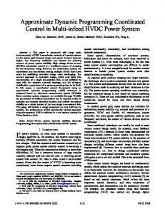
XII. PARTIAL SHAPERECOGNITION EXPERIMENTS For the partial shape recognition experiments, libraries with 143 views of each of six classes of aircraft were used, similar to the data used by Dudani [4].For each class of aircraft, 50 unknown views were generated. Both the known and unknown contours were generated at an image resolution of 128 X 128. To create partial shapes, the unknown contours were chopped, with the chopped portions being replaced by a straight line, a 90" turn, and another straight line. Contours were chopped by 10, 20, 30, 40, and 50 percent. These are much like the contours used by Davallou [19]. Some sample contours are shown in Fig. 19. Fig. 19(a) shows contours from four different aircraft, each at a different orientation. In Fig 19(b) and (c), these contours are shown after chopping by 20 and 40 percent, respectively. Fig. 20 shows a typical problem which is encountered when attempting to identify unknown partial aircraft contours. In Fig. 20(a), the unknown contour is shown. An incorrectly matched contour is shown in Fig. 20(b), and the correctly matching contour is shown in Fig. 20(c). Even a human observer might be hard pressed to make the correct choice without the help of additional information. Each unknown contour was compared to all of the library contours to find the best match. The library contour with the least distance from the unknown contour was taken to be the best match. If the best matching library contour belonged to the same library as the unknown contour, then the classification was considered to be correct. This experimental procedure meant that for each of the six difference chopping percentages, each of the 300 unknowns were tested against all 858 known contours (6 libraries of 143 views each).

(C) Fig. 19. Sample unknown contours: (a) unchopped, (b) chopped by 20 percent, and (c) chopped by 40 percent.

U U (C) Fig. 20. Classification error example: (a) unknown contour, (b) incorrect match, and (c) correct match.

Experiments were performed using the dynamic programming algorithm in its raw form without enhancements, and also with distance table clipping, the size constraint, and the partial shape weighting all being used. The purpose was to show the power of the algorithm in its raw form and the increase in performance derived from the enhancements to the algorithm. This algorithm was also used to classify contours which suffered

T

266

IEEE TRANSACTIONS ON PATTERN ANALYSIS AND MACHINE INTELLIGENCE, VOL. IO, NO. 2. MARCH 1988

TABLE I1 COMPARlSflN OF RAWALGORITHM TO ENHANCED ALGORITHM Comparison of Raw to Enhanced Algorithm Classification Accuracy enhanced algorithm algorithm

percent contour chopped

Classification accuracy for contours which were chopped in two places is shown in Table IV. It should be noted that the performance for the cases with two 5 percent chops and two 10 percent chops is only slightly worse than that for a single chop of the size of the sum of the two. This demonstrates that the algorithm can handle two distortions almost as easily as it can one distortion, making it useful for a wide variety of shape distortion problems.

89.33

93.00

XIV. CONCLUSIONS

10.0

78.33

82.33

A technique for recognition of partially distorted or incomplete

20.0

73.67

75.00

30.0

64.33

71.67

40.0

54.33

64.67

50.0

42.33

51.67

contours has been described. Local features were obtained from Fourier descriptors of contour segments, and a matching technique using dynamic programming was formulated. Criteria for evaluation of match quality were discussed, and partial shape recognition experiments were conducted. This technique has been shown to recognize unknown contours which have been rotated and translated, and which may be occluded or may overlap other objects. The unknowns may appear at any orientation with respect to the camera, and precise knowledge of scale is not required. Results indicate that partial contours can be recognized with reasonable accuracy.

percent contour chopped

Classification Accuracy segment full matching contour method method

0.0

93.00

92.00

10.0

82.33

83.67

20.0

75.00

58.00

71.67

30.33

64.67

22.00

51.67

12.67

TABLE IV PERFORMANCE WITH Two CHOPPED SECTIONS PER CONTOUR

20.0

71.67

30.0

60.00

40.0

55.67

50.0

47.33

distortion at two locations. Random locations were chosen for the starting points of each chop, and unknowns were generated for contours with two 5, 10, 15, 20, and 25 percent chops. XIII. EXPERIMENTAL RESULTS The experimental results are summarized in Tables 11-IV. Table I1 shows a comparison of the performance of the raw dynamic programming algorithm to that of the algorithm with the enhancements. The raw algorithm performs reasonably well, but one can see that the use of clipping, the size constraint, and partial shape weighting lead to significant improvements, especially as more of the contour is chopped. In Table 111, the performance of the segment matching method is compared to a method which uses Fourier descriptors of the entire boundary 131. While the segment matching method is slightly inferior when the contours are slightly chopped, it is clear that as more of the contour is chopped, the segment matching technique shows greatly improved performance over the method which uses the entire boundary.

REFERENCES [ I ] T. P. Wallace and P. A. Wintz, “An efficient three-dimensional aircraft recognition algorithm using Fourier descriptors,” Cornput. Graphics Image Processing, vol. 13, pp. 99-126, 1980.

[2] C. T. Zahn and R. Z. Roskies, “Fourier descriptors for plane closed curves,” IEEE Trans. Cornput., vol. C-21, pp. 269-281, Mar. 1972. 131 T. A. Grogan and 0. R. Mitchell, “Shape recognition and description: A comparative study,” School Elec. Eng.. Purdue Univ., West Lafayette, IN, Tech. Rep. TR-EE 83-22, 1983. [4] S . A. Dudani, “Aircraft identification by moment invariants,” lEEE Trans. Compur., vol. C-26, pp. 39-46, Jan. 1977. [5] M. K. Hu, ‘‘Visual pattern recognition by moment invariants,’’ IEEE Trans. Inform. Theory, vol. IT-8, pp. 179-187, Feb. 1962. [6] I . W. McKee and J. K. Aggarwal, “Computer recognition of partial views of curved objects,” IEEE Trans. Cornput., vol. C-26, pp. 790800, Aug. 1977. [7] W. A. Perkins, “A model-based vision system for industrial parts,” IEEE Trans. Compur, vol. C-27, pp. 126-143, Feb. 1978. 181 R. C . Bolles and R. A. Cain, “Recognizing and locating partially visible objects: The local-feature-focus method,” Inr. J . Robotics Res., vol. I , pp. 57-82, Fall 1982. [9] D. H. Ballard, “Generalizing the Hough transform to detect arbitrary shapes,” Pattern Recognition, vol. 13, no. 2, pp. 111-122, 1981. 1101 U. Ramer, “An iterative procedure for the polygonal approximation of plane closed Curves,” Compur. Graphics Image Processing, vol. I , pp. 244-256, 1972. [ l l ] R. Bellman and S . Dreyfus, Applied Dynamic Programming. Princeton, NJ: Princeton Univ. Press, 1962. [12] S . E. Dreyfus and A. M. Law, The Art and Theory of Dynamic Programming. New York: Academic, 1977. [I31 D. Sankoff and J . B. Kruskal, Eds., Time Warps, String Edits, and Macromolecules: The Theory and Practice of Sequence Comparison.

Reading, MA: Addison-Wesley, 1983. [I41 H. Sakoe and S . Chiba, “Dynamic programming algorithm optimization for spoken word recognition.” IEEE Trans. Acousr., Speech, Signal Processing, vol. ASSP-26, Feb. 1978. 1151 C. M. Myers, L. R. Rabiner, and A. E. Rosenberg. “Performance tradeoff in dynamic time warping algorithms for isolated word recognition,” IEEE Trans. Acoust., Speech, Signal Processing, vol. ASSP-28, Dec. 1980. 1161 J. O’Rourke and R. Washington, “Curve similarity via signatures,” in Computational Geometry. Amsterdam: Elsevier Science, NorthHolland, 1985, pp. 295-317. [I71 H. Fuchs, Z . M. Kedem, and S. P. Uselton, “Optimal surface reconstruction from planar contours,” Commun. ACM, vol. 20, Oct. 1977. [IS] J . P. Gifford, “Classification of three-dimensional partial shape using local descriptors,” Master’s thesis, Purdue Univ., West Lafayette, IN, May 1982. 1191 F. Davallou, 0. R. Mitchell, and F. P. Kuhl, “Recognition of partially-distorted contours using local features,” presented at the 1984 Conf. Intell. Syst. Machines, Rochester, MI, Apr. 1984.