May 6, 2002 - its preferred pattern and binarizes the neural code. ... The neural code thus becomes binary, and ..... Series, IOS Press, Amsterdam. pp.
To appear in Biosystems 2002
Synaptic depression increases the selectivity of a neuron to its preferred pattern and binarizes the neural code. Guido Bugmann Institute of Neuroscience and Centre for Neural and Adaptive Systems School of Computing, University of Plymouth, Plymouth PL4 8AA, United Kingdom http://www.tech.plym.ac.uk/soc/staff/guidbugm/ 5/6/2002 12:48 Abstract: The preferred pattern of a neuron consists here of the set of feature detectors from which it receives excitatory inputs. It is shown that the Leaky Integrate-and-Fire (LIF) model of a neuron has a poor selectivity to its preferred pattern. Its response is determined by the total current injected by input spike trains. Thus, a few inputs with a high activity (an incomplete pattern) can elicit the same response as many inputs (a complete pattern) with a weak activity. A theoretical model of depressing synapse with linear recovery is proposed which eliminates this problem. Using this model, the time-averaged current injected in the soma by a spike train becomes independent on its frequency. The neural code thus becomes binary, and the response strength of the target neuron depends only on the number of active inputs. Simulations show that a biological model of strong synaptic depression has effects similar to those of the ideal linear model. The best selectivity is obtained with long somatic decay time constants (> 50ms) and with depression recovery time constants larger or equal to the somatic decay time constant. Thus, by eliminating information carried in the input firing rate, a neuron can improve its pattern recognition performance. Keywords: Pattern recognition, Neuronal coding, Neuron model, Hamming distance. 1. Introduction Synaptic transmission in most neurons shows either short-term depression or potentiation. In the primary visual cortex (V1), potentiation is mainly seen in synapses involved in the local intracortical network dynamics, while depression is more often associated with thalamocortical inputs involved in pattern recognition (Gil et al., 1997). We focus here on the possible role of synaptic depression in pattern recognition. In recent years, synaptic depression has attracted the attention of many modelers who mainly focused on the dynamic implications of the phenomena. This include the time course of post stimulus time histograms (PSTH) in V1 (Muller et al, 2001), cross-orientation suppression (Carandini et al., 2001), the resolution-integration paradox in auditory processing (Denham, 2001), detection of synchronous inputs (Senn et al, 1998), temporal filtering of signals in electric fish (Rose and Fortune, 1999), invariant detection of firing rate transients (Abbott et al, 1997), and many others. Of special interest however is a model of the layer 4 circuitry in V1 (Kayser et al., 2001) which can simultaneously account for several contrastdependent non-linearities in cortical responses. In particular, the authors note that synaptic depression contributes to solving the problem of contrast-invariant orientation tuning. In this paper, synaptic depression is introduced as a theoretical solution to a related problem, that of the poor selectivity of the LIF neuron model when used as a pattern recognizer. A strong case has been made by Barlow (2001) that the brain should use a sparse rather than a distributed representation. This requires that as few as possible neurons respond when a given stimulus is presented. Hence, it is important that a neuron responds very selectively to the presentation of its preferred pattern. In section 2, the concepts of pattern recognition and selectivity are clarified, and the modest performance of an LIF neuron as a pattern recognizer is illustrated. We consider here patterns represented only by excitatory inputs, where each input represents one of the features from which the preferred
1
To appear in Biosystems 2002
pattern is constructed. In (Miller et al., 2001) it is proposed that a push-pull combination of feed-forward excitation and inhibition maybe be a more biologically realistic scheme. In the push-pull concept, additional inhibitory inputs may be used to reduce the total input current when some of the features of the presented pattern do not correspond to features of the preferred pattern. This improves the selectivity but, assuming that the preferred pattern of any neuron occurs infrequently in a natural environment, this scheme would lead to an almost permanent high inhibitory activity in the cortex. This defeats one of the original purpose of a high selectivity, which is the reduction of total energy consumption (Barlow, 2001). Thus, we focus here on how to achieve a high selectivity using excitatory inputs only. In section 3, an ideal model of synaptic depression with linear recovery is proposed to improve the selectivity. This is achieved by weakening the effect of inputs with a high activity. In section 4 it is proposed that biological synaptic depression should have a similar effect than the linear model. Simulations show that a significant improvement in selectivity can be achieved by using the biological model. A strong form of synaptic depression is used here, where the synaptic efficacy is reset to zero after each input spike and recovers exponentially (Bugmann, 1992). In section 5, the implications of synaptic depression for neural coding are discussed. It is proposed that synaptic depression generates a binary neural code, where the only relevant information is the active or inactive state of the input neurons. This produces a neuron that encodes the similarity between the presented pattern and the preferred pattern in terms of Hamming distance. The conclusion follows in section 6. 2. Quality of pattern recognition using a Leaky Integrate-and-Fire neuron (LIF) Neurons are hardwired to a set of input neurons and act as recognizers for the pattern represented by the co-activity of these inputs. A classical example is the detection of oriented bars by neurons in area V1 of the visual cortex. The preference for bars of a given orientation is achieved by the alignment of the receptive fields of the input neurons to which V1 neurons are connected (Hubel and Wiesel, 1962). This principle is not necessarily restricted to visual patterns, and any set of inputs connected to a neuron can be considered to represent the preferred pattern of that neuron. In this paper we will use the shape “E” to represent this set (figure 1), and shapes obtained by removing parts of the "E" will represent cases where only a fraction of the neurons in the input set are active. This is for instance the case when a bar is presented with a non-preferred orientation. A key concept throughout this paper is that the preferred pattern is assumed to be present when all inputs are active. The strength of the activity of the inputs is not relevant as long as it exceeds a given threshold. For instance, in the top row of figure 2A, a low-contrast “E”, represented by inputs with a low activity, and a high-contrast “E” represented by inputs with a high activity should both be recognized as an “E”. However, when only a fraction of the input set is active, as exemplified in lower rows in figure 2A by “F”, “L”, “I” and “-“, then the preferred pattern is not present and should not be recognized, regardless of the activity of these inputs.
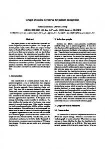
Figure 1. The LIF neuron used for pattern recognition. A complete pattern is represented by 50 input neurons firing Poisson spike trains with firing rates up to 100 Hz. A standard LIF neuron model is used, with EPSC's in the form of alpha functions and with partial reset of the somatic potential after an output spike. Simulation environment: CORTEXPRO.
2
To appear in Biosystems 2002
A standard LIF neuron model is used, in which each arriving spike generates an EPSC 1 2 represented by an alpha-function with Tmax = 1ms . The charges injected by input spikes are integrated in the capacitor C and are partly lost by leakage through the resistor R. The capacitance C is set to be C=1, which is equivalent to the rescaling of the synaptic efficacies. In that case, the resistance R is equal to the leakage time constant τRC. If the average input current exceeds the leakage current, the capacitor eventually reaches the firing threshold Vth = 15 mV and produces an output spike. The model keeps integrating input currents during the 3 refractory time Tr = 2ms. When a spike is produced, the potential undergoes partial reset, whereby it is reset to a reset voltage defined as a fraction β of the threshold: Vreset = βVth, where β== 0.91. Previous studies have shown that β== 0.91 leads to the production of spike trains with irregularities similar to those observed in cortical neurones (Bugmann et al, 1997). At the start of a simulation, the initial potential is the resting potential Vrest = 0. The time for producing the first spike is longer for smaller input currents, as can bee seen in figure 2B, where the input current was slightly reduced in each successive run. The lowest detectable contrast is arbitrarily defined as being represented by inputs firing at a rate of 20 Hz. This is above the background firing rate of most neurons. The maximum contrast is represented by inputs firing at 100Hz. To ensure the detection of complete patterns represented by 50 inputs firing at 20Hz, the synaptic weights are set such that the LIF neuron recognizes the input in approximately 95% of the runs. The recognition criterion used here is the production of at least one spike within 200 ms of stimulus presentation. This arbitrarily set time window corresponds approximately to the duration of fixation between saccades and can be considered as a reasonable maximum available recognition time. In this approach, observing the first spike gives us all the information we need, in accordance with recent information-theoretic analysis of experimental 4 data (Wiener and Richmond, 2001, Petersen et al., 2001) . To determine how good the LIF neuron is at recognizing its preferred pattern and at rejecting incomplete versions of it, we have run simulations where the number of inputs was progressively reduced from 50 to zero. The smallest number of active inputs required to produce a response was then noted. Figure 2B shows an example of spike trains produced during a simulation where the number of active inputs is reduced by one in each run. The numbers of necessary active inputs for various input firing rates are shown in figure 2A. These numbers are the same, within measurement errors, for membrane decay time constants τRC = 10ms, 20 ms, 50ms or 100ms. For each time constant, the synaptic weights Wij were re-adjusted to achieve the desired response probability of around 95% for inputs firing at 20Hz (all inputs had the same weight, i.e. for τRC = 10ms, 20 ms, 50ms and 100ms, the weights were respectively Wij = 0.45, 0.26, 0.12 and 0.075).
1
The alpha function is given by
EPSC ij (t ) =
t − t0 t − t0 exp(− + 1) , where t0 is the arrival Tmax,ij Tmax,ij
time of the spike. The “+1” in the exponential ensures that the maximum amplitude is 1, whatever the value of Tmax,ij. Tmax,ij is the time where the peak amplitude is reached. 2 . The total electric charge injected by one EPSC is the area under the alpha function, i.e. ∆Qij = exp(1)*Wij*Tmax,ij, where Wij is the synaptic weight. 3 This leads to a transfer function that stays linear over a larger range of input currents than the one obtained by interrupting the integration during the refractory time. 4 It is another question if a single spike can have a useful effect on a target neuron. We will see in the discussion that it would have been more consistent to require from the firing rate to be above some minimum rate, but both recognition criteria lead to the same conclusions. 3
To appear in Biosystems 2002
A
B
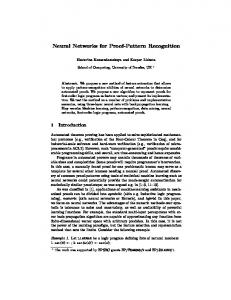
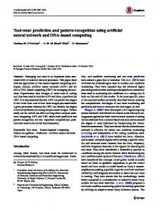
Figure 2. A: Performance of a LIF neuron as a pattern recognizer. (i) The symbols show the minimum number of active inputs needed for a given input firing rate, for different somatic decay time constants τRC (the symbol + corresponds to τRC =10 ms, ∆: 20 ms, X: 50 ms, square box: 100 ms). Synaptic weights are set so that the LIF neuron responds to 50 inputs firing at 20Hz in approximately 95% of the runs. A response consists of at least one spike fired within 200ms after stimulus presentation. The stimulus consists of Poisson inputs firing all at the same rate, starting at time 0. (ii) The dotted curve shows the points where the current injected by input spike trains is equal to the threshold current (equ. 1). (iii) The alphabetic characters are centered on the point corresponding to their number of active inputs and the level of activity of these inputs. For instance, the low-contrast "E" at the top left represents all 50 inputs firing at 20Hz, and the high-contrast "-" at the bottom right represents 10 inputs firing at 100Hz. B: Example of spike trains produced when the number of inputs is reduced by one in each run, from 50 at the bottom to zero at the top. All active inputs fired at 40 Hz. Figure 2A shows that the LIF neuron would respond to only 10 out of 50 inputs, providing that these fire with a high enough rate. This corresponds to recognizing a “-“ as an “E”. The cause 5 of this poor performance lies in the fact that the 50 inputs firing at 20 Hz have the same impact as 10 inputs firing at 100 Hz. This suggests that the LIF neuron acts essentially as a current detector over a wide range of membrane time constants. This is confirmed by the good match between the experimental points obtained from simulations such as the one shown in figure 2B, and the doted line in figure 2A. The line represents the points where the average current Iav injected by input spike trains is equal to the current threshold Ith.
I av ,i =
Nact j =1
f in , j ∆qij ≥ I th =
Vth R
(1)
Where Nact is the number of active inputs, ∆qij is the charge injected in the soma of neuron i by each spike from input j, and fin,j is the firing rate of input j.
5
The performance can be quantified using information theoretic methods, but for compactness, this is not presented here. 4
To appear in Biosystems 2002
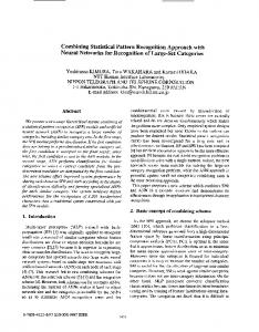
Figure 3. Firing rate or the LIF neuron in two conditions: (i) when the number of inputs is kept fixed (n =40) and the input firing rate is variable, or (ii) when the input frequency is fixed (fin = 80 Hz) and the number of active inputs is varied. Other parameters: Wij = 0.075, τRC = 100ms. The output firing rate fout of the LIF neuron is only determined by the average input current 6 injected by the Nact active inputs (figure 3) . Nact
f out ,i = S (
j =1
f in , j ∆qij )
(2)
where S() is a sigmoid squashing function. This function is similar to that of a formal neuron used in artificial neural networks:
yi = ϕ (
N j =1
y j wij )
(3) 7
Where yi is the output of formal neuron i , ϕ() is a sigmoid squashing function , and wij is the synaptic weight from formal neuron j to formal neuron i. An apparent solution to the problem of the poor selectivity of the LIF neuron is to increase its threshold Vth. However, this causes a shift of the decision curve in figure 2A towards the upper right corner and makes faint but valid patterns undetectable. The improvement to be sought is the rejection of incomplete patterns and the preservation of faint ones, i.e. a vertical compression of the decision curve in figure 2A. The LIF neuron model above is equivalent to the original Hubel and Wiesel (1962) model of orientation tuning in the primary visual cortex. This model performs linear summation of the activities of the inputs followed by a thresholding function. It is known that this model does not reproduce correctly the contrast invariance of the tuning curve (see e.g. Ferster and Miller, 2000). 3. Binarizing the neural code using a linear depressing synapse In this section we propose a theoretical solution to the low selectivity of the LIF neuron model illustrated in section 1. The idea is that, if an input firing at 100 Hz could be made no more potent than an input firing at 20Hz, then a few inputs firing at high rate would not be able to compensate for a number of silent inputs. Hence, the neuron would need all its inputs to fire and would be a more selective pattern recognizer. The approach proposed here is to design a time-dependent synaptic efficacy such that the input current carried by each spike train becomes independent on the firing rate of that spike train.
6
There is a more complex behaviour a very low output firing rates, where fluctuation detection plays a role, but this only concerns a small fraction of the input current range. 7 The functions ϕ and S differ mainly by a horizontal shift along the current axis. 5
To appear in Biosystems 2002
Figure 4. Linear model of synaptic depression. The synaptic efficacy is measured by the electric charge ∆qij,k injected by a spike arriving at time tk at synapse ij. Let us assume that the synaptic efficacy ∆qii,k is time-dependent, decreasing to zero after each input spike, and recovers linearly with time (figure 4):
∆qij (t k , t k −1 ) = ∆qij 0 ⋅ (t k − t k −1 )
(4)
The longer the time delay between two spikes, the larger the current ∆qij(tk,tk-1) injected by a spike into the target neuron. The mean current Iav,ij carried by a spike train from neuron j to i then becomes a constant:
I av ,ij =
1 T
T k =1
∆q jio ⋅ (t k − t k −1 ) = ∆qijo
(5)
Where T is an arbitrary long duration over which the spike trains is observed. Using this approach, the information carried in the firing rate of a spike train is discarded by the synapse of a target neuron. The only fact that counts is that the input neuron is active. This is a binary piece of information and the threshold of the target neuron now determines how many active inputs are required for firing. The model has an untidy behaviour when an input fires at a very low frequency, as each 8 spike then injects a huge charge in the neuron . However, this problem does not occur with the biological model below. 4. Improved selectivity using a biological model of depressing synapse In biological depressing synapses, the recovery curve is not linear, but depression could play a qualitatively similar binarizing role. We will determine here how much improvement in selectivity can be expected from biological depressing synapses.
8
This can be avoided in practice by setting a maximum synaptic efficacy, say for inputs firing below 20Hz (tk-tk-1 > 50ms). However, with Poisson inputs, this limit will also affect to some extent inputs firing at a higher rate. 6
To appear in Biosystems 2002
Figure 5. Theoretical model of strong synaptic depression. The synaptic efficacy is totally reset after each spike and recovers exponentially (equ. 6). Figure 5 illustrates the model used in our simulations. This is a strong form of depression where 100% of the synaptic efficacy lost after each spike (Bugmann, 1992). Values derived from experiments indicate losses of up to 95% (Tsodyks and Markram, 1997, Varela et al., 1997) or even 98% (Muller et al., 2001). Other pre- and post-synaptic effects also contribute to reducing the impact of high input firing rates. For instance, an increase of the rate of axonal conductance failures is often observed for short interspike intervals (see e.g. Stratford et al., 1996). Synaptic release failure also increases when the number of release sites is small, as modeled in Goldman et al (2002). For simplicity, we will assume here that all these effects can be subsumed into a strong depression model with a single exponential recovery curve.
∆qij (t k , t k −1 ) = ∆qij 0 ⋅ [1 − exp(−
t k − t k −1 )] τ rec
(6)
The average current injected in the soma by all spike trains is given by and integral over all possible interspike intervals weighted by their distribution in a Poisson spike train: ∞
I av = Nact ⋅ f in ⋅ ∆qij 0 ⋅ [1 − exp(− 0
t
τ rec
)] ⋅ f in exp(−t ⋅ f in ) ⋅ dt
(7)
resulting in: 2
I av = Nact ⋅ f in ∆qij 0 ⋅ (
τ rec 1 ) − f in 1 + f in ⋅ τ rec
(8)
Figure 6 show the improvement in performance that can be obtained with synaptic depression according to equation (6). The LIF neuron has become more selective, responding to the much smaller set of input patterns above the line defined by Iav = Ith.
7
To appear in Biosystems 2002
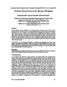
Figure 6. Pattern recognition performance of the LIF neuron with synaptic depression (τrec=100ms). The square symbols represents the minimum number of active inputs required at each input frequency. The full line represents the number of active inputs which inject the threshold current for a given input frequency, using equation (8). Figure 7 shows that the gain in selectivity due to synaptic depression is limited by the somatic decay time constant. When the depression recovery time constant is larger than the somatic decay time constant, there is no additional gain in selectivity. The selectivity is best with long leakage decay time constants and with recovery time constants matching it or longer. For τRC 9 ==τd = 100ms the performance of the biological model (equ. 6) is very close to the performance of the ideal linear model (equ. 4). In this balanced case, i.e. when both time constants are equal, synaptic depression stabilizes the amplitude of the potential increase due to the charge injected by each spike. This condition is ideal for detecting coincidences of inputs spikes (Bugmann, 1992). However, for a large number of inputs firing at rather low rates such as those considered in this paper, spike coincidences are exceedingly rare. Here the LIF neuron operates as a detector of co-active inputs in the sense that its firing indicates that a number of inputs are firing.
9
Somatic time constants of 10-30 ms are generally used in simulations and 100ms may seem an excessively large value. However, there is some debate about the downward bias introduced by measuring methods.
8
To appear in Biosystems 2002
Figure 7. Effect of the recovery time constant on the selectivity of the LIF neuron as pattern recognizer. The selectivity is measured here by the minimum number of inputs firing at 100 Hz required by the LIF neuron for various recovery time constants of the depressing synapse and somatic decay times τRC . This measure corresponds to the last point on the right of curves such as shown in figures 2A and 6. The higher this value, the more selective the LIF neuron. The dashed line is obtained from simulations of the ideal linear model of synaptic depression (eq. 4). The synaptic weights were set as in explained section 2 for each combination of τRC and τrec.
Figure 8. Output firing rate of the LIF neuron with depressing synapses (τrec=100ms) in dependence on the number of active inputs, for inputs with the indicated firing rates. Other parameters: τRC = 100 ms, Wij = 0.17. 5. Implications for the neural code Synaptic depression induces a shift of the neural code from rate-based to number-of-activeinputs-based. Without synaptic depression, the output firing rate of the neuron signals by how much the average input current is above the current threshold. The neuron behaves as a formal neuron, by bisecting the high-dimensional input space of firing rates. The number of active inputs that generate a given current is irrelevant. With synaptic depression, the output firing rate signals how many inputs are active, with very little dependence on how strongly the inputs fire, provided that the number of active 10 inputs is above a given threshold number (figure 8) . The number of active inputs can be used as a measure of the similarity between the presented pattern and the preferred pattern. Thus, the neuron makes a decision in the similarity space. Although similarity information is available in the output firing rate, this information would be discarded by the next neuron in a hierarchical network of neurons with synaptic depression, as these treat the firing rate as binary information. A logical 1 corresponds in our 10
This threshold defines a maximum allowed Hamming distance between the presented pattern and the preferred pattern. 9
To appear in Biosystems 2002
case to a firing rate above 20 Hz. Hence, it could be argued that the proper criteria for a response is not that the neuron produces a spike in a given time window (as in section 2), but that it fires with a rate above 20 Hz. Fortunately, both criteria turn out to be almost equivalent, as 50 active inputs firing at 20 Hz, produce an output frequency only slightly below 20 Hz (figure 8). There is no reason to exclude that both codes may be used in different parts of the biological neural network. However, the fact that synaptic depression seems to be required to explain a number of properties of the responses of V1 neurons, such as contrast invariance (Kayser et al., 2001 , see also figure 8), and time course of the PSTH (Muller et al., 2001), suggests that al least the visual system is taking advantage of the benefits of synaptic depression in its pattern recognition tasks. 6. Conclusion The model of strong synaptic depression used here is assumed to be a compact representation of several experimentally observed effects that combine to reduce the impact of high frequency input spike trains. The validity of this simplification remains to be verified. Another issue is the fact that synaptic depression is most effective here with long somatic decay time constants (>50ms). In many neurons, these may not be as long. However, even with weaker depression and shorter decay time constants, the trends indicated by the results in this paper are expected to remain valid. Namely, synaptic depression improves the performance of a LIF neuron in a pattern-recognition task. This is achieved by binarizing the neural code. Therefore, a rather counterintuitive conclusion is that by discarding information carried in the firing rates, neurons can achieve a better pattern recognition performance. Acknowledgments The author is grateful for fruitful discussion with Roman Borisyuk, Jochen Braun, Sue Denham and Roddy Williamson. Technical support by Dave Stevens is acknowledged. References Abbott L.F., Varela J.A., Sen K., and Nelson S. B. (1997) “Synaptic depression and cortical gain control” Science, 275, pp. 220-224. Barlow H.B. (2001) “Redundancy reduction revisited”. Network : computation in neural systems 12, pp. 241-253. Bugmann, G. (1992) "Multiplying with neurons: Compensation for irregular input spike trains by using time dependent synaptic efficiencies" Biological Cybernetics, 68, pp. 87-92. Bugmann G., Christodoulou C. and Taylor J.G. (1997) "Role of Temporal Integration and Fluctuation Detection in the highly irregular firing of a Leaky Integrator Neuron Model with Partial Reset" Neural Computation, 9, pp. 985-1000. Carandini M., Heeger D.J. and Senn W. (2001) “Cross-Orientation suppression in V1 explained by synaptic depression”, Soc. Neurosci. Abstr., Vol. 27, Program No 12.12. Denham S. L. (2001) “Cortical synaptic depression and auditory perception”. In: Computational Models of Auditory Function”, Greenberg S. and Slaney M. (eds), NATO ASI Series, IOS Press, Amsterdam. pp. 281-296. Ferster, D. and Miller, K.D. (2000) Neural mechanisms of orientation selectivity in the visual cortex. Annual Reviews of Neuroscience 23, pp. 441-471. Gil Z., Connors B.W. and Amitai Y. (1997) “Differential regulation of neocortical synapses by neuromodulator and activity”, Neuron, 19, participants. 679-686.
10
To appear in Biosystems 2002
Goldman M., Maldonado P., Abbott L.F. (2002) “Redundancy reduction and sustained firing with stochastic depressing synapses” J. Neuroscience, 22, pp. 584-591. Hubel D.H. and Wiesel T.N. (1962) “Receptive fields, binocular interaction and functional architecture in the cat's visual cortex.”, J. Physiol., 160, pp.106-154. Kayser, A., Priebe N.J. and Miller K.D. (2001). “Contrast-dependent nonlinearities arise locally in a model of contrast-invariant orientation tuning”. Journal of Neurophysiology, 85, 21302149. Miller K.D., Pinto D.J. and Simons D.J. (2001) "Processing in layer 4 of the neocortical circuit: new insights from visual and somatosensory cortex", Current Opinion in Neurobiology, 11, pp. 488-497. Muller J.R., Metha A.B., Krauskopf J. and Lennie P. (2001) "Information conveyed by onset transients in responses of striate cortical neurons" J. Neuroscience, 21:17, pp. 6978-6990. Petersen R.S., Panzeri S. and Diamond M.E. (2002) "The role of individual spikes and spike patterns in population coding of stimulus location in rat somatosensory cortex", Biosystems, -- this issue ----Senn W., Segev I. And Tsodyks M. (1998) “Reading neuronal synchrony with depressing synapses” Neural Computation, 10, pp. 815-819. Stratford K.J., Tarczy-Hornoch K., Martin K.A., Bannister N.J. and Jack J.J.B. (1996) “Excitatory synaptic inputs to spiny stellate cells in the cat visual cortex”, Nature, 382, participants. 258-261. Tsodyks, M. & Markram, H. (1997) “The neural code between neocortical pyramidal neurons depends on neurotransmitter release probability” Proceedings of the National Academy of Sciences of the USA, 94; 719-723. Varela J., Sen K., Gibson J., Fost J., Abbott L.F. and Nelson S.B. (1997) “A quantitative description of short-term plasticity at excitatory synapses in layer 2/3 of rat primary visual cortex” J. Neuroscience, 17, pp. 7926-7940. Wiener M.C. and Richmond B.J.(2002) "Model based decoding of spike trains", Biosystems, -- this issue ---
-------------size--------------Abstract = 201 words Main text = 3689 19 References = 19 x 21 = 399 9 figures on 1 column x 5 cm = 80 x 9 = 720 words Total without abstract: 4808 (4406-201-516=3689)
11