John S. Hollywood. S.B. Applied Mathematics ... Production at any station depends on work-in-queue levels through some production function. (5) We can.
Performance Evaluation and Optimization Models for Processing Networks with Queue-Dependent Production Quantities by John S. Hollywood S.B. Applied Mathematics Massachusetts Institute of Technology, 1996 Submitted to the Department of Electrical Engineering and Computer Science in Partial Fulfillment of the Requirements for the Degree of Doctor of Philosophy in Operations Research at the Massachusetts Institute of Technology June 2000 © 2000 Massachusetts Institute of Technology All rights reserved
Signature of Author . . . . . . . . . . . . . . . . . . . . . . . . . . . . . . . . . . . . . . . . . . . . . . . . . . . . . . . . . . . . . . . . . . . . Department of Electrical Engineering and Computer Science May 5, 2000
Certified by . . . . . . . . . . . . . . . . . . . . . . . . . . . . . . . . . . . . . . . . . . . . . . . . . . . . . . . . . . . . . . . . . . . . . . . . . . . Stephen C. Graves Abraham J. Siegel Professor of Management and Co-Director, Leaders for Manufacturing Thesis Supervisor
Accepted by . . . . . . . . . . . . . . . . . . . . . . . . . . . . . . . . . . . . . . . . . . . . . . . . . . . . . . . . . . . . . . . . . . . . . . . . . . . Cynthia Barnhart Associate Professor of Civil Engineering Co-Director, MIT Operations Research Center
1
Performance Evaluation and Optimization Models for Processing Networks with Queue-Dependent Production Quantities by John S. Hollywood Submitted to the Department of Electrical Engineering and Computer Science on May 5, 2000 in Partial Fulfillment of the Requirements for the Degree of Doctor of Philosophy in Operations Research
Abstract We consider a class of models for processing networks such as job shops or distributing data-processing systems. The defining features of this class of models are: (1) The network operates in discrete time, such that work is completed during fixed-length periods and work arrivals and transfers occur at the start of these periods. (2) Work arrivals are stochastic, characterized by a finite mean and variance. (3) Work flows are Markovian in that processing requirements do not depend on how the work got to a station. (4) Production at any station depends on work-in-queue levels through some production function. (5) We can write recursion equations (either exact or approximate) relating the moments of production and queue lengths in one period to the moments of production and queue lengths in the next period. We call models satisfying these properties Moment-Recursion (MR) models. MR models support a variety of performance evaluation, optimization, and decision-support applications, such as capacity planning, resource allocation, production smoothing, and inventory control. They apply to a wide range of scenarios in which production depends on work-in-queue levels. Most directly, MR models apply to shops with control rules that minimize production fluctuation, or with machines that show saturation effects. They apply to systems in which people work at varying speeds in response to work-in-queue levels, or show the effects of overtime. MR models also address networks in which resources may be reallocated between different flows of jobs at regular intervals, such as in flexible job shops or dataprocessing networks. We consider a variety of MR models, using the recursion equations to calculate the steady-state moments of the stations’ productions and queue lengths for all model types. These types include: • Models whose production functions are linear functions of the queue levels. These models may address basestock job shops, Kanban shops, and shops using other linear rules to minimize production variances. • Models with nonlinear production functions. We develop approximations for the steady-state moments using Taylor-series expansions of the production functions. • Models that maintain a constant weighted-inventory constraint. We use the resulting models to find weighted-inventory rules that minimize steady-state production fluctuations. • Models that incorporate complex work transfer relationships. Here, work completed upstream is converted into jobs (or lots), and then triggers job arrivals downstream through complex probabilistic relationships. We use the production and queue-length moments to solve a variety of steady-state optimization problems. We formulate maximum performance, maximum throughput, and minimum cost problems, and discuss nonlinear programming techniques to solve them. Finally, we use the recursion equations to describe the transient behavior of MR-networks. We first derive the exact transient moments for models with linear control rules, both analytically and numerically. We then derive the production functions that minimize quadratic objective functions of the production and queue-length quantities, and find that the optimal functions are always linear control rules. Thesis Supervisor: Stephen C. Graves Title: Abraham J. Siegel Professor of Management and Co-Director, Leaders for Manufacturing 2
Acknowledgements Eight years is a long time in college, especially at the Massachvsetts Institvte of Technology. My undergraduate house, Epsilon Theta, was a big part of my getting through it. Special thanks goes out to my pledge class, PC '92, along with "Uncle" Matt Condell, Alyse Leung, David Leung, and my nocturnalbut-great roommate, Jason Gratt. I would like to thank all of my colleagues and friends who I know through student activism, as well. Not just have they done incredible work for MIT for no reason other than their desires to help students, they have provided me with great friendship and support. Luis Ortiz, Matt McGann, Jen Berk, Jen Frank, Chris Rezek, Sarah McDougal, Shawn Kelly, Will Dichtel, Liana Lareau, Chris Beland -- this is for you. Special recognition goes out to best compadres Jeremy Sher and Jake Parrott, who made being one of the "3J's" far more than part of a poker hand or group of student-life advocates. How can I ever forget the last-minute gourmet meals and dinner trips? Also deserving of thank-yous are the student life administrators who set me on my stressful but rewarding student-activist path, notably Andy Eisenmann, Steve Immerman, "Uncle" Phil Walsh, Margaret Bates, and Mary Rowe. This is not to say that the Operations Research Center does not deserve my gratitude as well. My colleagues have done much to reinforce the ORC’s claim of being the best and friendliest place at MIT. I would especially like to thank my ORC cohort, CPT(P) Andy Armacost, Amy Cohn, Ozie Ergun, Jeremie Gallien, Martin Haugh, Brett Leida, and Marina Zaretsky. I would also like to express my appreciation for the professors who did so much to teach me OR and management, including Tom Magnanti, Jim Orlin, Dimitris Bertsimas, Larry Wein, Jack Rockart, and Starling Hunter, as well as my academic advisor, Dick Larson. Of course, there are my undergraduate professors, too, who did much to me during my first four years at MIT. Best wishes especially to Martha Weinberg, Charles Stewart, Steve Meyer, and Jon Lendon. Most of all, I would like to express my gratitude to Al Drake, who did so much to confirm my desire to go into Operations Research, both as my freshman advisor and then throughout my undergraduate career. I would like to thank Steve Graves, my advisor, for putting me on this interesting and important research path. More importantly, though, I would like to thank him for the great support and encouragement he has given me for the past four years. I also thank him for all the Operations Research and professional wisdom he has given me, through our meetings and seminars together. Finally, and most importantly, I would like to thank my family for their incredible love and support. In particular, I would like to recognize my grandparents and the love they gave me – I only wish I had more time with them. Most of all, I would like to thank my parents for the love and support they have given me over the years. They have always been there for me, for which I am forever grateful. This thesis is dedicated to them.
3
Contents Chapter 1: Introduction .......................................................................................................................6 1.
The Concept of a Moment-Recursion Model .............................................................................7
2.
Thesis Outline .........................................................................................................................9
3.
Literature Review..................................................................................................................14
Chapter 2: The Tactical Planning Model and Other Models with Linear Control Rules (Class LLS-MR) 19 1.
Introduction ..........................................................................................................................20
2.
The Tactical Planning Model..................................................................................................20
3.
The Tactical Planning Model for Pull-Based Systems ..............................................................30
4.
The General LLS-MR Model..................................................................................................32
5.
Example: A Stochastic Production System Using Proportional Restoration Control Rules ..........35
6.
Example: A Communications Problem....................................................................................38
Chapter 3: Models with General Control Rules (Class GLS-MR).........................................................52 1.
Introduction ..........................................................................................................................53
2.
The Delta Method for Production and Queue Length Moments.................................................56
3.
Steady-State Analysis for Models with Single -Queue Control Rules .........................................60
4.
Empirical Behavior of Models with Single -Queue Control Rules ..............................................71
5.
Steady-State Analysis for Models with Multi-Queue Control Rules...........................................85
6.
An Asymptotic Lower Bound on Expected Queue Lengths.......................................................91
Chapter 4: Models That Maintain a Constant Inventory (Class LLC-MR).............................................96 1.
Introduction ..........................................................................................................................97
2.
Review of the Tactical Planning Model...................................................................................97
3.
The Constant Inventory Model ...............................................................................................99
4.
Setting the Vector of Inventory Weights and the Initial Inventories......................................... 105
5.
An Example ........................................................................................................................ 111
Chapter 5: Models That Process Discrete Jobs (Class LRS-MR)........................................................ 116 1.
Introduction ........................................................................................................................ 118
2.
An Overview of the Model Development .............................................................................. 119
3.
An Example Job Shop.......................................................................................................... 132
4.
Discussion of the Model....................................................................................................... 138
5.
The Derivation of the LRS-MR model .................................................................................. 141
6.
Appendix: Lemmas Used in Model Derivations .................................................................... 175
4
Chapter 6: Steady-State Optimization............................................................................................... 183 1.
Introduction ........................................................................................................................ 184
2.
Formulation of Station Capacities ......................................................................................... 185
3.
General Forms of Optimization Problems .............................................................................. 196
4.
Nonlinear Programming Techniques ..................................................................................... 202
5.
Optimization of LRS-MR Models ......................................................................................... 206
6.
A Performance Measure: Expected End-to-End Completion Times......................................... 209
7.
Examples of MR-Model Optimization Problems .................................................................... 211
Chapter 7: Transient Analysis and Optimization of Models with Linear Control Rules ........................ 222 1.
Introduction ........................................................................................................................ 223
2.
Transient Analysis of Simple Changes to LLS-MR Models .................................................... 225
3.
Numerical Analysis of the Transient Behavior of LLS-MR Models ......................................... 231
4.
Optimal Control of MR Models ............................................................................................ 236
Chapter 8: Conclusions ................................................................................................................... 245 1.
Contributions ...................................................................................................................... 246
2.
Opportunities for Future Research........................................................................................ 247
References ..................................................................................................................................... 251
5
Chapter 1: Introduction
1.
The Concept of a Moment-Recursion Model.................................................................................7
2.
Thesis Outline .............................................................................................................................9
3.
Literature Review......................................................................................................................14
6
Chapter 1: Introduction
1. The Concept of a Moment-Recursion Model This thesis is devoted to studying the ramifications of a simple recursion equation, derived below. Consider a job shop or other network of processing stations. We model the shop in discrete time, such that stations process some amount of work in process during each time period, and transfer work to other stations (or out of the shop) at the start of the next time period. We also assume that work at a station can be modeled as a fluid (e.g. “3 hours of work at station 2”) rather than as a set of distinct jobs. Then, each station i must satisfy the following elementary inventory balance equation, Qi, t = Qi,t −1 − Pi,t −1 + Ait ,
(1)
where Qit is the queue level at the start of period t, Pi,t -1 is the amount of work processed over period t-1, and Ait is the amount of work that enters station i at the start of period t. We write the above inventory balance equations for all stations simultaneously in matrix form as: Q t = Q t−1 − Pt −1 + A t ,
(2)
where Qt is a vector of queue lengths, Pt is a vector of production quantities, and At is a vector of work arrivals. Suppose we make the following assumptions about Pt-1 and At. •
Pt-1 will be a function of the work in process at the start of period t-1. Then Pt−1 = p t −1 (Q t−1 ) , where p(⋅) is a production function or control rule. Note that Pt-1 usually is a deterministic function of Qt-1 ,
although we will consider situations where Pt is a probabilistic function. •
At has two components. The first consists of work sent from stations to other stations, and will be a probabilistic function of Pt-1 . This component incorporates the concept that completed work at one station triggers work at another station.
Mathematically, this component is ANt [P(Qt −1 )] , where
ANt [⋅] is the internal arrival function.
•
The second component of At consists of work that arrives to stations from outside the shop. We will also allow this component to depend on Qt-1 ; modeling the component this way will allow us to explore various control schemes such as constant inventory (or CONWIP) job shops. Mathematically, this component is ARt [Q t−1 ] , where ARt [⋅] is the external arrival function.
Now, substitute the above expressions for Pt-1 and At into the inventory balance equation. This yields the recursion equation that forms the basis of the thesis.
7
Chapter 1: Introduction (MR) Q t = Q t−1 − Pt −1 (Q t −1 ) + A Nt [P(Qt −1 )] + ARt [Qt −1 ]
(3)
At first glance, this equation does not appear useful since Qt is a random vector, and the various functions in the equation are probabilistic functions. However, suppose that the following conditions are satisfied: •
We know the expectation and variance of Qt-1 . (Note that E[Qt-1 ] is a vector and Var[Qt-1 ] is a covariance matrix).
•
We can use (3) to write closed-form expressions for E[Qt] and Var[Qt] in terms of E[Qt-1 ] and Var[Qt-1 ]. These expressions may be exact or approximate, depending on the production and arrival functional forms.
Call shop models that satisfy these two conditions moment-recursion (MR) models. We may generate exact or approximate estimates of E[Qt] and Var[Qt] for moment-recursion models. This fact is extremely useful. By repeatedly iterating our closed-form expressions for E[Qt] and Var[Qt], we can track the distributions of the shop queues over time. Similarly, by using the inventory balance equation, we can write variants of (3) in terms of the production moments, E[Pt] and Var[Pt]. Then we can track the distributions of the production quantities over time, as well. Alternately, assume we have a job shop that has a defined steady state (all stations in the shop are stable, aperiodic, and ergodic). Then we can iterate the closed-form expressions indefinitely, converging to steady-state values for E[Q] and Var[Q]. In some cases, we find closed-form expressions for E[Q] and Var[Q]; in other cases, we start with reasonable estimates for E[Q] and Var[Q] and converge to steadystate values. Similarly, we find steady-state values for E[P] and Var[P]. In many cases, these moments will be exact; in other cases these moments will be approximate, but quite accurate over the range of reasonably well-behaved networks.
Importantly, we will find that the steady-state moments are
3
calculated in O(n ) time, where n is the number of stations in the network. We may use the expected queue lengths to calculate the expected waiting times, E[W], as well. The thesis will show that there is a fast way to calculate the expected steady-state arrival rates at all stations using (3); then, by using Little’s Law, knowing E[Q] immediately yields E[W]. Knowledge of the moments of production and queue lengths are sufficient to carry out a great number of performance evaluation, optimization, and decision-support tasks. For example, we may use MR models to help optimize networks. We may maximize the performance of a network (as measured by waiting times or inventory levels), minimize the cost of the network (in terms of capacity costs), and maximize the expected throughput of the network. We may also find control policies that reduce production and queue length fluctuations (i.e., minimize the variances) – important in situations requiring output predictability such as Just-in-time manufacturing.
8
We may use a MR-model for “what-if”
Chapter 1: Introduction analysis, asking what will happen if a station is added, or work is re-routed, and receiving comprehensive results in terms of the production and queue-length moments (both transient and steady-state). We expect that MR-models will be applicable to the wide range of scenarios in which work is best treated as flows of jobs, and in which production quantities are related to queue levels. Examples of such scenarios include the wide range of environments in which people naturally work faster when more work is present, and slower when less work is present. Similarly, MR models apply to shops in which people work overtime; overtime work is less efficient than regular work, resulting in functional relationships between overtime work-in-queue and overtime production. Concerning machines, MR models apply to workstations showing saturating behavior (i.e. the machine’s work-per-period is flexible, but marginal work decreases with the work-in-queue). They also model flexible job shops, in which some resources may be moved around the shop between work periods, and in which stations support sophisticated production-control policies. Finally, MR models may be used in flexible data-processing environments, in which computing resources may be regularly reallocated between job processes. They also apply to computers that process multiple jobs simultaneously. Jobs are generally time-shared, so that an increase in jobs initially results in a direct increase in production. As more jobs are added, the computer becomes overloaded, so that the marginal increase in production declines with more jobs. Consequently, this thesis studies a variety of situations in which we can generate momentrecursion models. It also discusses optimization and decision-support applications for these models.
2. Thesis Outline This thesis presents steady-state analysis results for a variety of MR model classes, discusses steady-state optimization of MR models, and describes the transient analysis and control of MR models. To describe the models and applications presented in this thesis, we present a classification scheme for momentrecursion models. The scheme describes MR models as xxx-MR, where, xxx is a 3-letter prefix, and: •
The first letter describes the control rule function that determines how much of the work-in-queue to process each time period.
•
The second letter describes the work transfers between stations.
•
The third letter describes the work that enters from outside of the shop.
We have the following definitions for the letters in the classification scheme. •
Lxx-MR. The control rule is a linear function of the work-in-queue. Usually, we assume that the production rule is Pi = α iQi , where α i is a fixed constant in [0,1]. This rule states that stations 9
Chapter 1: Introduction process a fixed fraction of their work-in-queue each time period. We also consider the multi-queue linear control rule Pi = ∑ j α ijQ j ; this rule sets production to be a weighted sum of inventory levels throughout the network. •
Gxx-MR. The control rule is a general function of Qt, which we assume is continuous and twicedifferentiable. We will consider single -queue control rules and multi-queue control rules.
•
xLx-MR. The internal arrival function has the form ANt [Pt (Qt )] = F Pt−1 + e t . In other words, work arriving to a station is a linear combination of work at other stations plus random noise from an independent distribution.
•
xGx-MR. The internal arrival function is a general probabilistic function. (We will not consider xGx-MR models explicitly in this thesis.)
•
xRx-MR. The request-based external arrival function is a special type of function. It dictates that completed jobs, rather than completed work, generate work at downstream stations. In particular, the request-based function first divides completed work into some number of completed jobs. Completed jobs then become work requests at downstream stations. Each request generates a random number of jobs, and each job requires a random number of instructions to complete. The total number of instructions in queue at a station is the “work-in-queue” at the station.
•
xxS-MR. Arrivals from outside the shop come from an independent distribution.
•
xxL-MR. Arrivals from outside the shop depend linearly on Qt, e.g. AR t = BQt, where B is a matrix.
•
xxC-MR. A special subclass of xxL-MR, the external arrival function for this class generates new work to maintain a constant inventory constraint on the job shop. (We will restrict our consideration of xxL-MR models to this subclass.)
•
xxG-MR. Arrivals from outside the shop come from a stochastic function that depends upon Qt. (We will not consider xxG-MR models explicitly in this thesis.)
In Chapters 2-5, we explicitly consider the following MR models: Chapter 2: LLS-MR Models. (Linear control rules, linear internal arrival functions, and stationary external arrival functions.) LLS-MR models are the simplest class of MR models. Nonetheless, these models may be applied in a wide range of situations. We first present the simplest LLS-MR model, the Tactical Planning Model (TPM), first developed by Graves (1986). The TPM uses the simplest linear production rule, Pi = α iQi . We also present a modified TPM by Leong (1987), in which the production rule makes up a fraction of an inventory shortfall each period. Mathematically, this rule is Pi = α i ⋅ (Ti − Qi ) , where Ti is an inventory target. This rule allows for the modeling of “pull-based” or Kanban systems. 10
Chapter 1: Introduction We then expand the TPM to include models with general linear control rules (also known as affine control rules). These rules allow production to be a weighted sum of inventory levels at multiple stations, plus a random noise term. We conclude with two examples showing the utility of LLS-MR models. We first study a network that uses highly sophisticated affine control rules, the proportional restoration rules of Denardo and Tang (1997). We then use a LLS-MR model to study a communications capacity-planning problem faced by the U.S. Department of Defense. Chapter 3: GLS-MR Models. (General control rules (i.e., nonlinear but twice-differential), linear internal arrival functions, and stationary external arrival functions.) In this chapter, we show how to analyze MR-models with nonlinear control rules. By doing so, we can model a large number of nonlinear production relationships that occur in practice, such as machine-saturation and overtime effects. GLS-MR models cannot be analyzed directly.
Instead, we develop approximations for the
steady-state moments of production and queue lengths by analyzing Taylor-series expansions of the general control rules. We develop two separate algorithms, both of which exactly determine the expected production quantities, find a second-order estimate of the expected queue lengths, and calculate first-order estimates of the variances of production and the queue lengths. In addition to developing the algorithms for both single -queue and multi-queue control rules, we evaluate the algorithms’ performances on a single station, a six-station chain, and a thirteen-station job shop that manufactures mainframe subcomponents, first considered by Fine and Graves (1989). We find that the estimated expected queue lengths closely match the simulated average lengths, and that the estimated variances are reasonable provided that the stations are fairly well-behaved (i.e. stations are not saturated, and the standard deviations of the work arrivals are not greater than the expected work arrivals). Chapter 4: LLC-MR Models. (Linear control rules, linear internal arrival functions, and external arrival functions that maintain a constant inventory in the job shop.) With LLC-MR models, the external arrival function generates new work to maintain a constant weighted inventory in the shop. Mathematically, at the start of each period, the queue lengths satisfy the following constraint:
∑wQ i
it
= W , ∀t ,
i
where the wi ’s are a set of weights and W is an inventory target. This extension allows the modeling of constant work-in-progress rules, which are much used strategies to control inventory and production variability.
11
Chapter 1: Introduction In the chapter, we first derive equations for the steady-state production and queue length moments, and find sufficient convergence conditions for these equations.
We show how to create
comparable LLC-MR models from LLS-MR models. We also show how to set the vector of weights to minimize a sum of production standard deviations by solving a nonlinear program. Finally, we compare the performance of LLC-MR models to constant release models (LLS-MR models where external arrivals are kept constant). We find sufficient conditions guaranteeing that LLC-MR models see lower production variability than constant release models. We also compare the performance of LLC-MR models and constant release models on a set of ten-station job shops, and find that the LLC-MR model often generates significantly smaller production fluctuations than the constant release model.
Chapter 5: LRS-MR Models. (Linear control rules, request-based internal arrival functions, and stationary external arrival functions.) The other models considered in this thesis treat work as fluid flows. In particular, fluid work completed at one station is multiplied by a constant and becomes fluid work at a downstream station. In practice, however, completed jobs trigger work at downstream stations. In this chapter, we study a special type of MR model that accounts for work transitions based on completed jobs. LRS-MR models implement flexible request-based relationships between the work at upstream and downstream stations. First, the work completed upstream is expressed as some number of completed jobs. These jobs become work requests at downstream stations. The downstream station randomly converts the requests into some number of jobs, then converts the jobs into a quantity of fluid work. The downstream station then processes an amount of work, separates the completed work into jobs, and continues the process by sending the completed jobs further downstream. Request-based relationships allow the modeling of very general relationships between work completed at one station and work arriving at another station. However, it is far from obvious that analyzing request-based relationships is tractable. As we see in Chapter 5, work arrivals are not simple functions of work completed upstream. Instead, work arrivals become complicated multiple random sums of random variables. Thus, while we can write a formula for the production in period t, the formula contains sums of work requests, jobs, and instructions per job that cannot be written in terms of production in period t – 1. The resulting formula is not a recursion equation, and cannot be analyzed directly. Instead, with some difficulty, we derive linear recursion equations for the expectations and variances of production. (We cannot calculate the variances exactly, but we do find close bounds on the variances.)
Then, by iterating these equations, we calculate the steady-state expected production and
queue lengths, and find bounds for the steady-state production and queue length variances.
12
Chapter 1: Introduction In addition to presenting the derivation of the recursion equations, we apply the resulting model to an eighteen-station data processing network, similar to a United States Department of Defense network. In addition to steady-state performance evaluation of MR-models, we consider steady-state performance optimization of these models, and the transient analysis of these models. Chapter 6: Steady-State Optimization. We consider a variety of optimization problems for MRmodels, including maximum performance (as measured by minimum waiting times or queue lengths), maximum throughput, and minimum cost problems. We show how to formulate these problems for models with linear control rules and general control rules, and discuss nonlinear programming techniques appropriate for solving the resulting problems. We also present two example optimization problems: maximizing the performance of an 18-station LDS-MR network, and minimizing the capacity cost of a 13-station GLS-MR network. Chapter 7: Transient Analysis and Optimization. This chapter focuses on the transient analysis of MR networks, as opposed to the steady-state analysis of the previous chapters. Our approach is to use the MR equation, (3), directly and repeatedly to track the moments of production and queue lengths over time. We focus our attention on LLS-MR models, since the moments generated by repeated applications of (3) are exact for LLS-MR models. We begin by presenting mathematical equations for the transient behavior resulting from several simple changes to expected work arrivals. We also show how to calculate the moments of the aggregate production quantities over multiple periods. Next, we use the MR equations numerically, and track the moments of production and queue lengths in a ten-station job shop facing a variety of major network changes. We conclude by deriving the optimal production policies for MR models seeking to minimize a multi-period, quadratic objective function, and find that the resulting policies are always linear functions of the queue levels. The final chapter, Chapter 8, summarizes the contributions of the thesis and presents opportunities for future research.
13
Chapter 1: Introduction
3. Literature Review We devote the remainder of this chapter to a literature review. We first consider work to date on MRmodels. We next compare the features of MR models to other models of processing networks, including deterministic models and queuing-theory models.
3.1
Work to Date on MR-Models
The first paper that presented what may be described as an MR model is Cruickshanks, Drescher, and Graves (1984). In this paper, the authors studied a single production station using a bounded linear control rule, of the form Pit = {α i Qit , M i } , where M i is the maximum single-period production at station i. Using a simulation study, they found that the behavior of the station approached the behavior of a station using the unconstrained linear control rule Pit = α i Qit , provided that M i is sufficiently large. Graves (1986) developed the Tactical Planning Model, or TPM (discussed in detail in Chapter 2). As noted, the TPM calculates the steady-state moments of production and queue lengths for general configurations of stations, provided that all stations use the linear control rule Pit = α i Qit , and that all fluctuations in work arrivals come from stationary distributions with a finite mean and variance. Graves also described the makeup of the work queues to analyze the waiting times at each station. Parrish (1987) presented several extensions to the TPM. He first showed how to model work releases needed to meet a schedule of finished product demand. (The resulting model is similar in character to the constant inventory models discussed in Chapter 4.) He next introduced two service measures, the probability that demand exceeds inventory in any particular period, and the average number of successive periods in which demand is not met. He then showed how to use TPM outputs to generate these service measures, and how adjusting the TPM input parameters changed these measures. Finally, he analyzed the transient behavior of the TPM with respect to three model changes: a one-period impulse, a continuous increase in expected work arrivals, and a steady oscillation between low and high expected work arrivals. (We review Parrish’s analysis of transients in Chapter 7.) Leong (1987) adapted the TPM to model Kanban and other pull-type stations. In a pull system, stations produce to meet a downstream inventory shortfall rather than produce in response to new work at the station. Thus, production is given by the linear control rule Pit = α i (Ti − Qit ) , where Ti is a target inventory level. (We review Leong’s work in Chapter 2.) Graves (1988a) used a single -station model, similar to a one-station TPM, to evaluate requirements for safety stocks designed to protect against stock-outs due to normal demand fluctuations. He also showed that a linear control rule was the optimal solution to quadratic cost problems involving
14
Chapter 1: Introduction the station (see Chapter 7), and presented conditions for which a rule of the form Pit = α i Qit was the optimal solution. Graves (1988b) used another single -station model, again similar to the TPM, to model a repair depot. He showed how to use the model results to determine the optimal size of the depot’s work force and the optimal number of spare parts that should be kept in inventory. Graves (1988c) presented three extensions to the single -station TPM. First, he presented steadystate moment results for a station that failed according to a Bernoulli process such that the station had a probability p of producing zero work in any particular period. Second, he presented approximate steadystate moment results for a station with lot-sizing. In this model, work completed by the station is packaged into lots of fixed size m, and these lots are routed probabilistically. (Chapter 5, which discusses request-based models, may be thought of as a major generalization of this work.) Finally, he presents mathematical bounds on the behavior of a station using a bounded control rule of the form Pit = min {α i Qit , M i }.
Mihara (1988) extended the multi-station TPM to include stations that fail according to a Bernoulli process. He also performed simulation studies of a multi-station TPM in which the station used bounded control rules of the form Pit = min {α i Qit , M i }. Similar to Cruickshanks, Drescher, and Graves, he found that the behavior of the bounded models approached the behavior of the unbounded TPM provided that the M i ’s were sufficiently large. Finally, Fine and Graves (1989) applied a variant of the TPM to a real-world job shop that manufactured thermal conduction modules for IBM mainframes.
(In particular, they used Parrish’s
extensions to model requirements-driven work releases.) They found some empirical evidence for the use of linear control rules in practice. Several authors have studied a discrete-time system similar in character to MR models. Denardo, Tang, and Lee have studied Markov production models using proportional control rules. These rules adjust the probabilities that a job at one station progresses to a downstream station in accordance with a linear control rule. The linear control rules are complicated pull rules: they adjust the production rate (e.g. transition probabilities) at one station to counteract excess inventory or insufficient inventory at all downstream stations. (Chapter 2 discusses an MR model that uses similar control rules.) Despite their similarity, these models are not MR-models, since they track discrete jobs moving between stations in accordance with a Markov chain, whereas MR models treat work as fluid quantities. Major papers on Markov production models with proportional control rules include Denardo and Lee (1987, 1992), and Denardo and Tang (1997).
15
Chapter 1: Introduction
3.2
Deterministic Models
Several major types of deterministic models are worth comparing to MR models. We consider models for aggregate and capacity planning (similar to steady-state applications of MR models) and models that track the evolution of a manufacturing system over time (similar to transient-analysis applications of MR models). Usually, these models track expected production and queue levels by assuming that these quantities are deterministic quantities. The major difference between MR models and deterministic models is that MR models are stochastic models that track production and queue length variances. In addition to providing information about the production and queue length distributions, the variances also impact the true expected queue lengths at stations (see Chapter 3). Nonetheless, the fact that these models are deterministic makes it possible for them to model complicated production rules (including discontinuous and piecewisedifferentiable control rules), as well as priority policies. These system features cannot be addressed by MR models. Many deterministic models for aggregate planning and capacity planning model station capacity as a simple hard constraint. Production is given by the bounded control rule Pit = {Qit , M i } , such that a station processes up to its fixed capacity each period. While a simple and natural way to represent station capacities, this method does not account for capacity-loading effects, lead-time effects, or any other effects that cause production quantities to have direct relationships with queue levels. As noted, MR models cannot process bounded control rules, although LGS-MR models may use concave control rules that roughly approximate bounded control rules. Reviews of these models are presented in Hax (1978), Lin (1986), Baker (1993), and Bitran and Tirupati (1993). At a lower level, the method of Input / Output control (Wight, 1970) is commonly cited. This method, effectively, is a discrete-period simulation of job arrivals and processing steps, assuming that all stations use a bounded control rule of the form Pit = {Qit , M i } . The drawbacks of this method are that it assumes a simple capacity bound relationship, and it is almost as complex to use as a real simulation of the job shop. Kamarkar (1989, 1993) developed a deterministic model for a single facility in which the control rule is a concave nonlinear function designed to model saturation and congestion behavior. He suggests the control rule Pit = M i Qit /(β i + Qit ) , where M i is an asymptotic maximum capacity and βi is a parameter determining the rate at which production increases to M i . He presents transient and steadystate results for the resulting model, along with a nonlinear programming model that minimizes facility costs over a set of periods.
16
Chapter 1: Introduction Significant portions of this thesis develop the stochastic form of Karmarkar’s model. Chapter 3 extensively discusses MR models using the control rule Pit = M i Qit /(β i + Qit ) , and shows how to develop approximations for the steady-state production and queue length moments. Then, Chapter 6 presents and solves steady-state optimization problems for models using this class of control rules. Nonetheless, it may be difficult to use the MR-equivalent of Karmarkar’s model to perform transient analysis and transient optimization. As shown in Chapter 3, the recursion equations for the moments are approximations, so that iterating them repeatedly to perform transient analysis may cause the resulting estimates to be inaccurate. For some MR models, however, the moment recursion equations are exact (i.e. linear control rules). Thus, they may be used for exact transient analysis (see Chapter 7). As such, these models may be compared to fluid-flow models and systems dynamics models. Fluid-flow models are commonly used to track quantities such as expected queue length and expected total production over a given interval. However, fluid-flow models and systems dynamics models are continuous models that generally assume deterministic behavior on the part of the queues, whereas MR models track distribution information, as well. Some work on probabilistic fluid flow models has been done (c.f. Karandikar and Kulkarni, 1995, and Asmussen, 1995), but these are one-station models assuming that the inventory in a buffer follows a Reflected Brownian Motion process. In Chapter 7, we will track the expectations and variances of the queue lengths and total production quantities over a given interval for all shop stations simultaneously.
3.3
Queueing Models
Queueing models have been widely used to model processing networks, beginning with the work of Jackson (1957, 1963). There is a large body of literature on queueing networks, much of it validating queuing models against simulations of manufacturing systems (c.f. Solberg, 1977; Buzacott and Shantikumar, 1985; Bitran and Tirupati, 1988, etc.). Reviews of queueing models of manufacturing systems include those by Buzacott and Yao (1986) and Suri and Sanders (1993). Generally, however, queueing models assume that average production rates are constant and that service times are independent and identically distributed. They usually also assume that new arrivals are given by a Poisson process, and departures from a particular station are exponentially distributed (so that a continuous-time Markov chain theoretically represents all the states in the queue and all the transition relationships between the states). There are exceptions to these rules. First, it is possible to model networks of queues in which the service rates depend on the state of the network, starting with extended Jackson networks (1963).
The resulting equilibrium balance
equations, however, may prove very difficult to solve. Alternately, one can create queuing networks similar in character to the Tactical Planning Model by having each station be an infinite-server queue; the 17
Chapter 1: Introduction analysis of such networks was done by Baskett et. al (1975) and Kelly (1975, 1976). Neither of these formulations truly models queues that adjust their service rates with the total amount of work in queue, however. Further, infinite server queues do not accurately model the fact that jobs wait in queue as opposed to entering service immediately. Among other effects, the waiting-time estimates will differ between MR-models and infinite-server queueing models. Second, there are models of queueing networks in which the stations need not have exponentially-distributed service times. BCMP networks (Baskett et. al, (1975)) and Kelly networks (Kelly, 1975 and 1976), both allow the distributions of Cox (1955) to generate customer service times, provided that the all queues use the processor-sharing, last-come first-served preemptive resume, or infinite-server disciplines. The Cox distributions include all those distributions with a rational Laplace transform; the importance of these distributions is that they can be constructed by a sequence of exponential stages. Other models provide approximate results for networks of GI/G/m queues. Whitt (1983a and 1983b) developed a two-moment approximation model, the Queueing Network Analyzer. This model was extended by Bitran and Tirupati (1988). Much recent literature has focused on the development of heavy-traffic models.
These models use results that queueing networks may be approximated by
Brownian motion models such that departures become exponentially distributed as they become heavily loaded (queue busy at least 90% of the time, usually). Work in this area includes that of Harrison and Williams (1987), Harrison (1988) and Wein (1992). The drawback of both of these types of methods is that they are approximations of varying accuracy; notably, heavy-traffic approximations only work well if the queues are heavily loaded. An advantage of MR models is that they allow the modeling of splits in workflows (in which one job at a station becomes multiple jobs downstream); this generally is not allowed in queueing models. On the other hand, it is somewhat difficult to model probabilistic job routing in an MR-model, whereas probabilistic job routing is a fundamental feature of queueing models. Nonetheless, Graves (1988c) presents an approximate method for modeling probabilistic job routing in the TPM, and Chapter 5 discusses the approximate modeling of very general relationships between jobs completed at one station and jobs arriving at another station. In general, we see that queueing models will be preferred when the network has stations with independent service times for individual jobs (especially times close to exponential), operates continuously, and has jobs consisting of distinct classes of “customers” moving randomly around the network. MR models will be preferred when the network has queue-dependent service times as a function of total work, operates either in discrete periods or has discrete control-review periods, and is well defined by work flows and / or streams of jobs rather than by individual customers.
18
Chapter 2: The Tactical Planning Model and Other Models with Linear Control Rules (Class LLS-MR)
1.
Introduction ..............................................................................................................................20
2.
The Tactical Planning Model.....................................................................................................20 2.1 Model Development ..............................................................................................................21 2.2 Model Waiting-Time Statistics ...............................................................................................23 2.3 A General Approach to Develop MR Models ..........................................................................28
3.
The Tactical Planning Model for Pull-Based Systems ..................................................................30
4.
The General LLS-MR Model.....................................................................................................32 4.1 Motivation for the General LLS-MR Model ............................................................................33 4.2 Model Development ..............................................................................................................34
5.
Example: A Stochastic Production System Using Proportional Restoration Control Rules..............35 5.1 Model Development ..............................................................................................................36 5.2 An Example Production System .............................................................................................37
6.
Example: A Communications Problem .......................................................................................38 6.1 Introduction ..........................................................................................................................38 6.2 Model Development ..............................................................................................................39 6.3 Converting System Data to Model Inputs ................................................................................43 6.4 Calculating the Results...........................................................................................................46 6.5 Interpreting the Results ..........................................................................................................47
19
Chapter 2: Models with Linear Control Rules
1. Introduction In this section, we consider moment-recursion models with linear control rules and independent and identically distributed work arrivals. These models are the simplest MR models, but show the basic analytic techniques expanded upon in later chapters. They also apply to a wide range of systems, and in certain cases, may help produce control policies that will be provably optimal with respect to minimizing production variances. We begin with the simplest, and first, MR-model, the Tactical Planning Model (TPM), developed by Graves (1986). The TPM is a “push” model in which stations deterministically process a fixed fraction of the work in their input buffers each time period. We next review an adaptation of the TPM that models “Pull-based” or Kanban systems, developed by Leong (1987) in which stations process an amount needed to make up a fraction of the shortfall in their output buffers each time period. We then develop a General Linear Control Rule model, which adds several major extensions to the TPM. First, production quantities can depend on the queue lengths of multiple stations. Second, part of a station’s production quantities can be constants. Last, we allow fluctuations in the work actually processed by a station. Together, these extensions allow us to model general linear (or affine) control rules, which will allow us to model shops using very sophisticated control policies. We conclude the section with two examples showing the utility of linear control rule MR models. We first present a model of a shop that uses sophisticated linear control rules, the proportional restoration rules of Denardo and Tang (1997). We then conclude the chapter with a digital-communications capacity planning application, which applies MR models to a scenario that one would not normally associate with manufacturing models.
2. The Tactical Planning Model The Tactical Planning Model (TPM), developed by Graves (1986), was the first moment-recursion model, and is the simplest model in the LLS-MR class. It is a discrete-time, continuous-flow model that tracks work flows rather than jobs through a job shop. We assume an underlying time period for the model and express the arrival of work per period in terms of time units (i.e. hours) of work rather than individual jobs. We model production per period at a workstation as the amount of work performed rather than as the number of jobs completed. Individual jobs have no identity in the model. (Note that most MR models assume that work is modeled this way; the xGx-MR models form the exception.)
20
Chapter 2: Models with Linear Control Rules
2.1
Model Development Each station uses a simple linear control rule to determine the amount of work to perform each
period: Pit = a i Q it ,
(1)
where Pit is the production of work station i in time period t, Qit is the work-in-process or work-in-queue at the start of period t, and the parameter a i ,0 < a i ≤ 1 , is a smoothing parameter. In words, production at workstation i is a fixed portion (a i ) of the queue of work remaining at the start of the period. The inverse (1/ a i ) corresponds to the planned lead-time at workstation i. To use the control rule, we specify the queue level Qit by the inventory balance equation: Qit = Qi,t −1 − Pi,t −1 + Ait ,
(2)
where Ait is the amount of work that arrives at workstation i at the start of period t. By using the control rule (1) to replace Qit in the balance equation (2), we get a simple smoothing equation: Pit = (1 − a i )Pi,t −1 + ai Ait .
(3)
We next characterize the work arrivals. A workstation receives two types of arrivals. The first type comprises new jobs that have their first processing step at the station. The second type comprises jobs in process that have just completed processing at an upstream station. We model the arrivals to a station from another station by the following equation:
Aijt = φij Pj , t −1 + ε ijt .
(4)
In this equation, Aijt is the amount of work arriving to station i from station j at the start of period t, φ ij is a positive scalar, and ε ijt is random variable. Thus, we assume that one unit (e.g. hour) of work at station j generates φ ij time units of work at station i, on average. The term ε ijt is a noise term that introduces uncertainty into the relationship between production at j and arrivals to i; we assume this term is a serially i. i. d. random variable with zero mean and a known variance. Then, the arrival stream to station i is:
Ait = ∑ Aijt + N it ,
(5)
j
where Nit is an i. i. d. random variable for the work load from new jobs that enter the shop at station i and at time t. Substituting for Aijt :
21
Chapter 2: Models with Linear Control Rules
Ait = ∑ φij Pj, t −1 + ε it , where ε it = N it + ∑ ε ijt . j
(6)
j
Note that ε it represents the work arrivals not predictable from the production levels of the previous period, and includes work from new jobs and from noise in existing workflows. By assumption, the time series ε it is independent and identically distributed over time. We next rewrite the equations for production (3) and work arrivals (6) in matrix-vector form:
{
}
Pt = (I − D)P t − 1 + DA t ,
(7)
A t = Φ t−1 Pt −1 + ε t .
(8)
{
}
{
}
Here, Pt = P1t , K , Pnt ' , A t = A1t ,K , Ant ' , and ε t = ε 1t , K , ε nt ' are column vectors of random variables, n is the number of workstations, I is the identity matrix, D is a diagonal matrix with
{a1 , K, a n }on the diagonal, and Φ is an n-by-n matrix with elements φ ij.
By substituting equation (8) into
equation (7), we find:
Pt = (I − D + D Φ )P t −1 + Dε t .
(9)
By iterating this equation and assuming an infinite history of the system, we rewrite the above equation as the following infinite series: ∞
Pt = ∑ (I − D + D Φ ) s D ε t − s .
(10)
s= 0
To calculate the moments of the production random vector Pt , we denote the mean and the
{
{ }
}
covariance for the noise vector ε t by µ = µ1 , K , µ n ' , and by Σ = σ ij , respectively. Then, the 2
expectation of the production vector is given by: ∞
E[Pt ] = ∑ (I − D + DΦ ) s Dµ , s= 0
(11)
−1
= ( I − Φ) µ , provided that the spectral radius of Φ is less than one (see Graves 1986). The covariance matrix of production, S, is given by: S = var(Pt ) =
∞
∑ B DΣDB' , s
s= 0
where B = I − D + DΦ.
22
s
(12)
Chapter 2: Models with Linear Control Rules Again, this infinite series converges if the spectral radius of Φ is less than one. Note that from S we have found the production variance for each station, as well as the covariance for each pair of workstations. The relationship Pt = DQt immediately implies the moments of the queue lengths:
E[Q t ] = D−1 Pt , and
(13)
var[Q t ] = D −1SD −1 . 2.2
Model Waiting-Time Statistics
Throughout this thesis, we primarily will calculate the moments of production and queue lengths. However, it is possible to use the TPM to develop some other useful statistics, as well. Graves (1986) showed how to characterize the queue backlogs, the amount of work that waits for a particular amount of time at each workstation. Under certain situations, it is possible to use these results to characterize the distribution of the waiting times at each station.
2.2.1 Characterization of Queue Backlogs We begin by reviewing the characterization of the amount of work that waits for a particular amount of time. Assume that work at each station is always processed in first-in, first-out order (FIFO). Then, define Qitm to be: Qitm = Qim,t−−11 − Pi, t−1 , = Qi0,t− m −
(14)
m
∑P
i ,t −s ,
s =1
where Qit0 = Qit . In words, if Qitm is positive, it represents the amount of queued work at station i that has been in queue for at least m periods prior to the start of the current period. If Qitm is negative, it indicates that none of the current work has been in queue for m periods. Instead, the station has processed − Qitm worth of more recent arrivals. In matrix notation, we rewrite all Qitm ’s simultaneously as: 0 Qm t = Q t −m −
m
∑P s =1
t −s
.
(15)
Using the fact that Q 0t −m = D−1 Pt −m yields: Q mt = D −1 Pt0−m −
23
m
∑P s =1
t− s
,
(16)
Chapter 2: Models with Linear Control Rules so that the queue level is written entirely in terms of the production vectors. From the development in section 2.1, it is clear that Q mt can be rewritten in terms of the noise vectors, the e t ’s, as well. From the latter representation, we find that:
(
)
−1 E (Q m − mI (I − F )−1 µ , and t )= D
var(Q m t ) =
m−1
(17)
′ ∑ (I + KB )DSD (I + KB ) j−1
−1
j−1
(18)
j =1
+ (D−1 − I − B − K − B m−1 )S(D−1 − I − B − K − B m−1 )′,
with S, B, and Σ defined in section 2.1.
2.2.2 Characterization of the Waiting Times Under Normality Assumptions The probability that the waiting time at station i is between m and m – 1 periods, p ( m≥wi ≥ m−1) , equals the probability that Qitm−1 ≥ 0 and Qitm ≤ 0 . The first condition states that a positive amount of work has been in queue at least m-1 periods, while the second implies that no work has been in queue for more than m periods. Mathematically, we have: 1 − p (Qit1 ≥ 0), m = 1 p ( m≥wi ≥ m−1) = m −1 m p (Qit ≥ 0 ) − p (Q it ≥ 0), m > 1.
(19)
In words, p ( m≥wi ≥ m−1) is the probability that work has been queue at least m – 1 periods less the probability that work has been in queue for m periods. The special case for m = 1 is needed since all work waits during its processing time. If we can calculate the probabilities that Qitm ≥ 0 , we can calculate the distributions of the waiting times.
For example, suppose that all the work arrivals are normally
distributed. Then, the production quantities will be normally distributed, since the production quantities are sums of the work arrivals. Thus, equation (16) implies that the Qitm ’s are normally distributed, as well. Define Z ( x,σ ) to be a normal distribution with mean x and standard deviation σ. Then, we can rewrite (19) as:
[
((
) )] [ ( ( ) )] )) ≤ 0 ) − p (Z (E (Q ),σ (Q ) ) ≤ 0), m ≥ 2 ,
p ( m≥wi ≥ m−1) = 1 − p Z E (Qitm−1),σ (Qitm−1 ) ≤ 0 − 1 − p Z E (Qitm ),σ (Qitm ) ≤ 0 ,
((
= p Z E (Qitm ),σ (Qitm and
((
m−1 it
) )
p (1≥ wi ≥0) = p Z E (Qit1 ),σ (Q1it ) ≤ 0 , m = 1 .
24
m−1 it
(20)
Chapter 2: Models with Linear Control Rules Again, the special case for m = 1 is needed since all work waits in the queue for at least part of one period. Using (20) for all values of m yields the probability mass function for the waiting times at a particular station.
To ensure that (20) creates a valid probability distribution, we calculate the
corresponding cumulative distribution function:
(( = p (Z (E (Q
) ) ∑ [p(Z (E (Q )) ≤ 0 ),
p ( wi ≤ M ) = p Z E (Qit1 ),σ (Q1it ) ≤ 0 + m m it ),σ (Qit
M
m m it ),σ (Qit )
m=2
) ≤ 0) − p(Z (E (Q
m−1 it ),σ
) )]
(Qitm −1 ) ≤ 0 ,
(21)
so that lim p ( wi ≤M ) = 1 , since lim E (Qitm ) = −∞ . m→ ∞
M →∞
Example . Consider a single work station that receives an average of 5 units of work per period with a standard deviation of 3 units of work (variance of 9 units). Assume that the station is forced to redo a random amount of work each period. The expected random work to be redone is 30% of the production quantity, with a variance of 1 unit. In terms of the TPM input variables, this implies that µ1 = 5, φ 11 = 0.3, and Σ 11 = 9 + 1 = 10. The smoothing parameter is set to be α 1 = 1 / 5 (so the lead time is 5 periods). Applying the steady-state TPM equations to the station, the station’s moments of production and queue lengths are: E(P1 ) 7.14
var(P1 ) 1.24
E(Q1 ) 35.71
var(Q1 ) 6.20
The moments of the queue backlogs are (through m = 10 periods): m
var(Qitm ) 24.58
m
1
E (Qitm ) 28.57
2
21.43
3 4 5
14.29 7.14 0
6
E (Qitm ) -7.14
var(Qitm ) 15.26
15.55
7
-14.29
21.81
10.63 9.27 10.95
8 9 10
-21.43 -28.57 -35.71
30.31 40.48 52.08
Using the above formulas, and assuming all arrivals are normally distributed, yields the following distribution for the station’s waiting times.
Note that the distribution is given in terms of discrete
intervals; for example, the probability of “4-5” is the probability that work will wait in queue between 4 to 5 periods. Waiting Time (periods) 0-1 1-2 2-3 3-4 4-5
Probability .0000 .0000 .0000 .0095 .4905
Waiting Time (periods) 5-6 6-7 7-8 8-9 9-10 25
Probability .4663 .0326 .0011 .0000 .0000
Chapter 2: Models with Linear Control Rules
In this example, about 96% of all the work in queue waits between 4 and 6 periods. One of the consequences of using a linear control rule is that waiting times become quite predictable, even with a high variance for work arrivals.
2.2.3 Characterization of the Waiting Times Without Normality Assumptions If the work arrivals are not normally distributed, we have fewer options. We can calculate the expected waiting time explicitly, using Little’s Law. Recall the law states that Qi = λi wi , where Qi is the expected queue length, λi is the arrival rate, and wi is the expected waiting time.
The TPM is a
conservative model in which work arrivals equal work departures at each station. Thus, the total arrival rate to a station simply equals the station’s expected production, E(Pi ). L = E(Qi ) by definition; from (12), we also have that L = α i E (Pi ) .
Substituting into Little’s Law, and simplifying, we find that
wi = 1 / α i . Thus, setting the smoothing factor implicitly determines the expected waiting times, or lead
times. This result holds regardless of the arrival distributions or the order in which the station processes the jobs. Importantly, the fact that W = 1 / α i sets up tradeoffs between queue waiting times and production and queue length variances; these tradeoffs form the basis of optimization problems discussed in Chapter 6. Unfortunately, however, the variance of the waiting time generally cannot be calculated explicitly from the moments of production and queue lengths. While there are generalized versions of Little’s Law, they require that arrivals be exponentially distributed (for example, Keilson and Servi (1988)), or they require the full distribution of the queue lengths (Bertsimas and Nakazato, (1995)).
This leaves
approximations. First, one might use the technique developed above under normality assumptions. Since the backlog quantities are expressed as sums of production vectors, this approach should provide reasonable results if the arrival distributions are not too far away from normal and the production quantities are not too highly correlated. One can also use the production and queue length moments directly to develop simple lower and upper bounds that identify the waiting time variance within a factor of 2. If the queue length is Qit , it will take approximately Qit / E[ Pi ] periods for the work at the top of the queue to leave the queue. Thus, if we ignore the variations in the production quantities, a lower bound for var(wi ) is var[Qit ] / (E[ Pi ])2 . To derive an upper bound, we make several assumptions. We assume that the production quantities are independent from Qit . Instead, we assume a constant production quantity, p i , while the current work is in progress. Further, p i is randomly selected from a random distribution with mean E[Pi ] and variance var[Pi ] (the steady-state production moments). Under these assumptions, it will take Qit / p i 26
Chapter 2: Models with Linear Control Rules periods for the work to leave the queue. Thus, var (Qit / pi ) is an upper bound on var(wi ), for two reasons. First, it ignores the relationship relating processing speed to queue length. Second, choosing p i from a single random draw ignores the fact that the actual production quantities vary between periods while the current work is in queue. The average of several production quantities will have a lower variance than p i . Both of these effects overestimate var(wi ). We cannot calculate var (Qit / pi ) directly, but we can find a first-order approximation of it using a Taylor-Series expansion. We will discuss Taylor-series approximate methods for moment approximations in detail in Chapter 3 (for models with general control rules). For now, we state without proof that the approximate variance is: Q var it pi
(E (Qit ))2 1 ≈ var(Pi ) + var(Q it ) , 4 (E (Pi )) (E (Pi ))2
(22)
which is the same as the lower bound plus the addition of a var(Pi ) term. Using the relationships between the production and queue length moments, we can write both the upper and lower bounds entirely in terms of production moments, which yields a lower bound of var[Pi ] / α i 2 (E[ Pi ])2 , and an upper bound of: Q var it pi
(E ( P ) )2 1 ≈ var(Pi ) 2 i + var(P i ) 2 4 2 α i (E ( Pi ) ) α i (E( Pi )) 2 var(P i ) ≈ 2 . 2 α i (E ( Pi ))
(23)
Thus, using only the steady-state production moments, and making no assumptions about the waiting time distributions or the relationships between queue lengths and production quantities over time, we have: var(Pi )
α i (E ( Pi )) 2
2
≤ var(wi ) ≤
2 var(P i )
α i 2 (E (Pi ) )2
.
(24)
In between these two estimates, one can assume that it will take approximately Qit / p i* periods for work to leave the queue, where p i * is the sum of E (Qit ) / E (Pit ) independent draws from the production distribution independent from Qit . With this assumption, the estimated waiting time variance becomes: Q var(Pi ) (E ( P ) )2 1 var it ≈ ⋅ 2 i + var(P i ) 2 4 2 α i (E( Pi )) pt * (E (Qi ) / E (Pi ) ) α i (E ( Pi ) ) (1 + α i ) var(P i ) ≈ , since E (Qi ) / E ( Pi ) = 1 / α i . 2 2 α i (E (Pi ) )
27
(25)
Chapter 2: Models with Linear Control Rules The drawback of this estimate is that it is neither an upper nor a lower bound. The fact that this estimate ignores the relationship between queue lengths and production quantities tends to overestimate var(wi ). However, setting p i * to be the sum of E (Qit ) / E (Pit ) independent draws will tend to underestimate var(wi ), since production quantities are correlated over time.
2.3
A General Approach to Develop MR Models
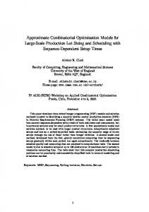
The development of the TPM model uses the following general approach: 1. Write the control rules of the model into equations that relate production quantities to queue length quantities. 2. Write equations describing work arrivals for each station. Include work arriving to the station from outside the network, and work arriving as a result of production at upstream stations. 3. Substitute the control-rule and work-arrival equations into the standard inventory balance equations to each station, yielding a single set of recursion equations relating work (or queue lengths) completed in the last period to work (or queue lengths) in the current period. 4. Iterate the recursion equations infinitely, which will yield a power series expression for the steadystate production (or queue lengths) at all stations. Take the moments of this expression to find the steady-state expectation and variance of production (or queue lengths). 5. Use the control-rule equations to calculate the moments of the queue lengths (or production quantities, if the recursion equations were written in terms of queue lengths). We will use this approach repeatedly to develop and analyze more complicated MR models. We begin with a simple extension, the application of the TPM to base stock models. For example, we use this approach to analyze models with general linear control rules, discussed in Chapter 4. Models with general control rules, along with the other models we consider in later chapters, are significantly more complicated than the TPM, but we will use the same basic approach to analyze them. Example: Base Stock Models. As an example, we use the approach to derive an extended TPM that models base stock job shops. As written, the TPM assumes that work enters from outside the shop enters at particular stations (from order requests, for instance), and that this work then pushes its way through the network. In this section we consider a modification to this “push” model, called a base stock job shop. Here, completed products are stored in a buffer. Each time an item is removed from the buffer, the buffer sends an order to make a new item. Figure 1 diagrams a single -product base stock job shop.
28
Chapter 2: Models with Linear Control Rules
Workstations
Buffer
Demand
Item demand creates work orders at workstations
Figure 1 -- A Base Stock Job Shop To apply the TPM to a basestock model, we first note that all stations except the buffer station behave exactly as in the original TPM. Thus, we consider removals from the buffer and the corresponding orders to the first stations in the work flows. We assume that the number of units demanded in a given period can be treated as a continuous random variable. As with work arrivals, the demand comes from a serially i.i.d. distribution with finite mean and variance. Thus, the demand from the buffer station at time t is written as ε it , except that ε it is now explicitly negative. The demand has an expected value, µ i < 0 , and a variance, Σ ii > 0 . We now model the order requests sent to the first stations in the work flow that produce the item. Suppose that station j is one of these first stations. As with all other work arrivals, the orders to replace items leaving the buffers in time t are written as ε jt ; to apply the TPM, we need to find the expectation and variance of ε jt . Let station j require h ji time, on average, to produce one unit in the final buffer. Then, removing ε it from the buffer creates − h jiε it of work at station j. Using this relationship, the expected quantity of the orders is µ j = − h ji µ i , and the variance of the incoming orders is Σ jj = (h ji ) Σ ii . Further, 2
since the orders equal a negative multiple of the units leaving the buffer, the correlation coefficient of ε it and ε jt equals –1. Therefore, the Σ ij and Σ ji entries in the input covariance matrix must be those entries that produce a correlation coefficient of –1; these entries are Σ ij = Σ ji = − (h ji S ii ) 2 . In a base stock model, the expected number of products entering the buffer equals the expected number of products demanded from the buffer. (Otherwise, either the buffer’s inventory or back orders would grow without bound.)
Since we model demand to be negative work arrivals, the expected
“production” at the buffer station will equal 0, making the size of the buffer (i.e. the buffer’s expected queue length) indeterminate. From the perspective of the model the analyst may set the buffer size as desired. In practice, we may wish to make the buffer as small as possible to meet certain performance guarantees against the probability of back orders. For example, if the product demand is approximately 29
Chapter 2: Models with Linear Control Rules normal, one may want to make the size of the buffer equal to twice the standard deviation of the “production” at the buffer. This size will provide an approximately 97% chance that the buffer will not run out of items in any particular period. We have now completed steps 1-2 of the General Approach, defining the production rules (same as the TPM) and characterizing the work arrival processes (modified for stock replenishments). Since we have now written the model parameters as TPM input matrices, we can apply the TPM momentcalculating formulas directly, completing steps 3-5 of the General Approach. As a numerical example, consider the four-workstation plus buffer model shown in Figure 1. The following table presents a set of inputs corresponding to this model. Workflow (Φ’) From Station 1 (Input 1) 2 (Input 2) 3 (Process 1) 4 (Process 2) 5 (Buffer) Demand (µi ) Covariance (Σ ) 1 (Input 1) 2 (Input 2) 3 (Process 1) 4 (Process 2) 5 (Buffer) Lead Time
1 (Input 1)
2 (Input 2)
To Station 3 (Process 1) 1.0 1.0
4 (Process 2)
5 (Buffer)
1.0 1.0 3.0 (60% demand)
2.0 (40% demand)
-5.0
0.8
-3.0 -2.0
1.8 0.10 0.10 -3.0 4 (αi = 0.25)
-2.0 4
1
5.00 1 (N/A)
1
The resulting moments of production and queue lengths are: Station
Expected Production
1 (Input 1) 2 (Input 2) 3 (Process 1) 4 (Process 2) 5 (Buffer)
3.0 2.0 5.0 5.0 0
Standard Deviation of Production 0.508 0.338 0.687 0.756 2.360
Expected Length 12.0 8.0 5.0 5.0 N/A
Queue
Standard Deviation of Queue Length 2.028 1.352 0.687 0.756 N/A
As discussed, a good estimate for the size of the buffer would be twice the standard deviation of “production” at the buffer, which here is 4.72 units (or 5 units if the buffer only stores discrete objects).
3. The Tactical Planning Model for Pull-Based Systems Much of the rest of this thesis may be seen as creating extensions and generalizations of the TPM. The first extension we consider is an adaptation allowing the TPM to model “pull-based” systems. The TPM by itself is a “push-based” system, in which each station processes a fixed fraction of the amount of
30
Chapter 2: Models with Linear Control Rules inventory in its input buffer. In 1987, however, Leong showed how to apply the TPM to “pull-based” systems, such as the popular Kanban systems. In these systems, each station now has an output buffer, from which downstream stations draw inventory; each buffer has a “target” inventory level. Production quantities no longer depend on work in the input buffer. Instead, each period each station produces enough to make up a fixed fraction of the shortfall between a target level, Ti , and the amount of inventory actually in the buffer. (For example, if the target level is 6 hours worth of on-hand inventory, the buffer only contains 4 hours of on-hand inventory, and the fixed fraction, α i , is 0.5, the station will produce one hour’s worth of inventory over the next period.) The development of the TPM for pull-based systems is very similar to that of the original TPM. The one key difference is that the inventory balance equations are no longer written in terms of Qt, the inventory actually at the stations. Instead, the balance equations are written in terms of Vt, the difference between the target inventory levels and the actual inventory levels. Mathematically, the new production rule is: Pit = α iVit , where
(26)
Vit = Ti − Qit .
The inventory-balance equation now represents the inventory shortfall in each time period: Vit = Vi ,t −1 − Pi ,t −1 + Ait ,
(27)
where Ait is work that leaves stage i’s output buffer at the start of time t, thus increasing the shortfall that must be filled. The equation for the arrivals appears the same as it was in the TPM: Ait =
∑ (φ
ij Pj ,t −1
)
+ ε ijt + N it .
(28)
j
However, the meaning of the terms is different. φ ij is the amount of work that one unit of production at stage j pulls from stage i. Nit is the quantity demanded externally from stage i at period t.
This new
characterization of work arrivals might allow one to model assembly stations that draw product components from upstream stations, for example. Despite the change in meaning of the variables, the recursion equations have remained the same; thus, the recursion equation Pt is exactly what it was for the TPM, Pt = (I − D + DF) Pt−1 + et . Consequently, we find the moments of the production and the shortfalls the same way, as well:
31
Chapter 2: Models with Linear Control Rules E[P]= (I − F ) −1 µ var[P ] =
∞
∑ B (DSDSD), where B = I − D + DF s
s
s= 0
(29)
E[V ] = D −1E[P] var[V ] = D −1var[P]D −1.
The relationship Vit = Ti - Qit immediately implies the moments of the actual inventory levels, Qt: we have that E[Qi ] = Ti – E[Vi ], and var[Qi ] = var[Vi ]. In practice, we will want to set the Ti ’s large enough to ensure that the inventory levels are non-negative.
4. The General LLS-MR Model In this chapter, we consider the general form of LLS-MR models, where production is a general linear function of the work-in-queue at multiple stations. The production rule is: (GLR)
Pit = ∑α ijQ jt + βi + γ it , j
(30)
where the parameters α ij are smoothing parameters, βi is a constant, and γit is a serially-iid random variable with zero mean and finite variance. Note that individual α ij ’s need not be between 0 and 1, provided that the resulting production is neither negative nor requires more inventory than that in queue (or is very unlikely to be negative or require more inventory than that in queue). Indeed, some α ij ’s could be negative; a negative α ij implies that production is slowed down as a queue level increases. Negative α ij ’s can model policies that seek to prevent upstream stations from sending excess inventory to downstream stations. For example, the pull networks discussed in section 3, which produce work to eliminate shortfalls at downstream stations, may be modeled using (GLR). Similarly, the pull network formulation discussed in section 3 models general control rules with negative α ij ’s. The formulation of a general control rule for pull networks is: Pit =
∑α V ij
jt
j
+ β i + γ it ,
where Vjt is the inventory shortfall at station j at time t. With this convention, all α ij ’s are positive. Further, Vjt does not need to be positive. A negative Vjt implies that a queue has too much inventory, so that upstream stations will reduce production.
32
The expanded Vit allows the modeling of
Chapter 2: Models with Linear Control Rules “counterbalancing” control rules; we will present an example of a model that uses counterbalancing control rules (the Denardo-Tang model) in the next section.
4.1
Motivation for the General LLS-MR Model
Control Theory. The use of general linear control rules has an important advantage: if the objective of the shop is to minimize a quadratic cost function of production and inventory levels, a linear control rule will minimize the objective. For example, consider the following dynamic minimization problem:
(V-MIN)
∞ min E d t [(Pt − E[P])′CP (Pt − E[P]) + (Qt −1 − Q*)'CQ (Q t−1 − Q*)] t= 0 s.t. Q t = Q t −1 + (F − I )Pt −1 + e t , ∀t ,
∑
(31)
where d is a discount factor, Q* is a vector of target queue levels, CP is a matrix setting the cost for production quantity fluctuations, and CQ is a matrix setting the cost for queue le vel fluctuations. The objective function seeks to minimize the variances of production and queue lengths over a discounted infinite time horizon. The recursion equations for Qt are the TPM recursion equations, with ε t being a serially-i.i.d. noise vector, as previously discussed . Consequently, problem V-MIN seeks the production quantities that will minimize the production and queue length variances within a discrete-time manufacturing model over an infinite discounted time horizon– a problem we expect might be of great interest in a variety of manufacturing applications. The solution to V-MIN will be discussed in detail in Chapter 7, which examines dynamic control of MR-models. For now, however we state that the formula for the optimal production quantities will be a linear function of the queue lengths of the form:
Pt = E[P] + K t (Q t − Q*) ,
(32)
where Kt is a matrix. Further, in steady state, Kt will converge to a constant matrix K provided that d < 1. (These results come from the application of dynamic programming theory to linear systems with quadratic cost; see, for example, Bertsekas (1995a)). Then, the optimal steady-state production quantities in the discrete-time manufacturing model will be given by a general linear control rule. Processing Time Predictability. In addition to minimizing production and queue length variances, linear control rules make waiting times predictable, as well. In the single -station example in Section 2, 96% of all the work in queue waited between 4 and 6 periods, despite fairly high fluctuations in the arrival stream to the station.
33
Chapter 2: Models with Linear Control Rules Modeling of Adaptive Control Rules. Beyond optimal policies for quadratic -cost systems, the general LLS-MR model allows the analyst to model other control rules which modify station production rates to limit production and inventory fluctuations throughout the entire shop. This modeling ability is important for just-in-time manufacturing applications, for instance. One example of adaptive control rules is the proportional restoration control rule suggested by Denardo and Tang (1997). These rules are pull models where stations’ productions are controlled by the need to restock downstream inventories. In particular, the production at each station is the amount needed to restock some fraction of the shortfall across all downstream inventories. Job shops with proportional restoration rules will be discussed in the next section.
Production Fluctuations . Allowing random fluctuations in production quantities is also an important extension. This addition allows the analyst to model situations in which production does not depend exactly on queue lengths – which will likely include many situations. Empirical Evidence for Linear Control Rules. There is empirical evidence that stations may follow linear control rules in practice. For example, Fine and Graves (1989) showed that many stations at a mainframe subcomponent manufacturing plant empirically obeyed a linear control rule.
4.2
Model Development
We develop the general linear control rule model for push networks. The equations for pull networks are similar, except that the Qt’s are replaced by Vt’s. We write the production rules simultaneously in matrix-vector form as: Pt = DQ t + ß + ? t , or Q t = D−1 (Pt − ß − ? t ) .
(33)
Here, D is a non-diagonal matrix, assumed to be non-singular. Solving the equation for Qt and substituting the results into the inventory balance equation, Qt = Qt-1 – Pt-1 + At, yields:
D− 1 (Pt − ß − ? t ) = D− 1 (Pt −1 − ß − ? t −1 ) − Pt−1 + At , where A t = F Pt −1 + et ⇒ Pt = (I − D + DF )Pt −1 + Det + ( ?t − ?t −1 ).
(34)
The constant production term, β, cancels out of (30). The term will reappear in the equations for the queue length moments, however. By iterating (30) and assuming an infinite history of the system, we find the following power series equation (similar to the results for the TPM):
34
Chapter 2: Models with Linear Control Rules ∞
Pt = ? t + ∑ B s (De t −s + (B − I)? t −s−1 ), s =0
(35)
where B = I − D + DF . Since the mean of γ t equals zero, E[P] is:
E[P] = (I − B)− 1 Dµ = (I − F )−1 µ.
(36)
The expected production in this model is exactly the same in the general linear model and in the TPM. This is not a coincidence. In the next chapter, we will show that if the production rule is any general function of the queue lengths such that the resulting network is stable, the expected production at each station will always be E[P] = ( I − F )−1 µ . The steady-state variance of P is similar to what it was for the TPM. To account for the γ t’s, we add an additional term to the infinite series: ∞
S = var( Pt ) = Γ + DΣ D'+∑ B s ( DΣ D'+(B − I)G(B − I) ')B's , s =1
(37)
where B = I − D + DΦ , and G = cov( ? t ) The moments of Pt imply the moments of the queue lengths, Qt: E[Q] = D −1 (E[P] − ß ), and
var[Q ] = D −1 (S − G)(D−1 )'
(38)
The calculation of E[Q] follows directly from the equation Q t = D −1 (Pt − ß − ? t ) . The calculation of var[Q] is a more subtle. Note that γ t appears in the recursion equation for Pt, whereas − ? t appears in the equation for Qt. Thus, the contribution of γ t is negated, so the variance of γ t must be removed from the variance of Qt. (This is not an issue with E[Q], since E[γ t] = 0.) For pull models, we find the moments of the shortfalls, E[V] and var[V] rather than E[Q] and var[Q].
We find the moments of the queue le ngths using the same formulas as the TPM for pull
networks: E[Q] = T − E[V] , where T is the vector of target inventories, and var[Q] = var[V] .
5. Example: A Stochastic Production System Using Proportional Restoration Control Rules In this section, we apply general linear control rule models to a stochastic production system using the proportional restoration rules developed by Denardo and Tang (1997). As discussed, these rules are pull 35
Chapter 2: Models with Linear Control Rules models where stations’ productions are controlled by the need to restock downstream inventories. In particular, the production at each station is the amount needed to restock some fraction of the shortfall across all downstream inventories. We first derive the MR model that uses proportional restoration rules, and then apply the model to a problem suggested by Denardo and Tang (1997).
5.1
Model Development
Mathematically, the production of station i at time t is given by:
Pit = E( Pi ) +
∑ (E (Q ) − Q )r Φ N
j
jt
j
∗ ij
+ γ it ,
(39)
j:Φ ji >0
or, in accordance with the notation of the pull models,
Pit = E ( Pi ) +
N
∑r Φ V j
∗ ij
jt
+ γ it
(40)
j :Φ ji > 0
Here, E(Qj ) is a target buffer size, or desired queue level for station j, rj is a control factor set by the user such that 0 ≤ rj ≤ 1 , and Φ ∗ij is the estimated work that must be completed at i to get one unit of work to arrive at station j. In words, this rule says that the production at station i is the expected production plus or minus a restoration quantity that partially restores the queues at downstream stations to the desired expected queue lengths.
On average, rj of the shortfall (or excess) at station j will be restored each
period. As with the TPM models discussed previously, we continue to assume that ε t represents fluctuations in work arrivals. As before, ε t is a serially-i.i.d. random variable with mean µ and covariance matrix Σ . The proportional control rule is a general linear control rule for a pull network with:
α ij = r jΦ *ij , β i = E ( Pi ), and γ it is a serially - iid random variable with zero mean.
(41)
To use the model equation derived in the previous section, we simply need to find the E(Pi )’s and Φ ij *’s. As discussed in the previous section, regardless of the α ij ’s, E ( P) = (I − F )−1 µ . Using the derivation of pull models discussed in Section 3, Φ ∗ij equals the expected amount of work one unit of demand at station j induces at station i. Thus, each Φ ∗ij element is the (ij) element of the matrix F * = (I − F )−1 .
36
Chapter 2: Models with Linear Control Rules We apply the equations in Section 4 directly, yielding E(P), var(P), E(V), var(V), E(Q), and var(Q). E(V) merits a special comment; using the formula in Section 4, we see that
E[V ] = D −1 (E[P] − ß) = D −1 (E[P] − E[P] ) = 0 ,
(42)
implying that the expected queue lengths will be whatever the target buffer sizes are. Mathematically, we have freedom to choose any target buffer sizes. In practice, we want to choose target buffer sizes large enough that the probability of stockouts are small. If the production fluctuations are approximately normally distributed, a good choice is to make the buffer sizes twice the standard deviation of the queue lengths (this is the approach recommended by Denardo and Tang (1997)).
This rule gives rise to
nonlinear programs to find the rj ’s minimizing the required buffer sizes; these nonlinear programs will be discussed in some detail in Chapter 6, on the optimization of MR Models. We conclude the development by noting that Denardo and Tang’s model is not a MR model. Denardo and Tang modeled production systems using an underlying Markov chain, such that production fluctuations are due to work discarded in accordance with a binomial distribution. They also assumed that the shop contains no cycles in the work flows. The MR-models behave differently. They do include a Markov assumption that work requirements at a station do not depend on how a particular workflow got to that station. However, instead of Binomial distributions, the fluctuations in production and work transfers may be modeled by any distributions independent from the production and queue length quantities. The latter assumption prevents MR models from directly copying Denardo and Tang’s models, since the latter’s production variances are directly proportional to the amount of work produced. Further, MR-models do allow cycles in work flows; transitions showing work returning to upstream station are treated like any other transitions. The latter ability models job shops that subject items failing quality tests to rework, for example.
5.2
An Example Production System
Denardo and Tang (1997) present a six-station assembly line controlled using proportional restoration rules. Finish products are removed from the buffer at station 1, while station 6 receives inventories from an infinite source. The assembly line is shown in Figure 2. Buffer
Station
Demand 1
2
3
4
Figure 2 – A Six-Station Assembly Line
37
5
6
Source
Chapter 2: Models with Linear Control Rules External demand at station 1 is Poisson with a mean and variance of 20 units. At each station, the failure rate is 15%, so one unit of demand at station i induces an average of 1/.85 units of demand at station i + 1. As discussed, we cannot model Binomial-distribution failures directly with MR-models, so we approximate the variance caused by failures at each station to be Σ ii = E ( Pi )( 0.15)(0.85) , using the fact that the true variance of Binomial distribution failures would be Σ ii = Pi (0.15)( 0.85) . (This particular approximation underestimates the variances somewhat.) Finally, Denardo and Tang suggest the control parameters r1 = 0.25, r2 = 0.35, r3 = 0.43, r4 = 0.51, r5 = 0.60, and r6 = 0.68. Together, these inputs yield the following model parameters: Workflow, Φ ’ From Station 1 2 3 4 5 6 Demand, µi Expected production, E(Pi) Input variance, Σ ii ri
To Station 1
2 1.176
3
4
5
6
1.176 1.176 1.176 1.176 23.53 20/0.85 = 23.53 23.53*0.15*0.85 + 20 = 23.00 0.25
0 23.53/0.85 = 27.68 27.68*0.15* 0.85 = 3.53 0.35
0 32.57
0 38.31
0 45.07
0 53.03
4.15
4.88
5.75
6.76
0.43
0.51
0.60
0.68
Running the model yields the following results. Note that the recommended buffer size is twice the standard deviation of the queue length: Station
Expected Production
1 2 3 4 5 6
23.53 27.68 32.57 38.31 45.07 53.03
Standard Deviation of Production 2.51 2.87 3.30 3.79 4.36 5.03
Standard Deviation of Queue Lengths 7.25 3.65 3.66 3.74 3.86 4.05
Recommended Buffer Size 14.50 7.30 7.32 7.48 7.72 8.10
6. Example: A Communications Problem 6.1
Introduction Linear-MR models provide a great deal of flexibility to model (and optimize) a wide variety of
situations which can be represented by a “processing network.” Here, we consider a communications application similar to capacity-allocation problems faced by the US Department of Defense.
38
Chapter 2: Models with Linear Control Rules In this example, a set of antennas broadcast signals at probabilistic intervals; broadcasts may be correlated (positively or negatively) with each other. Each broadcast signal uses a random amount of bandwidth with a finite mean and standard deviation. These signals are received by a set of remote receivers; each receiver transmits the signals it receives to a communications satellite, which transmits collections of signals to a central base. Analysts at the central base then send control signals back to the remote receiver stations requesting additional information about particular signals, which the receiver stations provide through the same connections as the original signal. It is assumed that a receiver or a satellite cannot store signals; signals must be transmitted immediately or dropped. The objective is to determine how much bandwidth must be installed at each receiver and satellite to meet certain levels of service (i.e. avoid dropping too many signals.) Figure 3 graphically shows the situation. Broadcast Antennas
Receiver Stations
Communications Satellites
Central Base (Analysis) Data signal Control signal
Figure 3 -- A Communications Example from the Department of Defense
6.2
Model Development At first glance, this scenario appears not to be relevant to MR models; no work is queued
anywhere in the model, and the Markovian assumption is not satisfied directly (different signals require separate handling by the same receivers, satellites, and analysts). However, this situation is amenable to MR modeling with a few minor adjustments. First, “no work queued anywhere in the system” is equivalent to requiring the lead times at all stations to be one. This forces the stations to process all work within a single period. Assuming the “period” for this communications period is quite short (a second or less), the resulting MR model should realistically represent near-instantaneous communications. Second, the signal bandwidth at any time is
39
Chapter 2: Models with Linear Control Rules the same across all stations handling that signal, since the bandwidth depends on the signal itself, not interactions between stations handling the signal. Thus, in the MR model, we have one station that “transmits” the signal; this station sends work flows directly to all the stations that receive the signal. For example, a signal’s “antenna” station directly sends work to a receiver station, a satellite station, and a base station. The receiver station, satellite station, and base station do not send work to each other. To address distinct signal handling, we add stations to the model as follows: there is one dummy station representing every particular signal handled by a particular communications station (receiver, satellite, or analysis base). We then apply the steady-state moment equations to the resulting “extended” model. Using the linearity of expectation, we know that the expected throughput at a communications station is the sum of all the dummy stations associated with the station. The variance of the throughput is the sum of the variances of the dummy stations, plus all the covariance terms between those stations. The covariance terms are especially important in this case; in addition to multiple signals being correlated with each other, all the stations that handle a single signal are perfectly correlated with each other as they will see the exact same bandwidth at any given time. Knowing the expectation and variance of the throughput implies how much capacity will be needed to meet desired levels of service; the capacity that needs to be assigned to each communications station is given by:
Ci = E[ Pi ] + k i var( Pi ) ,
(43)
where Ci is the required capacity, and k i is a safety factor used to translate variance of production information into level of servic e requirements. A factor of 2 is often used in practice, since, if the production levels were normally distributed, the resulting capacity would be able to handle the required load about 97% of the time. In our scenario, however, “production levels” (i.e. data signals) will not be normally distributed given that they are convolutions of a distribution determining whether a source is broadcasting and a distribution determining how much data is generated assuming the source is broadcasting. Thus, simply applying a safety factor of 2 will be inappropriate. Nonetheless, there are more appropriate ways to calculate the safety factors. We will discuss an analytic approach to estimating the needed safety factor at the end of this section. Alternately, analysts may perform simple Monte-Carlo simulations to translate the expectation and variance results to capacity levels required to meet service requirements. These simulations would be simple single -distribution runs that could be completed in a few tenths of a second; discrete event simulations are not required. We now present a small example of the communications problem. We have six broadcast antennas, three receivers, and two communications satellites. The six antennas can be divided into three groups, with 1, 2, and 3 antennas per group. If two antennas are in the same group, their broadcasts are 40
Chapter 2: Models with Linear Control Rules positively correlated; if two antennas are in different groups, their broadcasts are independent. Figure 3 (presented previously) shows how the three groups of antennas, the receiver stations, and the communications satellites communicate with each other. To model this scenario in terms of a linear MR model, we create one work station for every particular signal handled by a communications device. Here, each signal travels through a receiver, a satellite and a base; the signal then creates a corresponding control stream that travels from the base, back through the satellite to the receiver. Thus, there are six stations per signal: one representing the broadcast antenna, one representing the base, and four representing the data and control streams to and from the receiver and satellite. Since there are six signals, the model has a total of 36 stations. Figure 4 shows the signal flows between the stations that will be used in the MR model.
Data Flow (d) Broadcast Antennas Group A
Receivers
Control Flow (f)
Comm Satellites
Central Base (Analysis)
Comm Satellites
Receivers
a1 a2
r1
s1
b
s1
r1
a3 Group B
Group C
a4
r2
s2
b
s2
r2
a5
r3
s2
b
s2
r3
a6 Figure 4 – Signal Flows in the Physical Communications Network
In the figure, the arcs represent data flows between stations. Note that not all the arcs between the control-flow receiver stations and the data-flow receiver stations are shown. The boxes group the stations that correspond to a processing step for a correlated group of signals on a single piece of equipment. For example, there is a box corresponding to receiver r1 processing all signals within signal group 1. Although Figure 4 shows all the stations in the MR model, and the physical signal flows between these stations, the figure does not show the actual layout of the model. As previously discussed, all the stations handling a given signal will see the same bandwidth at any time (data stations will see the whole signal, and control stations will see a fraction of the signal). It is not the case that the stations transmit
41
Chapter 2: Models with Linear Control Rules signal chunks across multiple time periods. This situation is modeled accurately by having each signal’s antenna station send work to the stations that receive the signal simultaneously. Figure 5 shows the antenna stations broadcasting to the receiver, satellite, and base stations simultaneously, and thus shows the true layout of the MR model.
Broadcast Antennas
Receivers (Data)
Comm Satellites (Data)
Receivers (Control)
Comm Satellites (Control)
Central Base (Analysis)
a1 a2 Group A
Group B
Group C
a3
r1
s1
a4 r2 a5 a6
r3
s2
b
Figure 5 -- Model Representation of the Network Example Figure 5 also shows the stations that comprise the signal handling required by each communications device. Recall that we are most interested in the aggregate capacity required for each communications device, which involves combining the results for all the stations corresponding to a piece of communications equipment. For example, the aggregate capacity on communications satellite s2 is a function of the six stations in the box labeled “s2”. We are also interested in the aggregate capacity throughout the system required for a particular signal. This estimate involves combining the results for all the stations corresponding to that signal. For example, the aggregate capacity required by group 1’s third signal is a function of all the stations connected to station a3. As noted, the aggregate capacity recommended for a device is a function of the expectation and variance of the total throughput through that device. The total expected throughput equals the sum of the
42
Chapter 2: Models with Linear Control Rules expected throughputs at all stations corresponding to that device. The total throughput variance equals the sum of all the variance and covariance terms between the stations corresponding to the device. The time required to estimate the throughput moments is proportional to the cube of the number of stations. While 36 stations should not be a problem, stations with hundreds or thousands of signals could cause serious computational difficulties. Fortunately, in this problem we can decompose our single model representation into multiple representations. In our models, stations that correspond to separate signals do not send information to each other. The only way these stations interact with each other at all is if their corresponding signals are in the same group (i.e. correlated with each other). If not, the stations do not interact with each other, so any aggregate results will not reflect any interactions between the stations. Thus, we can decompose the single model into a completely separate model for the stations corresponding to signals in each group. In our example, we therefore have three independent models, shown in Figure 3 by the lines separating the “Group A”, “Group B”, and “Group C” stations. If a communications device is represented in multiple models (for example, the satellite s2), its aggregate expected throughput is the sum of the corresponding expected throughputs for each model, and the aggregate throughput variance is the sum of the corresponding throughput variances for each model. (The latter statement holds since all covariance terms between stations in separate models are zero.)
6.3
Converting System Data to Model Inputs We have the following numerical data for each signal:
Signal Signal Group Broadcast Probability Broadcast Correlation Coefficient for Group Mean Signal Bandwidth (Mbits/sec) Standard Deviation of Signal Bandwidth (Base)
1 A 0.2 0.3 2 0.2
Mean Bandwidth of Corresponding Control Stream 0.2 as a fraction of signal bandwidth Standard Deviation of Control Bandwidth 0.1 Standard Deviation of Signal Bandwidth that results 0.2 from control stream instructions
2 A 0.3 0.3 3 0.05
3 A 0.1 0.3 4 1.5
4 B 0.05 0.5 10 5
5 B 0.15 0.5 1 0.8
6 C 0.2 NA 5 2
0.3
0.4
0.2
0.2
1
0.1 0.2
0.1 0.5
0.1 1
0.1 0
0.4 0.5
We now use this numerical data to define the matrices used in the MR equations. In defining the entries for the matrices, we use the following subscripts: •
a: broadcast antenna station
•
r: receiver station
•
s: satellite station
•
b: central base
43
Chapter 2: Models with Linear Control Rules •
d: station that is part of a signal data flow to the base
•
f: station that is part of a control flow from the base
•
i,j: indices of a particular signal
•
k,l: indices of a particular communications device
Entries for broadcast antenna stations . These are the only stations that receive arrivals from outside the network of stations, representing the generated signals. Three factors enter into the matrix entries. First, each station has a probability that it will broadcast at any particular time.
Second, these
broadcasting periods are positively correlated with each other. Third, when broadcasting, each station generates a signal according to a random distribution with the mean and standard deviation given above. Then, the overall mean signal generated by antenna station ai is:
µ ai = pai mai ,
(44)
and the input variance of the signal generated by antenna station ai is: Σ ai,ai = p ai sai2 + p ai (1 − p ) ai (m ai ) 2 ,
(45)
where p ai is the probability that station ai is broadcasting, mai is the mean bandwidth when the station is broadcasting, and sai2 is the variance of the bandwidth when the station is broadcasting. (These formulas both result from the moment formulas for a random sum of random variables.) The covariance between each pair of broadcast stations in the same group is:
Σ ai, aj = ρai, aj m ai pai (1 − pai )mbi paj (1 − paj ) ,
(46)
where ρ ai,aj is the correlation coefficient between the broadcasting of stations i and j. As discussed, the covariance between stations not in the same group is 0, which for separate models representing each group of signals. Note also that the covariance does not depend on the variance of the bandwidth when the stations are actually broadcasting, because signal bandwidths are assumed to be independent. We conclude by noting that the broadcast antenna stations do not receive any flow from other stations. Thus, all workflow matrix (Φ ) entries representing expected work arriving from other station to antenna stations equal 0. Entries for receiver stations . There are two sets of receiver stations; the first set represents signal data (marked by subscript d), and the second set represents control flows (marked by subscript f).
44
Chapter 2: Models with Linear Control Rules We consider the signal-processing stations first. The base signal that enters the receiver station is the same signal emitted from the broadcast antenna. Thus, the workflow matrix entry representing flow between antenna and receiver stations equals 1, or:
Φ rdi, ai = 1, for all signals i. The control flow for each signal affects the amount of the base signal that the signal-processing stations have to transmit. This effect is modeled through a random variable with zero mean and a finite variance. It is the only effect that adds to the variance of the throughput at this station. Thus, the input variance for signal-processing stations is: 2 Σrdi,rdi = σ rsi , rfi ,
where the second term is the variance that control-flow station rfi induces at station rsi. We next consider the control-processing stations. They receive the control flow transmitted to them by their communications satellite. As previously discussed, this transmission is modeled by a direct flow from the signal’s antenna station to the receiver station. Thus, the workflow matrix entries are: Φ rfi, ai = φ fi , for all signals i,
where φ fi is the expected control bandwidth as a percentage of the signal bandwidth. The input variance entries are: Σ rfi, rfi = σ 2fi , for all signals i,
where σ 2fi is the variance of the control bandwidth.
Entries for satellite stations . Again, there are signal data and control flow satellite stations. Signal data stations receive the signals passed to them their receivers, which is just the base signal data. Then the workflow matrix entries are: Φ sdi,ai = 1 , for all signals i.
The input variance entries are the same as for the data receiver stations. The signal fluctuations entering the receiver station are duplicated in the satellite stations, since the communications satellite does not alter the signal data it receives. The only signal fluctuations result from the influence of the signal control flows, as described in the discussion of data receiver stations. Thus, the input variance entries are: 2 Σ sdi, sdi = σ rsi ,rfi ,
the same as the data receiver stations. Control-flow satellite stations are the first stations to receive control signals (broadcasted from the base), but this fact is of little modeling significance; like all other stations, they receive work directly
45
Chapter 2: Models with Linear Control Rules from the their signal’s antenna station. Thus, the workflow matrix entry representing the control signal’s flow equals: Φ sfi,bi = φ fi , for all signals i,
where the second term is the expected control bandwidth as a percentage of the signal bandwidth. The input variance entries are: Σ sfi, rfi = σ 2fi , for all signals i,
where the second term equals the variance of the control bandwidth Entries for base stations . There is only a single set of base stations, which both receive signals from the satellites and transmit control flows to the communications satellites.
In the model, only the base
stations’ receipt of the data signal appears, since all stations receive work from their signal’s antenna station. Base stations receive the same bandwidth as the other data stations. Thus, the workflow matrix entries are: Φ bi,ai = 1 , for all signals i,
and the input variance entries are: .
2 Σ bi,bi = σ rsi ,rfi ,
where the second term shows the influence of the control flow on the amount of the base signal transmitted.
6.4
Calculating the Results
We have developed MATLAB scripts that convert the signal data into model inputs, generate the resulting three MR models (one model for each group), calculate the throughput moments for each station, and aggregate the results for each communications device in the system. The results are shown below. The following table displays the expected throughput in Mbits/sec (first number) and standard deviation of the throughput (second number) for each of the 36 stations in the model. Signal 1 2 3 4 5 6
Antennas 0.4 0.8 0.9 1.38 0.4 1.29 0.5 2.45 0.15 0.53 1 2.19
Signal Data Receivers Satellites 0.4 0.83 0.4 0.83 0.9 1.39 0.9 1.39 0.4 1.38 0.4 1.38 0.5 2.65 0.5 2.65 0.15 0.53 0.15 0.53 1 2.25 1 2.25
Base 0.4 0.83 0.9 1.39 0.4 1.38 0.5 2.65 0.15 0.53 1 2.25
Signal Control Satellites Receivers 0.08 0.19 0.08 0.19 0.27 0.43 0.27 0.43 0.16 0.84 0.16 0.84 0.1 0.54 0.1 0.54 0.06 0.23 0.06 0.23 1 2.25 1 2.25
We then find the expectation and standard deviation for the throughput for each communications device. Recall that the 36 stations each correspond to the data or control processing of one signal on a particular 46
Chapter 2: Models with Linear Control Rules device; the stations corresponding to each device were labeled in Figure 2. The expected throughput on a device equals the sum of the expected throughput of each of the device’s stations. The variance of a device’s throughput equals the sum of all of the variance and covariance terms of each of the device’s stations. The following table displays the expectation and standard deviation of the throughput for each of the communications devices. The table also displays the signal flows processed by each device. Communications Device Antenna 1 (a1) Antenna 2 (a2) Antenna 3 (a3) Antenna 4 (a4) Antenna 5 (a5) Antenna 6 (a6) Receiver 1 (r1) Receiver 2 (r2) Receiver 3 (r3) Satellite 1 (s1) Satellite 2 (s2) Base (b)
6.5
Signals Processed 1, data 2, data 3, data 4, data 5, data 6, data 1, 2, 3, data and control 4, data and control 5,6, data and control 1, 2, 3, data and control 4, 5, 6, data and control All, data
Expected Throughput
Standard Deviation 0.4 0.9 0.4 0.5 0.15 1 2.21 0.6 2.21 2.21 2.81 3.35
0.8 1.38 1.29 2.45 0.53 2.19 3.4 3.11 4.73 3.4 5.66 4.45
Interpreting the Results
6.5.1 Single Station Results Recall that the recommended capacity for each station (and communications device) is a function of the expectation and standard deviation of the throughput at that station, as follows:
Ci = E (Ti ) + ki ⋅ σ Ti , where Ci is the recommended capacity for station i, E(Ti ) is the expected throughput, σTi is the standard deviation of the throughput, and k i is the “safety” factor that converts the standard deviation of the throughput to a performance guarantee. This equation is well-defined except for k i . As discussed, a k i of 2 is not appropriate in this scenario. The throughput distributions are not normally distributed – they are the convolution of a Bernoulli trial and a general distribution. Usually, the throughput is 0, corresponding to the antenna not broadcasting a signal. Other times, with probability p i , the throughput’s value will come from the distribution for a signal’s bandwidth given that the signal is being broadcast. Thus, setting the safety factor to 2 does not translate to a performance guarantee. However, we can use the fact that the distribution at each station is a convolution of a Bernoulli trial and another distribution to generate more appropriate k-factors for individual stations.
The
Department of Defense is interested in performance guarantees conditional on a signal actually being transmitted. For example, the Department might wish to guarantee that a signal, when transmitted, has a
47
Chapter 2: Models with Linear Control Rules 97% chance of being processed at any given moment. Assuming the distribution for a signal’s bandwidth is approximately normal, the capacity needed to process the signal is: Ci = E (Bi ) + 2 ⋅ σ Bi ,
where E(Bi ) is the expected bandwidth of the signal, and σBi is the standard deviation of the bandwidth used by the signal, when transmitted. We would like the capacity recommendations that result from the throughput moments and the above equation to be the same. Thus, we can equate the two formulas for capacity and solve for k i :
E (Ti ) + ki ⋅ σ Ti = E ( Bi ) + 2 ⋅ σ Bi ⇒ ki =
E ( Bi ) − E (Ti ) + 2 ⋅ σ Bi . σ Ti
(47)
The terms E(Ti ) and σTi are given by the MR model, while E(Bi ) and σBi are not known directly. However, we now use the fact that the throughput distribution at each station is a convolution of a Bernoulli trial (whose parameter, p i , is known ) and the distribution for the signal’s bandwidth given the signal is being transmitted. The moments of the latter distribution are simply E(Bi ) and σBi . We then solve the expressions for the throughput moments for E(Bi ) and σBi . We first find E(Bi ):
E (Ti ) = pi E( Bi ) ⇒ E ( Bi ) = E (Ti ) / pi .
(48)
Similarly, we find σBi :
σ Ti2 = piσ Bi2 + pi (1 − pi )( E ( Bi ) )2
(
)
⇒ σ Bi2 = σ Ti2 / pi − (1 − pi )( E ( Bi ) )2 ⇒ σ Bi =
(σ
2 Ti
(49)
)
/ pi − (1 − pi )( E ( Bi ) )2 .
Substituting, we find the desired expression for k i :
ki =
(1 / pi − 1)E(Ti ) + 2 ⋅
(σ
2 Ti
)
/ pi − (1 − pi )(E (Ti ) / pi )
σ Ti
2
.
(50)
The following table shows the resulting safety factor and recommended capacity for each of the 36 stations in the example model. Note that most of the safety factors are significantly greater than 2.
48
Chapter 2: Models with Linear Control Rules
Signal 1 2 3 4 5 6
Antennas ki Ci 2.48 2.40 1.60 3.10 5.11 7.00 7.96 20.00 5.41 3.00 3.65 9.00
Signal Data Receivers Satellites ki Ci ki Ci 3.11 2.98 3.11 2.98 2.04 3.74 2.04 3.74 5.75 8.36 5.75 8.36 8.66 23.42 8.66 23.42 5.41 3.00 5.41 3.00 3.82 9.58 3.82 9.58
Base ki 3.11 2.04 5.75 8.66 5.41 3.82
Ci 2.98 3.74 8.36 23.42 3.00 9.58
Signal Control Satellites Receivers ki Ci ki Ci 4.09 0.85 4.09 0.85 2.35 1.27 2.35 1.27 5.32 2.96 5.32 2.96 8.18 4.19 8.18 4.19 5.54 1.35 5.54 1.35 3.90 9.90 3.90 9.90
6.5.2 Commmunications Device Results (Multiple-Station Results) The above results apply to single stations. However, planners are most interested in determining capacity for communications devices, which comprise multiple stations.
Again, the recommended
capacity is a function of the expectation and standard deviation of the device’s throughput, as follows:
Cd = E (Td ) + k d ⋅ σ Td ,
(51)
where d is the index of the communications device. Let D be the set of model stations that comprise device d. Due to the linearity of expectation, and the bilinearity property of covariance, we find:
E (Td ) = ∑ E (Ti ), i∈D
σ Td =
∑ ∑ cov(T , T ). i ∈D j ∈D
i
(52)
j
The model computes the expectation terms for every station, the variance of every station, and the covariance of every pair of stations.
Thus, E(Td ) and σTd are readily calculated. This leaves the
calculation of the safety factor. As before, simply setting k d to be 2 will be unsatisfactory, as the throughput distribution is not approximately normally distributed. Unfortunately, determining k will be much more complicated for communications devices than for individual stations, as the device represents the throughput of multiple signals rather than a single signal. Each signal has its own underlying Bernoulli process and performance requirements. The complexity of the situation is compounded by the fact that the joint distribution of signal broadcasts can be quite complicated (since we allow signal broadcasts to be correlated). We consider two strategies for estimating device capacities. Exact Strategy. The first strategy assumes perfect knowledge of the joint distribution of the signal broadcasts. It has the following steps:
49
Chapter 2: Models with Linear Control Rules 1. Calculate the Ci ’s, the capacities required for each individual signal at a particular device when that signal is broadcasting. We create a separate MR model corresponding to each signal that includes only the stations corresponding to that signal. The model inputs assume that the signal is always broadcasting (p i = 1).
The result will be the expectation and variance of the signal’s throughput
when broadcasting. We thus find each Ci to be Ci = E (Ti ) + 2 ⋅ σ Ti . 2. Use the Ci ’s and the joint distribution of the signal broadcasts to find the Cd ’s, the capacities required at each communications device. We consider all combinations of signal broadcasts that might flow through a particular device. For each combination, we multiply the probability of the combination times the capacity required to process the combination (sum of the Ci ’s for the signals being broadcast). This gives us the combination’s mass (the fraction of all signals flowing through the device that will fall into that particular configuration). We then order all the combinations by the capacity required for each combination. Then, using the mass information, we choose a Cd such that the total fraction of all the signals successfully processed by the device meets a performance requirement for that device.
We do this by making Cd large enough to process enough signal
combinations to meet the performance requirement. If very precise capacity estimates are needed, this method may be required. However, the method is complicated, and may not be tractable if many signals flow through a particular device. Approximate Strategy. This method uses the expectation and standard deviation of the throughput of the device directly to recommend a capacity for the device. As previously stated, however, the difficulty with this method is calculating the device’s safety factor, k d . Here, we approximate k d to be the weighted sum of the safety factors of the stations comprising the device. The weights are the normalized expected throughputs at each of the stations. Specifically, we approximate k d to be: kd =
∑ ∑
i∈ D
k i E[Ti ]
E[Ti ] i∈D
.
(53)
The justification for this safety factor: at any time, the bandwidth demand on the device is some combination of demands required by separate signals. Each signal’s demand requires a certain safety factor, k i . The probability that a certain amount of demand is due to a partic ular signal is the expected bandwidth of that signal divided by the total expected bandwidth.
Thus, the expected safety factor
required for any particular unit of demand is given by the above equation for k d . The following table shows the safety factor, k d , for each communications device in the example model. 50
Chapter 2: Models with Linear Control Rules Communications Device Antenna 1 (a1) Antenna 2 (a2) Antenna 3 (a3) Antenna 4 (a4) Antenna 5 (a5) Antenna 6 (a6) Receiver 1 (r1) Receiver 2 (r2) Receiver 3 (r3) Satellite 1 (s1) Satellite 2 (s2) Base (b)
Signals Processed 1, data 2, data 3, data 4, data 5, data 6, data 1, 2, 3, data and control 4, data and control 5,6, data and control 1, 2, 3, data and control 4, 5, 6, data and control All, data
Weighted k-factor
Recommended 2.48 1.60 5.11 7.96 5.41 3.65 3.26 8.58 4.01 3.26 4.99 4.28
2.40 3.10 7.00 20.00 3.00 9.00 13.27 27.26 21.20 13.27 31.05 22.40 To process signal 4: 23.42
As with any approximation based on expected values, care must be taken that the resulting recommended capacities actually meet system requirements. For example, consider the recommended capacity for the Base; it is less than the capacity required to process signal 4 by itself.
This
recommendation is not surprising, since signal 4 broadcasts infrequently in comparison to the other signals. If processing signal 4 is a requirement, however, the recommended capacity at the base station must be at least that required to process signal 4.
51
Chapter 3: Models with General Control Rules (Class GLS-MR)
1
Introduction ..............................................................................................................................53
2
The Delta Method for Production and Queue Length Moments ....................................................56 2.1 Method Development.............................................................................................................56 2.2 Recursion Equations for the Queue Lengths ............................................................................57 2.3 Recursion Equations for the Production Quantities...................................................................58 2.4 Using the Recursion Equations ...............................................................................................59
3
Steady-State Analysis for Models with Single -Queue Control Rules .............................................60 3.1 Equations for the Steady-State Moments.................................................................................60 3.2 Estimating the Steady-State Moments Using Queue Lengths ....................................................62 3.3 Estimating the Steady-State Moments Using Production Quantities ..........................................66
4
Empirical Behavior of Models with Single -Queue Control Rules..................................................71 4.1 A Single Station ....................................................................................................................71 4.2 A Six-Station Assembly Line .................................................................................................76 4.3 A Job Shop that Manufactures Mainframe Subcomponents ......................................................81
5
Steady-State Analysis for Models with Multi-Queue Control Rules ..............................................85 5.1 The Delta Method for Models with Multi-Queue Control Rules................................................85 5.2 The Multi-Queue Form of the MomentsQ Algorithm ...............................................................86 5.3 The Multi-Queue Form of the MomentsP Algorithm ................................................................88
6
An Asymptotic Lower Bound on Expected Queue Lengths ..........................................................91
52
Chapter 3: Models with General Control Rules
1. Introduction In Chapter 2, we considered LLS-MR models, which used linear control rules. These control rules were either single -queue rules (form Pit = α i Qit , where α i is a constant) or multi-queue rules (form Pit =
∑α j
ij Q jt
, where the α ij ’s are constants). In this chapter, we consider GLS-MR models. We recall
the taxonomy of MR models in Chapter 1 to identify the properties of these models: •
General control rules. Here, the control rules are general functions of the queue lengths. We will consider single -queue control rules of the form Pit = pi (Qit ) , and multi-queue control rules of the form Pit = pi (Q t ) .
•
Linear inter-station work transfers. Work arrivals from upstream stations are linear functions of the production at upstream stations plus a random noise term.
•
Stationary and independent exogenous arrivals. Work arrivals from outside the network come from stationary and independent distributions. Combined with linear work arrivals from upstream stations, we see that GLS-MR models use the arrival process discussed in chapter 2. Work arrivals are defined by A t = F Pt −1 + e t , where Φ is a constant matrix and ε t is a random noise vector. The defining feature of GLS-MR models is the fact that the control rules are general functions of the
queue lengths. Unlike linear control rules, we will not be able to find the first two moments of the production quantities and queue lengths exactly; instead, we will develop approximations of them using Taylor-series expansions. Throughout this chapter, we make the following assumptions about the control rules and other model dynamics: •
The production functions, p i (Q t ) , are continuous, twice differentiable, and monotonic over the ranges of production and queue length quantities seen by the stations in the job shop. Mathematically, these conditions hold for P min ≤ Pt ≤ Pmax and Q min ≤ Q t ≤ Q max , where Pmin and P max are vectors denoting the minimum and maximum production quantities, and Qmin and Qmax are vectors denoting minimum and maximum queue lengths.
•
The production functions have inverse functions, q i (Pt ) , that are continuous and twice differentiable over the ranges of possible production and queue length quantities. (Note that the conditions on the production functions imply the existence of the inverse production functions.) We do not require that these assumptions be met outside the ranges of possible production and queue
lengths. Thus, we can analyze control rules that violate the assumptions outside the ranges. For example,
53
Chapter 3: Models with General Control Rules we will consider control rules that become infinitely negative as Qit approaches some negative value; this is of no concern since Qit is assumed to be non-negative. Exploring models with general control rules has practical value. Below, we present some applications of models for networks using general control rules. Manufacturing. A conventional approach to job-shop capacity planning is to assume that the amount of work a station produces per period is constrained by a fixed capacity limit. This production function (called the bounded control rule) has the following form: Q , Q < M i , p i (Qit ) = it it M i , Qit ≥ M i ,
(1)
where M i is the maximum production level of station i. The capacity level has no impact on the production quantities, unless the maximum production level is reached.
Examples of this approach
include Hax (1978), Lin (1986), Baker (1993) and Bitran and Tirupati (1993). In practice, the bounded control rule often does not hold exactly. Instead, machines often show saturation or congestion effects. With these effects, machines increase their service rate somewhat to account for increased work-in-queue; for example, operators will try to push more work through a machine in a given period. However, the rate of production increases diminishes with increased work-inqueue, due to machine clogging, increased probability of quality problems, and so on. Karmarkar (1989, 1993) discussed production functions called clearing functions that account for saturation and congestion. The basic form of a clearing function is: p i (Qi ) =
M iQi β i + Qi
(2)
Here, M i is an upper bound on the service rate, and βi controls the rate at which the production approaches the upper bound. The parameter M i is the maximum production, asymptotically approached as Qi approaches infinity. The parameter βi determines the rate at which the production approaches M i . Clearing functions are continuous and twice-differentiable, making them amenable to the modeling approach we develop in this chapter. Karmarkar uses queuing theory to justify clearing functions. Consider an M/M/1 queue. Let λi be the arrival rate at station i, and let µi be the service rate. The average waiting time in an M/M/1 queue, Wi , is given by: Wi =
1/ µi , 1 − (λi / µ i )
54
(3)
Chapter 3: Models with General Control Rules Using Little’s Law, we have that Wi = Qi / λi , where Qi is the expected queue length. Substituting for Wi in (3), and solving the resulting equation for λi yields: λi =
µ iQi . 1 + Qi
(4)
More generally, for any queuing model in which the waiting time is proportional to 1 (1 − λi / µ i ) , (such as an M/G/1 queue, for example), we find that the expected arrival rate will be proportional to µi Qi (1 + Qi ) . If the queue is stable, the expected arrival rate equals the expected rate of production.
Thus, we have that the expected rate of production is proportional to M iQi (1 + Qi ) as well. Now consider a discretized version of (4). Rather than have an expected production rate (which equals the expected arrival rate), we have an expected quantity produced each time period, and an expected queue length at the start of each time period. The resulting discretized version of (4) is: E (Pi ) =
M i E (Qi ) 1 + E (Qi )
(5)
We now use (5) to suggest a control rule. We change (5) from a relationship between production and queue length moments to a relationship between the actual production and queue length quantities. The resulting control rule is: Pit =
M iQit , 1 + Qit
(6)
which has the form of a clearing function. Indeed, clearing functions are generalizations of (6), with 1 replaced by βi . Thus, queuing models, commonly used to model manufacturing networks (reviewed, for instance, by Buzacott and Yao (1986) and Suri and Sanders (1993)) suggest the use of clearing functions in discrete-period networks. Staffing in Manufacturing. Graves (1988) considers the staffing levels in a repair depot, and suggests the following piecewise linear production function: Pit = min[ Qit , K + Qit / β ] ,
(7)
where K and β are constants. At low work-in-queue levels, employees simply complete the work in the queue within a period. At higher work-in-queue levels, employees complete work according to a linear control rule. The rule at higher levels might correspond to overtime situations, for example, in which employees can only complete a portion of the additional work. 55
Chapter 3: Models with General Control Rules This piecewise linear production function cannot be evaluated directly; as a result, Graves suggests using the approximation Pit = K + Qit / β , assuming that the work-in-queue will almost always be greater than the quantity dictating that Pit = K + Qit / β .
(For reference, this quantity is
Qit = K − K / β .) This assumption will not be valid, however, for shops that regularly oscillate between
comparatively low and high demands. In such an environment, a concave production function, such as a clearing function, may be a better approximation than a linear control rule. Indeed, an analysis of the work at an actual shop may show that production quantities are better explained by a concave production function than a piecewise linear function, especially if productivity returns diminish with increasing overtime (see next example). Staffing in General. Duncan and Nevison (1996) present empirical research that compares real productivity against hours worked. They found that the resulting curve was a concave function; for example, working 60 hours yielded, on average only 50 hours of real work, and working 70 hours yielded little more. (This result applies to a single week of overtime; after 10 weeks, working 70 hours yielded only 30 hours of real work.) Section 2 presents the basic methodology used to approximate the production and queue length moments. Section 3 develops algorithms that approximate the steady-state production and queue length moments for single -queue control rules. Section 4 analyzes the empirical behavior of the approximation algorithms on a single station, a six-station assembly line, and a thirteen-station job shop that manufactures mainframe subcomponents, originally considered by Fine and Graves (1989). Section 5 extends the algorithms to multi-queue control rules. Finally, Section 6 derives a strict lower bound on expected queue lengths for concave production functions.
2. The Delta Method for Production and Queue Length Moments We assume that the control rules, Pit = pi (Qit ) , are continuous functions that are twice differentiable with respect to Qit . Then we can use the Delta Method (c.f. Rice, 1995, pp. 149-154) to find approximations for E(Qi ) and var(Qi ).
In this section, we discuss single -queue control rules; production functions of
multiple queue lengths are discussed in Section 5.
2.1
Method Development
The Delta Method approximates a function of a random variable with Taylor series expansions of that function around the mean of the random variable. Suppose that: Y = g( X ) ,
56
(8)
Chapter 3: Models with General Control Rules where X is a random variable with mean µ X and variance σ X2 . Then the first-order Taylor expansion of Y is: Y ≈ g (µ X ) + ( X − µ X ) g ' (µ x ) ,
(9)
and the second-order expansion of Y is: Y ≈ g (µ X ) + ( X − µ X ) g ' ( µ x ) +
1 ( X − µ X )2 g ' ' ( µ X ) . 2
(10)
Using the second-order Taylor expansion of Y, a second-order aproximation of E(Y) is: 1 E (Y ) ≈ g ( µ X ) + σ X2 g ' ' ( µ X ) . 2
(11)
Taking the variance of the first-order Taylor expansion of Y, we find that a first-order approximation of Var(Y) is: Var(Y ) ≈ σ 2X [g ' (µ X ) ]2 .
(12)
Note that we use only the first-order expansion, since using the second-order expansion would require the computation of fourth moments. We now use the Delta Method to develop two sets of approximate recursion equations for the GLS-MR model. In the first set, the recursion equations are in terms of queue lengths. This set gives us recursion equations for the expectations and variances of the queue lengths. In the second set, the recursion equations are in terms of the production quantities. This set gives us recursion equations for the expectations and variances of the production quantities. As we will see, both sets will be useful in analyzing GLS-MR models.
2.2
Recursion Equations for the Queue Lengths
Consider the recursion equation for the LLS-MR model: Q t = Q t−1 + (F − I )DQ t −1 + e t .
(13)
Let Pt = p(Q t −1 ) rather than DQ t −1 , where p(Q t−1 ) is a continuous and twice differentiable vectorvalued function of Qt-1 . Assume that the control rule for each station depends only on the work in queue at that station; or, mathematically, p i (Q t −1 ) depends only on Qi,t -1 . This yields a new recursion equation for the GLS-MR model: Q t = Q t −1 + (F − I )p(Q t −1 ) + e t .
57
(14)
Chapter 3: Models with General Control Rules The first-order expansion of the recursion equation is: Qt ≈ Q t−1 + (F − I )p (Qt−1 ) + (F − I) ⋅ ?
t −1
[
]
⋅ Qt −1 − Qt −1 + et ,
(15)
and the second-order expansion of the recursion equation is: Q t ≈ Q t −1 + (F − I )p(Q t −1 ) + (F − I )⋅ ?
[
] 12 (F − I )⋅ ?
⋅ Q t−1 − Q t −1 +
t −1
2 ,t −1
[ ]
⋅ Q m2 t −1 + e t ,
(16)
where: •
Qt −1 is the vector of expected queue levels at time t-1;
•
?
t −1
•
?
2,t −1
•
2 Q m2 t −1 is a vector whose ith element is (Qi ,t −1 − Qi , t −1 ) .
is a diagonal matrix whose ii’th element is p i ' (Qi ,t−1 ) ; is a diagonal matrix whose ii’th element is p i ' '(Qi, t−1 ) ; and
Then the expectation of the second-order approximation is: Q t ≈ Q t −1 + (F − I ) ⋅ p (Q t−1 ) +
1 (F − I ) ⋅ ? 2
2 , t −1 ⋅
[Q ]+ µ , s t −1
t
(17)
where Q st −1 is a vector such that Qiσ,t −1 = var(Qt−1) . (Since Q st −1 will not be known exactly, we will use the first-order approximation for Q st −1 described below). The variance of the first-order approximation is: var(Q t ) ≈ B ⋅ var(Q t −1 ) ⋅ BT + Σ, where B = I + (Φ − I)Π t−1
(18)
Equations (17) and (18) are approximate recursion equations for the moments of the queue lengths, as desired.
2.3
Recursion Equations for the Production Quantities
Consider the basic recursion equation for the GLS-MR model, Q t = Q t −1 + (F − I )p(Q t −1 ) + e t . We rewrite this equation in terms of production quantities, using the relationship Q t = q(Pt ) : q(Pt ) = q(Pt −1 ) + (F − I)Pt −1 + e t ,
where q(Pt) is the continuous and twice-differentiable function of Pt that is the inverse of p(Qt).
(19) A first-
order expansion of (19) around E(P) is: q (Pt ) + ? t ⋅ (Pt − Pt ) ≈ q (Pt −1 ) + ?
t −1
58
⋅ (Pt−1 − Pt −1 ) + (F − I )Pt −1 + et ,
(20)
Chapter 3: Models with General Control Rules and the second order expansion is: q (Pt )+ ? t ⋅ (Pt − P) +
1 ? 2
2 ,t
[ ]
⋅ Ptm2 ≈ q(Pt−1 ) + ?
t −1
1 ⋅ (Pt −1 − Pt −1 ) + ? 2
2 ,t −1 ⋅
[P ]+ (F − I)P m2 t −1
t−1
+ e t , (21)
where: •
Pt is the vector of expected queue levels at time t;
•
?
t
•
?
2,t
•
Ptm2 is a vector whose ith element is ( Pi,t − Pit ) 2 .
is a diagonal matrix whose ii’th element is q i ' (Pit ) ; is a diagonal matrix whose ii’th element is q i '' (Pit ) ; and
Then the expectation of the second-order approximation is: q (Pt )+
1 ? 2
2 ,t
[ ]
⋅ Ptσ ≈ q (Pt −1 ) +
1 ? 2
2 , t −1 ⋅
[P ]+ (F − I )P σ t −1
t −1
+ µt ,
(22)
where Pts is a vector such that Pitσ = var(Pit ) . (Since Pts will not be known exactly, we will use the firstorder approximation for Pts described below). The variance of the first-order approximation is: ? t ⋅ var(Pt ) ⋅ ?
T t
= (F − I + ?
t −1
) ⋅ var(Pt −1 ) ⋅ (F
−I + ?
t −1
)T + S .
(23)
Equations (22) and (23) are approximate recursion equations for the production moments, as desired.
2.4
Using the Recursion Equations for Transitive Analysis
One use of the recursion equations is transitive analysis. Suppose we begin at time 0 with estimates of the expectation and variances of the production quantities and queue lengths. Then we repeatedly apply equations (17) and (18) to find the approximate expectations and variances in periods 1, 2, 3… t. (Note that equation (17) needs the queue length variances to calculate the next expected queue length vector; we use the approximate variances calculated by equation (18). ) However, it is not simple to use (22) and (23) directly for transitive analysis. These equations do not give explicit formulas for the production moments.
Indeed, (22) and (23) create simultaneous
nonlinear equations for E(Pit ) and var(Pit ) at each station i. As a simpler approach, we can apply the Delta Method to p i (Qit ) for each period t. Doing so yields: E (Pit ) ≈ p i (Qit ) +
1 p i '' (Qit ) ⋅ var(Qit ) , and 2
59
(24)
Chapter 3: Models with General Control Rules var(Pit ) ≈ ( p i '(Qit ) ) var(Qit ) 2
(25)
The drawback of (24) and (25) is that the estimated production moments are “approximations of approximations.”
While this is unlikely to be a major problem for E(Pit ), which is a second-order
approximation, the first-order estimates of var(Pit ) may err significantly. Of course, the above discussion highlights a major concern with the recursion equations: each successive set of estimates comprises approximation of approximations, so that the estimation errors may grow with the number of periods. Thus, in practice, we would only use the recursion equations to “look ahead” a few periods. The same methodology applies to the transitive analysis of a network starting in a fixed state, with initial inventory levels Q0 . We simply apply the methodology with E(Q 0 ) = Q 0 , E(P 0 ) = p(Q 0 ) , and var(Q 0 ) = var(P0 ) = 0 . We are interested in steady-state analysis, as well. Steady-state analysis is the topic of Section 3, where we use the recursion equations to derive expressions for the steady-state production and queue length moments.
3. Steady-State Analysis for Models with Single-Queue Control Rules In this section, we derive approximations of the steady-state moments, E(Q), E(P), var(Q), and var(P) for networks with single -queue production functions. To do so, we assume that the networks do have steadystate moments. Thus, as necessary conditions, we assume that the networks are aperiodic and ergodic.
3.1
Equations for the Steady-State Moments
We could derive approximations for the steady-state moments by repeatedly iterating the recursion equations from Section 2, starting from E(Q0 ) and var(Q0 ), and wait for the estimates to converge. However, as highlighted at the end of Section 2, this approach has several problems. •
Accuracy.
Note that the model “converges” to estimates of E(Q) and var(Q) by taking
approximations of approximations each iteration. The method raises questions of how accurate the steady-state approximations are, or even if the resulting approximations converge. •
Convergence speed. There is no immediately obvious way to accelerate the recursion-equation calculations, since the control function results and derivatives have to be recalculated after every iteration.
60
Chapter 3: Models with General Control Rules Consequently, we will focus on a different approach: finding fixed-point solutions for the recursion equations. Clearly, the estimates for the moments will be fixed-point solutions to the recursion equations (although the reverse need not be true). The queue-length recursion equations, (17) and (18) provide the following system of equations for E(Q) and var(Q):
(Φ − I )p(Q ) + 1 (Φ − I ) ⋅ Π 2 ⋅ [Q σ ] + µ = 0
2 T I + (Φ − I)p(Q ) ⋅ var(Q) ⋅ [I + (Φ − I) ⋅ Π ] − var(Q ) + Σ = 0
[
]
(26)
Here, Π is a diagonal matrix whose ii’th element is p i ' (Q )i and Π 2 is a diagonal matrix whose ii’th element is p i ' '(Q )i .
Note that the first equation in (26) contains fewer terms than (17), since
Qt = Qt−1 = E (Q) in steady state.
Similarly, the production recursion equations, (22) and (23) provide the following system of equations for E(P) and var(P):
(F
− I + ? ) ⋅ var(P) ⋅ (F − I + ?
)
T
(F
− I ) E ( P) + µ = 0
− ? ⋅ var(P) ⋅ ?
Here, ? is a diagonal matrix whose ii’th element is q i ' (Pi ) , and ?
2
T
+S =0
(27)
is a diagonal matrix whose ii’th
element is q i ' '(Pi ) . The first equation of (27) is much simpler than (22), since q (Pt )+
1 ? 2
2, t
[ ]
1 ⋅ Ptσ = q (Pt −1 ) + ? 2
2 ,t −1
[ ]
⋅ Ptσ in steady state.
(28)
To calculate the production and queue length moments, we could solve both sets of equations. Alternately, we can solve system (26) and approximate the production moments by applying the Delta Method to the queue length moments or solve system (27) and approximate the queue length moments by applying the Delta Method to the production moments. Following term-by-term multiplication for either set of equations, we find that there are approximately n + n2 /2 equations for n + n2 /2 variables for each set (the expectations and the distinct covariance terms). Trying to solve a system this large by brute force could be quite difficult; indeed, iterating the recursion equations might produce faster estimates. Further, with systems this large and complicated, there is no guarantee that the returned solution would comprise the true moment approximations. Instead, we take advantage of the structure of the systems, which yield approaches that make finding the fixed-point solutions fairly simple.
The key insight is that the expected production can be 61
Chapter 3: Models with General Control Rules found analytically, regardless of the control rules. Note that the steady-state equation for the expected production in (27) is extremely simple – it implies that E (P) ≈ (I − F ) −1 µ . Proposition 1 shows that this expression is exact. Proposition 1. Suppose we have an ergodic and aperiodic network, and that all the network’s stations are stable (i.e., stations eventually process all the work they receive). Then the steady-state expected production vector is P = (I − Φ )−1 µ , regardless of the form of the control rule. Proof. Assume that a steady-state production vector, P , exists. Then the vector of expected arrivals equals F P + µ , since work arrivals are defined by A t = F Pt −1 + e t . But then, P must equal the expected arrivals, or else Qt → ±∞ . Solving P = F P + µ for P yields P = (I − Φ )−1 µ .
Proposition 1 is a powerful result; it guarantees that we can find the expected production at every station in a job shop regardless of the control rule used (assuming the control rule used results in the shop being stable).
We will see that knowing the expected production quantities greatly simplifie s the
calculation of the expected queue lengths. If we can find an estimate for E(Q), knowing E(P) allows the computation of the expected waiting times. Little’s Law says that the expected queue length at a station equals the arrival rate at the station times the expected waiting time. In steady-state, however, the arrival rate must equal the expected production for the system to be stable. Then, once we obtain an estimate for a station’s expected queue length, an estimate for the waiting time is just the expected queue length divided by the expected production. Below, we use E(P) to create two algorithms to estimate the steady-state moments. The first algorithm solves the queue-length recursion equations, system (26). The second solves the production recursion equations, system (27).
3.2
Estimating the Steady-State Moments Using Queue Lengths
In this section, we develop an iterative algorithm to solve the queue-length recursion equations. We begin by using E(P) to find a first-order approximation for E(Q). Recall that the first-order approximation for E(Pi ), given E(Qi ), is p i (Qi ) . Since we know E(Pi ) from Proposition 1, a first-order approximation for E(Qi ) is the solution to the equation p i (Qi ) = Pi . (Alternately, if the inverse production function, q i (P) , is known analytically, a first-order approximation for E(Qi ) is Qi ≈ qi ( Pi ) .)
62
Chapter 3: Models with General Control Rules We next find a first-order estimate for var(Q) given an estimate for E(Q). Consider the first order recursion equation for the variance, var(Q t ) ≈ B ⋅ var(Q t −1 ) ⋅ B' +Σ , where B = I + (Φ − I) ⋅ Π t−1 .
In
steady-state, and given an estimate for E(Q), this equation becomes var(Q) ≈ B ⋅ var(Q)⋅ B T + Σ , where B = I + (Φ − I) ⋅ Π ,
(29)
and where ? is a diagonal matrix whose ii’th element is p i ' (Q ). But then, the resulting B is a constant matrix, as with the linear control rule models discussed in Chapter 2. Then we find the steady-state solution to the first-order recursion equation by iterating the recursion equation infinitely, as with the linear control rule models. The result is following power series: var(Q ) ≈
∞
∑ B ΣB' s
s
,
(30)
s= 0
where B = I + ( Φ − I) ⋅ Π.
The power series may be evaluated numerically or analytically using the techniques discussed in Chapter 2. Indeed, the power series expression for var(Q) is the same as that for linear control rules, with the smoothing matrix D replaced by the diagonal matrix Π . Thus, the first-order approximation maps a linear control rule onto the general control rule, with the smoothing factors being p i ' (Qi ) rather than α i . The resulting “lead times” of the fitted TPM model are given by Li = 1 / pi ' (Qi ) . Consequently, the linear approximation of var(Q) is heavily dependent on the first derivative of the control rule at the expected queue length. In particular, the approximation requires the first derivative to be between zero and one. If the first derivative is more than one, the approximation will not converge, since in the corresponding linear model the station is processing more than its queue each time period. First derivatives approaching zero correspond to having longer and longer lead times, which smooth production but increase the queue lengths – and the variances of the queue lengths. We now find a second-order estimate for E(Q) given an estimate for var(Q). Recall that the second-order approximation for E(Pi ), given E(Qi ), is p i (Qi ) + E(Pi ),
so
a
second-order
p i (Qi ) +
1 p i '' (Qi ) ⋅ var(Qi ) = Pi . 2
approximation
for
E(Qi )
1 p i '' (Qi ) ⋅ var(Qi ) . In this case, we know 2
is
the
solution
to
the
equation
The above discussion suggests an iterative algorithm to solve system (26), yielding the desired estimates for E(Q) and var(Q).
63
Chapter 3: Models with General Control Rules
Algorithm MomentsQ 1. Initialization. Calculate the first-order approximation of E(Q) by solving p i (Qi ) = Pi for Qi . Use this E(Q) to calculate a first-order approximation of var(Q), using the formula var(Q ) ≈ where B = I + (Φ − I) ⋅ Π , and ? is a diagonal matrix whose ii’th element is p i ' (Q ).
∑
∞
B sΣB's ,
s= 0
2. Iteration. Use the previous estimate of var(Q) to calculate a new second-order estimate of E(Q) by solving the equation p i (Qi ) +
1 p i '' (Qi ) ⋅ var(Qi ) = Pi for Qi . Use the new E(Q) to calculate a new 2
first-order estimate of var(Q). 3. Convergence. Repeat the iterative step until the estimates of E(Q) and var(Q) converge to within desired limits.
MomentsQ is not guaranteed to converge for all possible control rules. The analyst would need to examine specific control rules to determine whether MomentsQ would converge. However, we expect that MomentsQ usually will converge for the family of control rules considered in this chapter (monotonic, concave, and twice-differentiable). Also, the above algorithm does not generate an estimate of var(P). (Recall that E(P) is found exactly using Proposition 1.) We can find an estimate of var(P) using the first-order estimate of var(Q). Since P = p(Q), a first-order estimate of var(P) is: var(P) ≈ ? ⋅ var(Q) ⋅ ? T .
(31)
The drawback of this procedure is that it creates a first-order approximation of a first-order approximation; the resulting var(P) may be inaccurate. (In Section 4, however, we will see that there are certain conditions under which this approximation is quite good.) Finally, MomentsQ has the drawback that it is an iterative algorithm. In addition to convergence uncertainty, it will be slower than an analytic algorithm. In the next section, we will see that the algorithm based on the production recursion equations is analytic. Nonetheless, MomentsQ does have certain advantages. As discussed, the queue-length recursion equations are much easier to work with when doing transitive analysis. Further, MomentsQ works particularly well on an important class of multi-queue control rules.
(Multi-queue control rules are
discussed in Section 5). Example . Suppose that the stations in a job shop use clearing functions of the form:
64
Chapter 3: Models with General Control Rules
p i (Qi ) =
M i Qi . β i + Qi
(32)
Here, M i is an upper bound on the service rate, and βi controls the rate at which the production approaches the upper bound. Given E(Pi ), the equation for the first-order approximation of E(Qi ) is: M iQi = Pi , β i + Qi
(33)
which is a linear equation with the unique solution: Qi =
β i Pi β ρ = i i , M i − Pi 1 − ρ i
(34)
ρ i = Pi / M i .
This expression is quite similar to common queuing theory expressions for expected queue lengths, in that the expected queue length is proportional to the inverse of the service utilization, ρ i = Pi / M i . In addition, the expected queue length is proportional to the rate at which the production approaches the maximum service rate. To estimate the first-order variances, we need to find the entries of Π given an estimate for E(Q). Recall that Π ii = p i ' (Qi ) . Applying this formula to the clearing function yields: Π ii =
(β
M iβ i + Qi
i
)
2
,
(35)
so we immediately use formula (30) to estimate var(Q). To generate second-order estimates for E(Q), we need to solve p i (Qi ) +
1 2 p i ' ' (Qi )σ Qi = Pi for 2
each E(Qi ). With clearing functions, we need to solve the following equation for E(Qi ): M i Qi M iβ i − β i + Qi Qi + β i
(
)
3
⋅ var(Q j ) = P i .
(36)
Equation (36) is not easy to solve analytically, since it is a cubic equation. However, it can be solved using standard numerical techniques for one-variable equations. With all the formulas defined, MomentsQ may now be applied to the shop. MomentQ results for job shops using cle aring functions in Section 4.
65
We present
Chapter 3: Models with General Control Rules
3.3
Estimating the Steady-State Moments Using Production Quantities
In this section, we develop an analytic algorithm to solve the production recursion equations, and use the resulting moments to estimate the moments of the queue lengths analytically. We begin by calculating E(P) exactly. Recall that Proposition 1 tells us that P = (I − Φ )− 1 µ . We next consider var(P).
Recall that the first-order expansion of the production recursion
equation was: q (Pt ) + ? t ⋅ (Pt − Pt ) ≈ q (Pt −1 ) + ?
⋅ (Pt−1 − Pt −1 ) + (F − I )Pt −1 + et .
t −1
(37)
In steady state, the expected queue lengths and production quantities are the same in all periods, so equation (37) becomes: q (P ) + ? ⋅ (Pt − P ) ≈ q(P ) + ? ⋅ (Pt −1 − P) + (F − I )Pt −1 + et ,
(38)
where ? is a diagonal matrix whose ii’th element is q i ' (Pi ) . Simplifying (38) and solving the resulting equation for Pt yields: P t = (I − ?
−1
+ ?
−1
F)P
t− 1
+ ?
−1
et .
(39)
Taking the variance of (39) yields a recursion equation for var(Pt): var(Pt ) = B ⋅ var(Pt −1 ) ⋅ B T + ? where B = I − ?
−1
+?
−1
−1
S?
−1
,
(40)
F.
Iterating this equation infinitely yields the desired first-order estimate for var(P): var(P ) ≈
∞
∑B Ψ s
−1
ΣΨ−1B' s ,
(41)
s =0
where B = I − ?
−1
−1
+? F.
The power series may be evaluated numerically or analytically using the techniques discussed in Chapter 2. As with the development of MomentsQ, the power series expression for var(Q) is the same as that for linear control rules, with the smoothing matrix D replaced here by the diagonal matrix ?
−1
. Thus, the
first-order approximation maps a linear control rule onto the general control rule, with the smoothing factors being 1 / q i ' (Pi ) rather than α i . The resulting “lead times” of the fitted TPM model are given by Li = qi ' ( Pi ) . Here, the first derivatives of the inverse production function impact var(P). High first
derivatives correspond to heavy smoothing by having long queue lengths, which will lower var(P) but
66
Chapter 3: Models with General Control Rules will likely raise var(Q). Low first derivatives correspond to less smoothing; indeed, the power series will not converge if qi ' (Pi ) < 1 . We use the production moments to estimate the queue length moments. Using the Delta Method applied to the inverse production functions, the second order-estimate of each E(Qi ), given estimates of E(P) and var(P), is: E (Qi ) = qi ( Pi ) +
1 ⋅ q i ' ' (Pi ) ⋅ var(Pi ) 2
(42)
We have two choices to estimate var(Q). First, we can use the Delta Method directly. Since Q t = q(Pt ) , a first-order estimate of var(Q) is:
var(Q) ≈ ? ⋅ var(P) ⋅ ?
T
(43)
The drawback of this approximation is that the resulting var(Q) is a first-order approximation of a firstorder approximation, and may be inaccurate. Alternately, we can use the second-order estimate of E(Q) to estimate var(Q). We simply apply the power-series expression for var(Q) found in the previous section, so that: var(Q ) ≈
∑
∞
B sΣB's , where B = I + (Φ − I) ⋅ Π
(44)
s= 0
This technique yields a first-order approximation of a second-order approximation, and should be more accurate. Indeed, we will see in Section 4 that this approximation for var(Q) usually is virtually identical to the approximation for var(Q) from MomentsQ. The above discussion suggests an analytic algorithm to find the production and queue length moments.
Algorithm MomentsP
1. Calculate E(P) = (I − Φ )−1 µ . ∞
2. Use E(P) to estimate var(P ) ≈ ∑ B s ? −1Σ? −1B's , where B = I − ?
−1
+?
−1
F , and where ? is a
s =0
diagonal matrix whose ii’th element is q i ' (Pi ) . 1 3. Use E(P) and var(P) to find E(Q), using the formulas E (Qi ) = qi ( Pi ) + ⋅ q i ' ' (Pi ) ⋅ var(Pi ) for all 2 stations i. ∞
4. Use E(Q) to estimate var(Q ) ≈ ∑ B s ΣB' s , where B = I + (Φ − I) ⋅ Π. s= 0
67
Chapter 3: Models with General Control Rules MomentsP has a significant advantage over MomentsQ in that it is an analytic rather than iterative algorithm. Thus, in general, we prefer to use MomentsP rather than MomentsQ. We will see an important case where MomentsQ is preferred, though, when we discuss multi-queue control rules in Section 5. Further, MomentsP assumes that we can work with the inverse production functions and their first and second derivatives directly. If doing so is difficult, i.e. the production functions cannot be inverted analytically, MomentsQ will be preferred, since this algorithm works directly with the production functions. Example .
Suppose that the stations in a job shop use clearing functions, which have the
form p i (Qi ) = M i Qi / (β i + Q i ) . The inverse production functions have the form: β i Pi . M i − Pi
q i (Pi ) =
(45)
The calculation of E(P) is automatic, and is given by E(P) = (I − Φ )−1 µ . To calculate var(P), we need to calculate the entries of Ψ. Recall that Ψ ii = q i ' ( E( Pi )) ; applying this formula to the clearing functions yields: q i ' (Pi ) =
M i βi
(M i − Pi )2
,
(46)
so we immediately use formula (41) to estimate var(P). 1 The second-order estimate for E(Q) uses the formulas E (Qi ) ≈ qi ( Pi ) + ⋅ q i ' ' (Pi ) ⋅ var(Pi ) for all 2
stations i. Applying these formulas to clearing functions yields: E (Qi ) ≈
β i Pi M i βi + ⋅ var(Pi ) M i − Pi (M i − Pi )3
(47)
Finally, to estimate var(Q) we use the same formula used by MomentsQ, (30), with the expected queue length terms coming from the second-order estimates for E(Q). To do, we need to calculate the entries of the Π matrix, which again are: Π ii =
(β
M iβ i i
+ Qi
)
2
.
We present MomentsP results for job shops using clearing functions in Section 4.
68
(48)
Chapter 3: Models with General Control Rules Numerical Example . Suppose we have a single station which uses a clearing rule, with parameters M i = 15 and β i = 15 . The expected work arrival to the station is µ i = 10 , and the variance of the work
arrivals is Σ ii = 16 . We apply the MomentsP algorithm to this station. Step 1: Calculate E(P). For a single station with no feedback, E (Pi ) = µ i = 10 . Step 2: Estimate var(P).
We apply (41) to estimate var(Pi ).
To do so, we first find
Ψ ii = q i ' ( E( Pi )) . Equation (46) is the first derivative of an inverse clearing function; using (46) yields
Ψii = 15 ⋅15 (15 − 10) 2 = 9 .
Now, by defnition, B = I − ?
−1
−1
+?
F .
For a single station with no
feedback, B becomes 1 − (1 / 9) + (1 / 9) ⋅ 0 = 8 / 9 . Then, applying (41), a first-order estimate for var(Pi ) is: var(Pi ) ≈
∑
∞ s= 0
(8 / 9 )2 s (1 / 9 ) 2 (16) = 0.9412 .
Step 3: Estimate E(Q). We apply (42) to estimate E(Qi ). To do so, we calculate q i ( E (Pi )) and q i ' '( E ( Pi )) .
Equation
(45)
q i ( E( Pi )) = 15 ⋅10 (15 − 10) = 30 .
function; using it yields
is
the
inverse
clearing
function;
applying
it
yields
Equation (47) gives the second derivative of the inverse clearing
q i ' '( E ( Pi )) = 2 ⋅15 ⋅ 10 (15 − 10 ) 3 = 3.6 .
Then, applying (42) yields
E (Qi ) = 30 + 0.5 ⋅ 3.6 ⋅ 0.9412 = 31 .6941 .
Step 4: Estimate var(Q) from E(Q). Finally, we apply (30) to estimate var(Qi ), using the secondorder estimate for E(Qi ). To do so, we first find Π ii = p i ' (E (Qi )) . Equation (48) is the first derivative of a clearing function; using (48) yields Π ii = 15 ⋅15 (15 + 31 .6941)2 = 0.1032 . Now, the B used to calculate var(Qi )
is
B = I + (F − I )⋅ ? .
For
a
single
station
1 + (0 − 1) ⋅ 0 .1032 = 0.8968 . Then, applying (30) yields var(Qi ) ≈
with
∑
∞ s =0
no
feedback,
B
becomes
(0 .8968 )2 s (16 ) = 81.7408 .
We compare the MomentsP approximations to simulation results. We performed two hundred 1500-period simulations of the station. The following table shows the results. MomentsP Results
Simulated Results (with 2-sigma conf. intervals) 10.0007 ± 0.0142 0.9249 ± 0.0146 31.7018 ± 0.1395 81.2414 ± 1.6177
Percent Difference
Expected Production 10.0000 Variance of Production 0.9412 Expected Queue Length 31.6941 Variance of Queue 81.7408 Lengths In this case, the MomentsP and simulation results were nearly identical, with all approximations
0.01% 1.76% 0.02% 0.61% except
var(Pi ) falling within the simulation confidence intervals. We will see in Section 4 that the MomentsP results closely track the simulation results if the maximum capacity (M i ) is significantly larger than the expected work arrival, and if the arrival variances are not large.
69
Chapter 3: Models with General Control Rules Extension: Generalized Single -Queue Control Rules. We extend the MomentsP algorithm to cover generalized single -queue control rules of the form Pit = p i (Qit ) + β i + γ it , where β i is a constant and γ it is a random noise term with zero mean and finite variance. This generalized rule allows the modeling of production constants and fluctuations. To begin the extension, we note that Qit = qi ( Pit − β i − γ it ) , or in matrix-vector form, Q t = q(Pt − ß − ? t )
(49)
q (Pt − ß − ? t ) = q(Pt −1 − ß − ? t −1 ) + (F − I )Pt −1 + e t .
(50)
Substituting (49) into equation (37) yields:
From Proposition 1, E(P) = (I − Φ )−1 µ . To find var(P), we consider a first-order expansion of (50) around E(P): q (P ) + ? ⋅ (Pt − ß − ? t − P ) = q(P ) + ? ⋅ (Pt −1 − ß − ? t − P ) + (F − I )Pt −1 + e t , ⇒ Pt = (I − ?
−1
+ ? F −1 )Pt −1 + (? t − ? t−1 ) + ?
−1
(51)
et .
Consequently, the first-order recursion equation for var(Pt) is: var(Pt ) = B ⋅ var(Pt −1 ) ⋅ BT + (Γt + Γt −1 ) + ?
−1
⋅ Σ ⋅?
−1
, where B = I − ?
−1
+?
−1
F ,
(52)
and where Γ t is the covariance matrix of γ t. (Γ t is assumed to equal a constant Γ for all t; we use the separate subscripts for the sake of clarity.) We iterate the recursion equation for var(Pt) infinitely, which yields the following power series: var(P ) ≈ G +
∑ B (? ∞
s
−1
⋅S⋅?
−1
s =0
where B = I − ?
−1
)
'+ (B − I)G( B − I)' B's ,
(53)
+ ? −1Φ, and G = cov(? t ),∀t
We now use the two moments of P to calculate a second-order estimate for E(Q). We use the formula given in equation (42), modified for the fact that Qit = qi ( Pit − β i − γ it ) instead of Qit = qi ( Pit ) . Then a second-order estimate for the expected queue length at each station i is given by: E (Qi ) = q i (Pi − β i ) +
1 ⋅ q i '' (Pi − β i ) ⋅ (var(Pi ) − var(γ i )) . 2
(54)
To calculate var(Q), we apply the new form of the production function to the queue-length recursion equation, (14), Q t = Q t −1 + (F − I )(p(Q t −1 ) + ß + ? t ) + e t ,
70
(55)
Chapter 3: Models with General Control Rules and taking the variance of (55) yields var(Q t ) ≈ B ⋅ var(Q t −1 ) ⋅ BT + (F − I )G(F − I) T + Σ, where B = I + (Φ − I) ⋅ Π.
(56)
Then, by iterating (56) infinitely, a first-order estimate for var(Qt) is: var(Q ) ≈
∑ B ⋅ [(F − I )G(F − I) ∞
s
T
s= 0
]
+ Σ ⋅ B' s ,
(57)
where B = I + ( Φ − I) ⋅ Π.
The above estimates for the production and queue length moments use equations very similar to those used in MomentsP. Thus, they define a generalized MomentsP algorithm, as desired.
4. Empirical Behavior of Models with Single-Queue Control Rules In this section, we study the empirical behavior of the approximation algorithms on models with single queue control rules. All of our examples use single -queue clearing function for control rules. We begin by examining the behavior of a single station. From there, we consider a six-station chain. Finally, we study a thirteen-station network based on a mainframe subcomponent plant, considered by Fine and Graves (1988).
4.1
A Single Station
In this subsection, we examine the behavior of the approximation algorithms on an individual station. We have two objectives in doing so.
First, we develop a general sense of how well the algorithms
approximate the simulated performance of a single station, and determine general guidelines for when using the algorithms is appropriate.
Second, we determine whether the MomentsQ or MomentsP
algorithm provides markedly better performance.
Note that unless the iterative algorithm provides
markedly better performance, the analytic algorithm will be preferred because of its faster running time.
4.1.1 Simulation Parameters In the simulation, the station receives work from a Gamma distribution, with an expectation of 10 units and one of 10 standard deviation settings ranging from 0.5 to 15. The station processes work via a clearing function with a maximum service rate, M i , ranging from 105% to 300% of the arrival rate (10.5 to 30); the increase rate parameter, βi , = M i for all tests. In practice, βi will vary in order to model the behavior of the station being analyzed. Nonetheless, when modeling “generic” stations, setting βi , = M i is a natural choice. With this βi , the first 71
Chapter 3: Models with General Control Rules derivative of the control rule approaches one as the queue length approaches zero. Thus, for low queue lengths, the station will behave (approximately) as if it processed all the work in its queue over the course of a period. Completely finishing small amounts of work in a single period is generally expected. The following input standard deviation and maximum service rates were used: • M i = {10.5, 11, 12, 13, 15, 17, 20, 23, 26, 30} • σι = {0.5, 1, 2, 3, 4, 6, 8, 10, 13, 15} For each of the 100 scenarios, two hundred 1500-period simulations were performed.
4.1.2 Comparison of the MomentsQ and MomentsP Algorithms The first graph, Figure 6, (on the next page) compares the differences between the simulated expected queue lengths and the approximated queue lengths. It presents the percentage differences between the simulated results and the MomentsQ and MomentsP results in ten separate charts. Each chart displays the results for all ten simulations with the same maximum service rate (M i ). Within each chart, the percentage differences are plotted against the input standard deviation, which ranges from 0.5 to 15. The ten charts share a common Y-axis, which shows the percent difference between the approximate queue lengths and the simulated queue lengths, with the formula: Error = [(Approximate E(Q)) / (Simulated E(Q))] – 1. Thus, a negative error value corresponds to the approximate E(Q) being lower than the simulated E(Q), and a positive value corresponds to the approximate E(Q) being higher than the simulated E(Q). In general, the two approximations for E(Q) perform well, and perform approximately the same. The analytic approximations tend to be a bit higher than the iterative approximations, but the differences usually are minor. The only scenarios for which the approximations do not perform well are where the maximum service rates approach the arrival rates (M i = 10.5, 11, 12), and the input standard deviations are high (10 or higher). These results are not surprising. Recall that estimating the queue lengths involves taking quadratic approximations of the inverse production functions. With maximum service rates that are only 105% and 110% of expected arrivals, the inverse production functions will be nearly vertical, implying that approximations of the inverse production function will not be terribly accurate. Indeed, with M i = 11, for example, the simulated average queue length ranged between 110 and 207, depending on the input standard deviation. These queue lengths are much greater than the expected production of 10 units.
With such high queue lengths, significant errors would be expected.
All
differences were less than 25%, even with the lowest M i ’s, which is quite good. Similarly, greater input standard deviations are associated with greater differences. These results are not surprising. Greater input standard deviations increase the second-order variance terms in the
72
Chapter 3: Models with General Control Rules estimation formulas. Larger second-order terms naturally increase approximation errors, and the larger variances inflate the effects of variance-estimation errors. 15%
M=10.5 M = 11 M = 12 M = 13 M = 15 M = 17 M = 20 M = 23 M = 26 M = 30
Percent Error in Average Queue Lengths
10% 5% 0% -5% -10% -15% -20% -25% -30%
0.5
σ
15 0.5
σ
15 0.5
σ
15 0.5
σ
15 0.5
0% Line
σ
15 0.5
σ
MomentsP
15 0.5
σ
15 0.5
σ
15 0.5
σ
15 0.5
σ
15
MomentsQ
Figure 6 -- Simulated Queue Lengths v. Approximate Queue Lengths The MomentP approximations are biased to be greater than the MomentQ approximations. As a result, the MomentP approximations performed significantly better on scenarios with low maximum service rates (such as 12), and the MomentQ approximations performed better on scenarios with high maximum service rates and input standard deviations (MSR > 15, and input standard deviations > 1). As will be shown shortly, errors estimating production variances cause these queue length errors. Nonetheless, if the maximum service rate was greater than 120% of the expected arrival rate, and the input standard deviation was less than the expected arrival rate, the errors between the simulated and approximate results were less than 5%, and usually less than 2%. Also, there never appears to be a strong reason to use the iterative MomentQ algorithm unless great accuracy is desired for a model with high maximum service rates and input variances. The next graph, Figure 7, compares the differences between the simulated queue length standard deviations and the approximate queue-length standard deviations. Three approximations to the queue length standard deviations are compared: 73
Chapter 3: Models with General Control Rules •
MomentsQ, which uses E(Q) to calculate var(Q).
•
MomentsP, which uses the second-order estimate of E(Q) to calculate var(Q).
•
A variant of MomentsP, which uses the first-order estimate of var(P) to calculate var(Q).
The format of Figure 2 is identical to that of Figure 1. Figure 2 presents ten charts, each displaying the percentage differences for the ten simulations with the same M i . Within charts, the percent differences are plotted by the input standard deviations.
Percent Error in Queue Length Standard Deviations
20%
M=10.5 M = 11 M = 12 M = 13 M = 15 M = 17 M = 20 M = 23 M = 26 M = 30
0%
-20%
-40%
-60%
-80%
-100%
0.5
σ
15 0.5
Simulated
σ
15 0.5
σ
15 0.5
σ
15 0.5
σ
MomentsP (From var(P))
15 0.5
σ
15 0.5
σ
15 0.5
MomentsQ (from E(Q))
σ
15 0.5
σ
15 0.5
σ
15
MomentsP (from E(Q))
Figure 7 -- Simulated Queue Length Standard Deviations v. Approximate Queue Length Standard Deviations We first note that the estimation errors for the queue-length standard deviations are significantly worse than the estimation errors for the average queue lengths. This result is not surprising given that the queue length standard deviation approximations are first-order estimates. Again, the approximations degrade with low maximum service rates and high input variances, to the point that the estimates with very low maximum service rates are not useful. In general, though, if the maximum service rate is greater than 120% of the arrival rate, and the input standard deviation is less than the arrival rate, the errors were under 10%.
74
Chapter 3: Models with General Control Rules Note that the E(Q)-based approximations were much more accurate than the var(P)-based approximation.
Recall that the latter estimate is a first-order approximation of a first-order
approximation, so its poor performance was not surprising.
However, the two E(Q)-based
approximations were virtually identical, so there appears to be no reason to use the more expensive MomentsQ algorithm with clearing functions. Finally, Figure 8 compares the difference between the simulated production standard deviations and the approximate standard deviations. Three approximations to the standard deviations are compared: •
MomentsQ, which uses the first-order estimate of var(Q) to estimate var(P).
•
MomentsP, which uses E(P) to estimate var(P).
•
A variant of MomentsP, which uses the first-order estimate of var(Q) to calculate var(P).
The format of Figure 3 is identical to that of Figure 1. Figure 3 presents ten charts, each displaying the percentage differences for the ten simulations with the same M i . Within charts, the percent differences are plotted by the input standard deviations.
Percent Error in Production Standard Deviations
40%
M=10.5 M = 11 M = 12 M = 13 M = 15 M = 17 M = 20 M = 23 M = 26 M = 30
20%
0%
-20%
-40%
-60%
-80%
-100% 0.5
σ
15 0.5
Simulated
σ
15 0.5
σ
15 0.5
σ
MomentsP (from E(P))
15 0.5
σ
15 0.5
σ
15 0.5
MomentsQ (from var(Q))
σ
15 0.5
σ
15 0.5
σ
15 0.5
σ
15
MomentsP (from var(Q))
Figure 8 -- Simulated Production Standard Deviations v. Approximate Production Standard Deviations
75
Chapter 3: Models with General Control Rules Again, the errors from production standard deviations are significantly worse than the errors for the average queue lengths, with estimates with low maximum service rates being meaningless. As with the queue length standard deviations, the errors are generally less than 10% if the max service rates are greater than 120% of the arrival rate, and the input standard deviations are less than the arrival rate. However, with queue length standard deviations, the E(Q)-based approximations clearly provided greater accuracy than the var(P)-based approximations. It is not possible to make such a clear distinction in this case. For medium maximum service rates (between 120% and 170% of the arrival rate), the E(P)based approximation were more accurate. However, as the maximum service rates increased to 200% of the arrival rate or greater, the var(Q)-based approximations were considerably more accurate. This result is not immediately obvious since var(Q)-based approximations are first-order approximations of firstorder approximations. The chart suggests an explanation. Note that E(P)-based approximations are greater than the var(Q)-based approximations. Further, the mean errors for both types of approximations increase with the maximum service rate, and the rate of the increase diminishes with higher maximum service rates. These two factors cause the var(Q)-based estimates to become accurate over a fairly wide interval of high maximum service rates. Note that both var(Q)-based estimates were virtually identical over this range, so the analytic algorithm may be used when a var(Q)-based estimate is desirable. The chart also explains the pattern of queue length errors shown in Figure 6. Comparing the two charts, we find that the queue length errors are greatest where the production standard deviation errors are greatest. Thus, the analytic algorithm (which uses E(P)-based approximations for var(P)), is less accurate on models with high maximum service rates and input variances. Conversely, the iterative algorithm is less accurate on models with low maximum service rates.
4.2
A Six-Station Assembly Line
In this section, we study the behavior of the approximation algorithms on multi-station networks. In particular, we study whether differences between the simulated and approximated moments increase for stations that are farther downstream, and if so, how pronounced the effects are. We consider a six-station assembly line, in which each station processes an average of 10 units of work each time periods. We characterize work transfers between successive stations as follows: the work arriving at station i is the work completed at station i − 1 last period (Φ i,i−1 = 1 ), plus a random noise term, ε it . The noise terms have an expectation of 0, and a variance, Σ ii , that varies with the tested scenario. All stations use clearing functions.
Figure 9 shows the assembly line.
76
Chapter 3: Models with General Control Rules
Random Noise Terms
New Work
ε1
ε2
ε3
ε4
ε5
ε6
1
2
3
4
5
6
Figure 9 -- A Six-Station Assembly Line We consider nine scenarios for the shop, varying the maximum service rates and estimated production standard deviation at each station. We restrict our tests to the MomentsP algorithm, which is usually preferred because it is an analytic algorithm. We perform tests specifically designed to determine whether errors ever increase with station position. To perform these tests, we assume that the stations are as similar as possible, with the exception of line position. Thus, all stations have the same expected arrival rate, the same clearing function parameters (M i and βi ), and, ideally, the same production standard deviation. Of course, the production standard deviations cannot be determined exactly. Instead, we use MomentsP to set the input variances (the Σ ii ’s) so that all the production variances are equal. For example, suppose we want the production standard deviation at each station to be one unit. We first find the input variance to the first station, Σ 11 , that makes the production standard deviation at the first station (as estimated by MomentsP) equal one. We next find the input variance to the second station, Σ 22 , that makes the production standard deviation at the second station equal one. Note that the input variance calculation at the second station accounts for the estimated variance in the work arriving from station 1. We then calculate the input variances for the remaining stations, 3 to 6. The following table shows the clearing function parameters and the desired production standard deviation for each scenario. (Note that M i = β i for all the scenarios.) The table also shows the input standard deviations ( Σ ii ) used for each scenario, as calculated by the MomentsP algorithm. Clearing Function (Mi and β i) 14 14 14 20 20 20 26 26 26
Production Standard Deviation 1 2 3 1 3 5 1 3 5
Input Standard Deviation, 1 4.85 9.70 14.54 2.65 7.94 13.23 2.07 6.21 10.35
2 3.43 6.85 10.28 1.85 5.55 9.26 1.42 4.27 7.11
3 2.99 5.99 8.98 1.61 4.83 8.05 1.24 3.73 6.22
77
Σ ii 4 2.83 5.67 8.50 1.47 4.41 7.35 1.14 3.41 5.69
5 2.86 5.72 8.58 1.38 4.13 6.88 1.06 3.19 5.32
6 2.97 5.94 8.91 1.31 3.92 6.53 1.01 3.03 5.05
Chapter 3: Models with General Control Rules Each scenario was simulated 100 times; each run comprised 2000 periods (plus a 100-period start-up). The following set of graphs, Figure 10, compares the percentage differences between the approximate and simulated expected queue lengths for each station in the chain, across the nine scenarios. The gray lines plot the hypothesis limits for whether the approximate expected queue lengths equal the true expected queue lengths. (Each hypothesis limit equals ±twice the standard deviation of the simulated expected queue lengths.) Graphs in the same row have equally-sized y-axes. (Note that graphs in the same row have identical production standard deviations.) 2.0%
2.0%
2.0%
1.5%
1.5%
1.5%
1.0%
1.0%
1.0%
0.5%
0.5%
0.5%
0.0% -0.5%
0.0% 1
2
3
4
5
6
-0.5%
-1.0%
-1.0%
-1.5%
-1.5%
-2.0%
MSR = 14, σ(P) = 1
-2.0%
0.0% 1
2
3
4
5
6
-0.5%
-1.5%
MSR = 20, σ(P) = 1
-2.0%
3.0%
3.0%
2.0%
2.0%
2.0%
1.0%
1.0%
1.0%
0.0%
0.0% 1
2
3
4
5
6
-3.0%
2
3
4
5
6
-3.0%
-3.0%
7.0%
7.0%
5.0%
5.0%
3.0%
3.0%
3.0%
1.0%
1.0% 2
3
-3.0%
5
6
-1.0%
2
3
-7.0%
3
4
5
6
4
5
6
MSR = 26, σ(P) = 3
4
5
6
-1.0%
1
2
3
-3.0%
-5.0%
MSR = 14, σ(P) = 3
2
1.0% 1
-3.0%
-5.0% -7.0%
4
6
-2.0%
MSR = 20, σ(P) = 3
5.0%
1
5
MSR = 26, σ(P) = 1
1
7.0%
-1.0%
4
-1.0%
-2.0%
MSR = 14, σ(P) = 2
3
0.0% 1
-1.0%
-2.0%
2
-1.0%
3.0%
-1.0%
1
-5.0%
MSR = 20, σ(P) = 5
-7.0%
MSR = 26, σ(P) = 5
Figure 10 -- Approximate v. Simulated Expected Queue Lengths in a 6-station Chain The approximate and simulated estimated are within 3% of each other in most of the scenarios, which is consistent with the results in the single -station model. Further, the errors often do not appear to follow any patterns. The estimates for station towards the end of the chain generally do not seem worse than the estimates for stations towards the beginning of the chain. The exceptions are the scenarios with a maximum service rate of 20 and production standard deviations of 3 or 5; there appear to be slight order biases in these scenarios. Later on, we will see that these biases are probably caused by errors in the production standard deviation estimates. Note, however, that the effects are not pronounced.
78
Chapter 3: Models with General Control Rules One scenario has fairly significant differences between the simulated and estimated service lengths (maximum service rate = 14, production standard deviation = 3). Such differences are not surprising, given the scenario’s very high input variances. We note that, oddly, station 6’s simulated average queue length is closer to its estimated queue length than four the preceding four stations. However, given the wide confidence intervals of this scenario, the result is likely due to random noise. The next set of graphs, Figure 11, compares the percentage differences between the approximate and estimated queue length standard deviations. The gray lines plot the hypothesis limits for whether the approximate standard deviations equal the true standard deviations. Graphs in the same row have equally-sized y-axes. 3.0%
3.0%
0.0%
3.0%
0.0% 1
2
3
4
5
6
0.0% 1
2
3
4
5
6
1
-3.0%
-3.0%
-3.0%
-6.0%
-6.0%
-6.0%
-9.0%
-9.0%
-9.0%
-12.0%
MSR = 14, σ(P) = 1
-12.0%
MSR = 20, σ(P) = 1
-12.0%
12.0%
12.0%
12.0%
9.0%
9.0%
9.0%
6.0%
6.0%
6.0%
3.0%
3.0%
3.0%
0.0%
0.0%
-3.0%
1
2
3
4
5
6
-3.0%
-6.0%
-6.0%
-9.0%
-9.0%
-12.0%
MSR = 14, σ(P) = 2
-12.0%
15.0%
18.0%
12.0%
15.0%
2
3
4
5
6
5
6
4
5
6
4
5
6
MSR = 26, σ(P) = 1
-3.0%
1
2
3
-6.0% -9.0%
MSR = 20, σ(P) = 3
-12.0%
MSR = 26, σ(P) = 3
9.0% 6.0% 3.0%
6.0%
3.0%
0.0%
3.0% 0.0% 1
2
3
4
5
6
1
2
3
-3.0%
0.0% -3.0%
-6.0% -9.0%
4
0.0% 1
9.0%
6.0%
-12.0%
3
12.0%
9.0%
-3.0%
2
1
2
3
4
5
6
-6.0%
-6.0%
MSR = 14, σ(P) = 3
-9.0% -12.0%
-9.0%
MSR = 20, σ(P) = 5
-12.0%
MSR = 26, σ(P) = 5
Figure 11 -- Approximate v. Simulated Queue Length Standard Deviations in a 6-station Chain As in the single station case, the estimates of the queue length standard deviations are generally less accurate than the expected queue length estimates. Here, we do see some location biases. With the higher maximum service rates, downstream overestimate the queue length variances compared with the upstream stations. The effect, however, is only pronounced with high input standard deviations (i.e., the desired production standard deviation equals 5).
79
Chapter 3: Models with General Control Rules The patterns of differences are reversed when the maximum service rate is 14; then, downstream stations underestimate the queue length standard deviations with respect to the upstream stations. Note that in some cases, this underestimating effect corrects for estimation errors at upstream stations, making the estimates more accurate at the downstream station. In addition, in the scenario with the production standard deviation of 1, station 6’s estimated and simulated queue length standard deviations are quite different from the rest of the stations. While the underestimating effect holds for this scenario, as well, part of the difference is probably due to random noise (given the size of the confidence intervals). Finally, the following set of graphs, Figure 12, compares the approximate and simulated production standard deviations. The gray lines plot the hypothesis limits for whether the approximate standard deviations equal the true standard deviations. Graphs in the same row have equally-sized y-axes. 3.0%
3.0%
1.0% -1.0%
3.0%
1.0% 1
2
3
4
5
6
-1.0%
1.0% 1
2
3
4
5
6
-1.0%
-3.0%
-3.0%
-3.0%
-5.0%
-5.0%
-5.0%
-7.0% -9.0%
-7.0%
MSR = 14, σ(P) = 1
-9.0%
-9.0%
6.0%
6.0%
4.0%
4.0%
4.0%
2.0%
2.0%
2.0%
0.0%
0.0% 2
3
4
5
6
-2.0%
-6.0%
-6.0%
30.0% 25.0%
2
3
4
5
6
25.0%
-6.0%
25.0%
20.0%
20.0%
15.0%
15.0%
10.0%
10.0%
10.0%
5.0%
5.0%
5.0%
0.0%
0.0% 2
3
4
5
6
2
3
4
5
6
4
5
6
MSR = 26, σ(P) = 3
30.0%
MSR = 20, σ(P) = 5
15.0%
1
6
MSR = 26, σ(P) = 1
1
20.0%
-5.0%
5
-4.0%
MSR = 20, σ(P) = 3
30.0%
MSR = 14, σ(P) = 3
4
-2.0%
-4.0%
MSR = 14, σ(P) = 2
3
0.0% 1
-2.0%
-4.0%
2
-7.0%
MSR = 20, σ(P) = 1
6.0%
1
1
MSR = 26, σ(P) = 5
0.0% 1
2
3
-5.0%
4
5
6
1
2
3
-5.0%
Figure 12 – Approximate v. Simulated Production Standard Deviations in a 6-station Chain As with production standard deviations, there is some location bias for the higher maximum service rates. As with the queue length standard deviations, downstream stations overestimate production standard deviations. The effect is pronounced when the input standard deviations are high (which occurs when the desired production standard deviation is 5). Note that this pattern of errors likely explains the slight
80
Chapter 3: Models with General Control Rules biases in the expected queue length results, since MomentQ’s average queue length estimations depend on the estimated production variances. Unlike the queue length standard deviations, the production standard deviations do not show any distinct trends when the maximum service rates are low. The exception is that in the scenario with the production standard deviation of 1, station 6’s estimated and simulated queue length standard deviations are quite different from the rest of the stations. However, this result just appears to be the same outlier discussed above (for queue length standard deviations). Thus, in the scenarios tested, the expected queue lengths showed little if any location biases; the queue length and production standard deviations did show location biases, especially with high maximum service rates and high input standard deviations. Figure 3, in the previous section, implies a possible explanation – the analytic algorithm increasingly overestimates the production standard deviations with high maximum service rates and input variances. When this phenomenon is repeated throughout an entire chain of (ideally) identical stations, it can create a reinforcing cycle. Each station overestimates the production variances of the previous station, thus causing the station to overestimate its own production variance and propagate the error downstream. Nonetheless, in most cases likely to be seen in practice (that do not have input standard deviations greater than the expected production quantities, or have chains of identical stations), the effect does not appear significant enough to cause serious problems with the accuracy of the approximations.
4.3
A Job Shop that Manufactures Mainframe Subcomponents
In this section, we consider a job shop that manufactures subcomponents of mainframe computers. Fine and Graves (1989) first considered the job shop, located at an IBM plant in Poughkeepsie, New York, as an application of the original Tactical Planning Model. Here, we consider a variant of the shop that uses the clearing functions as production functions. Figure 13 shows a diagram of the job shop. The shop contains 13 stations; work enters through the NB Release and OTN Release stations and exits through the Encapsulation station. There is a feedback loop in the flow, related to subcomponents failing tests and requiring repair work. The numbers on each arc (i,j) represent the expected amount of work that arrives at station j given one unit of work at station i.
81
Chapter 3: Models with General Control Rules
Wiring
.2
NB Release
.8
.2
Joining
1.0
Burn-in 1.0
.8
OMU for NB
1.0
Test .2
.7
Encapsulation
.3
1.0
.33
Analysis OTN Release
1.0
.4
Disassembly
Wire Rework
1.0
.4 OMU for OTN
1.0
.67 Chip Rework
Figure 13 -- A Job Shop that Manufactures Subcomponents of Mainframe Computers The following table shows the input data for the shop, including the average work that arrives to the NB Release and OTN Release stations, and the input standard deviations, the expected production quantities, and maximum capacities at each station. Note that a station’s maximum capacity becomes both the M i and βi parameters of the station’s clearing function.
Station NB release Wiring OMU for NB Joining Burn-in OTN release Disassembly OMU for OTN Chip rework Wire rework Test Analysis Encapsulation
Average Arrivals per Period 40
30
Input Standard Deviation 20 6.3 0 0 10 12.5 12.5 0 12.5 12.5 17.5 0 7.5
Maximum Capacity
Expected Production
80 16.3 60 50 50 60 45 60 45 18.8 125 50 87.5
40 12 30.4 40 40 30 30 29.6 29.6 12 87.6 26.3 70
The following graphs compare the results of the iterative and analytic algorithms to a 250,000 period simulation of the job shop. The bar chart in Figure 14 compares the simulated and approximated expected queue lengths at each station. The table in Figure 14 presents the percent differences between the approximate and simulated results.
82
Chapter 3: Models with General Control Rules
0
50
100
150
200
250
300
350
400
Percent Difference Between Approximations and Simulation Results Station Iterative Analytic NB Release -0.30% -0.16% Wiring 0.56% 0.47%
NB Release Wiring OMU for NB Joining
OMU for NB Joining Burn-In OTN-Release Disassembly OMU for OTN Chip rework Wire rework Test Analysis Encapsulation
Burn-In OTN-Release Disassembly OMU for OTN Chip rework Wire rework Test Analysis Encapsulation Iterative
Analytic
-0.34% -0.65% -2.82% 0.10% 0.20% 0.03% 0.26% 1.08% -0.34% -0.06% -1.87%
-0.09% -0.15% -1.77% 0.13% 0.18% 0.11% 0.31% 1.34% -0.05% 0.05% -1.48%
Simulated
Figure 14 – Expected Queue Lengths for the Mainframe Subcomponents Job Shop In general, the iterative and analytic approximations are quite close to the simulated results, with no difference being greater than 3%. The larger differences track closely to the differences observed in the single-station case, not to the location of a station in the job shop. For example, the Burn-in and Encapsulation stations, which have the greatest differences, also have very high queue length and production variances (discussed below). They are also heavily loaded (maximum service rate / expected production is 1.25 for the Burn-in station, and 1.17 for the Encapsulation station). In the previous sections, combinations of heavy loading with significant production variances were associated with inaccuracies in estimating the expected queue lengths. Figure 15 compares the estimated and simulated standard deviations of the queue lengths. 0
20
40
60
80
100
120
NB Release Wiring OMU for NB Joining Burn-In
Percent Difference Between Approximations and Simulation Results Station Iterative Analytic Analytic (from E(Q)) (from Var(P)) (from E(Q)) NB Release -1.02% -5.50% -0.95% Wiring 5.37% -9.85% 5.43% OMU for NB -0.50% -0.46% -0.37% Joining
OTN-Release Disassembly OMU for OTN Chip rework Wire rework Test Analysis Encapsulation
1.62%
-4.62%
2.04%
Burn-In OTN-Release
-11.53% -0.38%
-10.14% -2.45%
-10.99% -0.37%
Disassembly OMU for OTN Chip rework
-0.06% -5.85% -1.92%
-6.71% -1.13% -6.62%
-0.07% -5.92% -1.91%
Wire rework Test Analysis
-6.16% -7.24% -9.33%
-25.62% -5.78% -4.09%
-5.59% -7.19% -9.53%
-22.08%
-20.83%
-22.00%
Encapsulation Iterative (from E(Q))
Analytic (from Var(P))
Analytic (from E(Q))
Simulated
Figure 15 -- Queue Length Standard Deviations for the Mainframe Subcomponents Job Shop 83
Chapter 3: Models with General Control Rules Again, the estimates track fairly well with the simulated results; most differences were less than ten percent. The biggest differences were for the heaviest-loaded stations, Burn-In and Encapsulation. Usually, the estimates based on the expected queue lengths did a bit better than the estimate based on production variances, although there were some exceptions at the Test and Analysis stations. The estimate based on production variances was especially far off at the Wire rework station; presumably, this is because the estimate of the production standard deviation erred significantly (see below). The third graph, Figure 16, compares the estimated and simulated standard deviations of the production quantities. 0
1
2
3
4
5
6
7
8
NB Release Wiring OMU for NB Joining Burn-In OTN-Release Disassembly OMU for OTN Chip rework Wire rework Test Analysis Encapsulation Iterative (from var(Q))
Analytic (from E(P))
9
10
Percent Difference Between Approximations and Simulation Results Station Iterative Analytic (from var(Q)) (from E(P)) NB Release -4.72% 1.24% Wiring -14.48% -0.75% OMU for NB -4.74% 0.19% Joining -11.86% -1.42% Burn-In -21.11% -10.06% OTN-Release -2.30% 0.44% Disassembly -5.90% 0.58% OMU for OTN -7.68% -2.35% Chip rework -4.17% 1.35% Wire rework -8.08% 16.06% Test -10.37% -4.29% Analysis -11.85% -5.88% Encapsulation -23.94% -17.57%
Simulated
Figure 16 -- Production Standard Deviations for the Mainframe Subcomponents Job Shop The estimates continue to track well with the simulated results, although in general there is much more of a performance gap between the iterative and analytic estimates. Here, the analytic estimates, based on expected production results, generally were better. These results do not conflict with the single station results; recall that the analytic estimates became worse than the iterative estimates when the (1) maximum service rate was greater than 200% of the expected production, and (2) the input standard deviations were high. In this model, most of the maximum service rates are less than 200% of the expected production, and the input standard deviations never reach very high values. The exception is the Wire rework station; its input standard deviation, not counting fluctuations in work arrivals, is 105% of its expected production. The other stations with great differences between the simulated and estimated results, Burn-in and Encapsulation, are the stations that previously have had the greatest differences. Again, these differences are associated with the heavy loading at these stations.
84
Chapter 3: Models with General Control Rules Most importantly, the differences between the simulated and approximate results were not noticeably associated with station locations. Thus, for example, estimates for stations near the end of the work flows were not noticeably worse than those for stations at the front of the work flow. Consequently, the approximation algorithms discuss in this chapter should provide useful results for multi-station networks.
5. Steady-State Analysis for Models with Multi-Queue Control Rules In the previous sections, we assumed that each station used a single -queue control rule, Pit = pi (Qit ) . In this section, we extend our results to multi-queue control rules.
We consider rules of the form
Pit = p i (Q t ) , where Qt is the vector of all queue levels at time t. In matrix-vector form, this rule is still Pt = p(Q t ) , but there is no longer a requirement that the individual production values reduce to functions
of single queue lengths. Similarly, the inverse production functions are Q t = q(Pt ) , with individual queue lengths now being a function of multiple production values. We present extensions to both the MomentsP and MomentsQ algorithms; either approach may be preferable, depending on the nature of production functions.
5.1
The Delta Method for Models with Multi-Queue Control Rules
We first present multi-queue generalizations of the Delta Method formulas developed in Section 2. Suppose that Y = g(X), where X is a vector. The second-order Taylor-series of expansion of Y around E(X) is: Y ≈ g ( X) +
∑
(X i − X i ) i
∂g (X) 1 + ∂X i 2
∑∑ i
( X i − X i )( X j − X j )
j
∂ 2 g (X ) . ∂X i ∂X j
(58)
Then a second-order approximation for E(Y) is given by:
(
)
1 E (Y ) ≈ g(X) + eT ⋅ var(X) • ∇ 2 g ( X) ⋅ e , 2
(59)
where the large dot-sign represents array multiplication, e is a unit vector, and ∇ 2 g ( X) is a Hessian
(
)
matrix such that ∇ 2 g (X) = ∂ 2 g ( X ) / ∂X i∂X j . A first-order approximation for var(Y) is given by: var(Y ) ≈ ∇g (X) ⋅ var(X) ⋅ ∇g (X) T ,
where ∇g (X) is a gradient vector such that (∇g (X) )i = ∂g ( X ) / ∂X i .
85
(60)
Chapter 3: Models with General Control Rules
5.2
The Multi-Queue Form of the MomentsQ Algorithm
The equations of the multi-queue MomentsQ algorithm appear similar to those of the single -queue MomentsQ algorithm. However, the calculations of the queue-length moments are considerably more complicated. Previously, we generated successive estimates for the expected queue lengths by solving single-variable equations for those estimates. Now, we must solve systems of nonlinear equations to find the successive estimates. We find that there is one class of common multi-queue control rules for which the systems solve easily. This is the class of separable control rules. We begin this section by deriving the equations of the multi-queue MomentsQ algorithm. We then show how this algorithm becomes simple to use for models with using separable control rules.
5.2.1 Algorithm Development Step 1: Initialization. As in the single -queue control rule case, we begin by finding E(P), and use E(P) to find a first-order approximation of E(Q). Now, however, solving E(Q) requires finding the solution to the system of nonlinear equations p i (Q) = Pi , for all stations i .
(61)
We then use this value of E(Q) to calculate a first-order estimate of var(Q), again using the power-series equation var(Q ) ≈
∞
∑ B ΣB' s
s
,
s= 0
(62)
where B = I + ( Φ − I) ⋅ Π.
Now, however, Π is a non-diagonal matrix whose i,j entry is ∂p i (Q ) / ∂Q j . This matrix definition follows from the fact that the first-order expansion of p i (Q ) ≈ pi (Q ) + ∑ j (Q j − Q j ) ⋅ ∂pi (Q ) / ∂Q j , for all stations j. Then, writing all of the first-order expansions for all production functions simultaneously yields p(Q t ) ≈ p(Q) + ? ⋅ (Qt − Q) , where the elements of Π are those previously described.
Step 2: Iteration. The next step is to use the newly found var(Q) estimate to generate a second-order estimate for E(Q). To do so requires solving the system of nonlinear equations
(
)
1 p i (Q ) + e'⋅ var(Q ) • ∇ 2 p i (Q ) ⋅ e = Pi , for all stations i , 2
86
(63)
Chapter 3: Models with General Control Rules where the large dot-sign represents array multiplication, e is a vector of ones, and ∇ 2 p i (Q ) is a Hessian matrix whose i,j element is ∂ 2 p i (Q) / ∂Qi∂Q j . This system results from applying the second-order equation for E(Y) to each of the E(Pi )’s. Once this nonlinear system is solved, the new estimate for E(Q) is used to generate a new estimate for var(Q). Step 3: Convergence. Step 2 is repeated until successive estimates of E(Q) and var(Q) converge to desired limits.
5.2.2 The MomentsQ Algorithm and Separable Production Functions The MomentsQ algorithm can be quite useful when paired with separable multi-queue production functions. A separable production function is a sum of single -queue production functions, and has the following form: Pit =
∑k
ij
p j (Q jt ) ,
(64)
j
where the k ij ’s are constants, and each p j is a single-queue production function. With this form of production function, the systems of nonlinear equations for the expected queue lengths decompose into a set of equations where each equation contains a single expected queue length variable. To show this, we first note that with a separable production function, ∂ 2 p i (Q) / ∂ Qi ∂Q j = 0 unless i = j. Then, applying (63) to a network with separable production functions yields the following system: Pi =
∑k j
ij
1 ⋅ p j (Q j ) + p j ' ' (Q j ) ⋅ var(Q j ), for all stations i . 2
(65)
If the quantities in the brackets are temporarily treated as variables, (65) becomes a linear system. Solving for the quantities in the brackets yields the set of equations: p j (Q j ) +
(
(
)
1 p j ' ' (Q j ) ⋅ var(Q j ) = K −1 P i , for all stations j , 2
(66)
)
where K −1 P i is the ith entry of the vector indicated, and K is the matrix of k ij terms. Each equation in this new set contains a single expected queue length variable, as desired. Thus, with separable production functions, using the
MomentsQ in the multi-queue case is not much more difficult than using the
algorithm in the single-queue case. 87
Chapter 3: Models with General Control Rules
Example . Consider a general, but separable form of a clearing function, p i (Q t ) =
∑k
ij
j
⋅
M j Q jt Q jt + β j
.
(67)
The system of equations for the expected queue lengths solved at each iteration simplifies to: M jQ j Qj +βj
−
M jβ j (Q j + β j )3
(
)
⋅ var(Q j ) = K −1 P i , for all stations j .
(68)
The entries of the Π matrix used to calculate the queue length variances at each iteration are: Π ij =
kij ⋅ Mβ ∂p i ( Q ) = , ∀i , j . ∂Q j (Q j + β ) 2
(69)
Thus, it is almost as simple to process the generalized clearing function as the original, single-queue function.
5.3
The Multi-Queue Form of the MomentsP Algorithm
The equations of the multi-queue MomentsP algorithm appear similar to those of the single -queue MomentsP algorithm. The computational difficulty, however will be much greater, since finding q(Pt) and its first and second derivatives no longer involves solving a sequence of one-variable equations. Instead, we have to solve systems of simultaneous nonlinear equations, or estimate the values of q(Pt) numerically. Consequently, the multi-queue MomentsP algorithm will be preferable to the multi-queue MomentsQ algorithm when the work required to calculate all the first and second derivatives of q(Pt) is less than the work required to solve a sequence of systems of nonlinear equations. As with the MomentsQ algorithm, we find a class of common multi-queue control rules for which MomentsP is easy to use. Rules in this class, rules with separable inverse functions, have a special structure making it simple to calculate the first and second derivatives of q(Pt). We begin this section by deriving the equations of the multi-queue MomentsP algorithm. We then show how this algorithm becomes simple to use for control rules with separable inverse functions.
5.3.1 Algorithm Development Step 1: Calculation of E(P). By Proposition 1, E(P) = (I − Φ )−1 µ .
88
Chapter 3: Models with General Control Rules Step 2: Estimate of var(P). The power-series equation of the first-order estimates of var(P) is the same as it was in the single -station case: var(P ) ≈
∑
∞
B s Ψ −1ΣΨ−1B 's , where B = I − ?
−1
s =0
+?
−1
F.
(70)
Note that Ψ is no longer a diagonal matrix; it is now a general matrix such that Ψ ij = ∂qi ( P ) / ∂Pj .
q i (P) ≈ q i (P ) +
This expression follows from the fact that the first-order expansion of
∑ (P j
j
− Pj ) ⋅ ∂qi ( P) / ∂Pj , for all stations j.
Then, writing all of the first-order
expansions for all qi (P) functions simultaneously yields q(Pt ) ≈ q(P ) + ? ⋅ (Pt − P) , where the elements of Ψ are those previously described. Finding Ψ will require calculating up to n 2 partial derivatives of the inverse production functions. Step 3: Estimate of E(Q). A second-order estimate for the expected queue length at each station i is given by:
(
)
1 E (Qi ) = qi (P ) + ⋅ e ⋅ var(P) • ∇ 2q i (P ) ⋅ eT , 2
(71)
where ∇ 2q i (P ) is the Hessian matrix of q i (P ) . This step may be where the general algorithm becomes intractable, as the estimate for E(Q) may require the calculation of up to n 3 partial second derivatives (n 2 partial second derivatives for each inverse production function.) Alternately, if a high degree of accuracy is not required, one can use the first-order estimates of E(Q), which only requires calculating the inverse production functions for each queue. Step 4: Estimate of var(Q). We use the procedure of Proposition 4 to calculate var(Q): var(Q) ≈
∞
∑ B ΣB' , where B = I + ( Φ − I) ⋅ Π. s
s
(72)
s =0
As with the calculation of var(P), the matrix Π must be modified to account for the fact that p i (Q ) is now a function of multiple queue lengths. The modified Π has entries: Π ij =
∂p i (Q ) . ∂Q j
(73)
These entries come from the fact that, with production functions of more than one queue, the first-order expansion of p(Q t ) is p(Qt ) ≈ ? ⋅ (Q t − Q ) , where Π has the entries given above. 89
Chapter 3: Models with General Control Rules
5.3.2 The MomentsP Algorithm and Separable Inverse Production Functions The MomentsP algorithm can be quite useful on the class of multi-queue production functions whose inverse production functions are separable. This class has the form: Pit = pi
(∑ k Q ), for all stations i . j
ij
it
(74)
Assume that K, the matrix of k ij entries, is invertible. Then when inverted, (74) becomes:
∑k =∑ k
q i (Pit ) = ⇒ Q jt
Q j ij jt
i
−1 ij qi ( Pit ),
(75)
where kij−1 is the i,j element of K-1 . This formulation makes it easy to calculate the vectors and matrices needed to run the analytic algorithm. Recall that to use MomentsP, we: 1. Calculate E(P) = (I − Φ )−1 µ . 2. Estimate var(P ) , which requires calculating all of the first partial derivatives of the inverse production functions. 3. Estimate E (Qi ) for all stations i, which requires calculating the inverse production functions and all of the second partial derivatives of the inverse production functions. 4. Finally, estimate var(Q) , which requires calculating the first partial derivatives of all of the production functions. Thus, we need to calculate the inverse production functions, along with their partial first and second derivatives. Equation (75) shows the inverse production functions. The first partial derivatives are: ∂q j ( P) ∂Pi
= kij−1qi ' ( Pi ) ,
(76)
= k ij−1q i ' ' (Pi ), i = k ;
(77)
and the second partial derivatives are: ∂2 q j ( P ) ∂Pi∂ Pk
= 0, otherwise.
Finally, we calculate the first partial derivatives of the production functions. These are also simple to calculate:
90
Chapter 3: Models with General Control Rules ∂pi ( Q ) = k ij p i ' ∂Q j
(∑ k Q ), for all stations i j
ij
i
(78)
Thus, it is comparatively easy to use the MomentsP algorithm on production rules with separable inverse functions. Example . Consider a general form of a clearing function whose inverse production function is separable:
(∑ k Q ) . β + (∑ k Q ) Mi
Pit = pi (Q t ) =
ij
j
i
j
ij
j
(79)
j
The inverse production functions are: Q jt = q j ( Pt ) =
∑k
−1 ij
i
β i Pit , ∀j , M i − Pit
(80)
where kij−1 is the i,j element of K-1 , and where K is the matrix of k ij entries. The first derivatives of the inverse production functions are: ∂q j ( P) ∂Pi
=
M i kij−1β i (M i − Pi ) 2
, ∀i, j
(81)
The second partial derivatives are: ∂ 2 q j ( P) ∂Pi∂Pk
=
2 M i k ij−1β i (M i − Pi ) 3
, if i = k ;
(82)
= 0 , otherwise.
Finally, the first partial derivatives of the production functions are: M i k ij β i ∂pi (Q ) = ∂Q j βi + k ijQ j
(
∑
j
) , ∀i , j . 2
(83)
It is almost as simple to process this alternate generalized form a clearing function as the original, single queue form.
6. An Asymptotic Lower Bound on Expected Queue Lengths So far, the approximations considered in this chapter have not provided any guarantees on how close the approximations come to the actual moments. We conclude this chapter with an asymptotic lower bound 91
Chapter 3: Models with General Control Rules on the expected queue length at all stations in a network, provided that the production function used at all stations is concave. Thus, the bound will apply to most general production functions seen in practice, such as the Clearing Functions. The bound also becomes tight as the standard deviation of production approaches zero. Finally, the lower bound is an expression we have seen before – it is the first-order estimate for the expected queue length. Define p(Q t ) to be a vector-valued function whose ith returned variable is p i (Q t ) . Then we have the following proposition to calculate the lower bound.
Proposition 2. Consider a network in which every station’s production rule is concave, monotonically increasing, and has partial derivatives less than one when Qt > 0. Then a lower bound on the steady-state expected queue lengths, Q , is the solution to the equation p(Q) = P .
Proof. Consider the following nonlinear program, EQ-Opt: T 1 min or max lim Qt T →∞ T t =1
∑
2
subject to Pt ≤ p (Q t ), t = 1KT
(a) (b) (84)
Q t = Q t −1 + (Φ − I )Pt −1 + µ , t = 2 KT
(c)
Q t ≥ 0, t = 1K T .
(d)
Pt ≥ 0, t = 1KT
(e)
We show that Q t = E (Q ) , and Pt = E (P) , for all t, is a feasible solution of EQ-Opt. We first show that E(Q) and E(P) obey constraint (b). By assumption the production functions are concave, and a concave function f has the property that E ( f ( X)) ≤ f ( E (X)) . This property implies that P ≤ p( Q) , since P = E (p(Q)) .
Next, E(Q) and E(P) obey constraint (c), since (c) is just the expectation of the inventory balance equation, Q t = Q t −1 + (Φ − I )Pt −1 + ε t . Finally, E(Q) obeys (d) since we assume that negative work-in-queue levels are not allowed, E (Q) > 0 . Similarly, E(P) obeys (e), since negative production levels are not allowed.
Since E(Q) and E(P) comprise a feasible solution, the optimal solution of EQ-Opt implies a lower bound for the steady-state E(Q) if the objective (a) is minimized, and an upper bound for E(Q) if (a) is maximized. The bound created is: 92
Chapter 3: Models with General Control Rules
E (Q*) = lim
T→∞
T
∑ t =1
Qt * , T
(85)
where Q t * , for all t, is the optimal solution to EQ-Opt. The program EQ-Opt is unbounded if it is maximized, since we can quickly verify that Pt = 0 and Q t arbitrarily large for all t is a feasible solution. This leaves the minimization of EQ-Opt, which we do by term-by-term minimization. Since the objective function (a) is a summation of norms of the Q t ’s, it will be minimized by making each Q t as small as possible. Thus, we begin by setting Q 1 = 0 . We next consider the successive Q t ’s. Consider constraint (c), which dictates Q t as a function Q t −1 and Pt−1 . To minimize Q t , we need to make the quantity added to Q t −1 , (F − I )Pt −1 , as negative as possible. Now, F is a MR-model workflow matrix, so we assume that F is a positive matrix with a spectral radius less than one. Then, (F − I )Pt −1 is most negative when Pt−1 is as great as possible.
Constraint (b) dictates that Pt ≤ p (Q t ), ∀t , so Pt−1 is
maximized by setting Pt = p(Q t ), ∀t . Substituting this value for Pt into constraint (c) yields a recursion equation for every Q t that minimizes EQ-Opt: Q 1* = 0,
Q t * = Q t −1 * +(Φ − I )⋅ p (Q t −1 *) + µ , t = 2 KT .
(86)
In steady-state, this recursion equation becomes:
(I − F )⋅ p(Q *) = µ ⇒ p(Q *) = (I − F )−1 µ = E (P )
(87)
which is the system of equations that must be solved to yield a first-order estimate of E(Q). It remains to show that Q t * → Q * ; if so, Q * will be the desired lower bound on E(Q). We show a stricter condition in the following lemma, the proof of which is given in the appendix at the end of this section. Lemma. Q t * → Q * , where 0 = Q 1* ≤ Q t * ≤ Q * for all t.
Q * is the solution to the equation p(Q*)= P .
Further,
Since Q t * → Q * , and 0 = Q 1* ≤ Q t * ≤ Q * , we have that the sequence of Q t * ’s both converges and is bounded. Thus, we immediately have:
93
Chapter 3: Models with General Control Rules T
lim
T→∞
∑ t =1
Qt * = Q*, T
(88)
where Q * is the solution to the system of equations p(Q) = E (P) . This proves the proposition.
The production rules covered by this proposition are likely to be those most often used in practice. Presumably, most rules will feature production increases in response to increasing queue lengths, but that the rate of these increases diminishes; these conditions will create production rules that are monotonically increasing and concave.
Further, with a monotonically increasing and concave
function, the condition that the partial derivatives be less than one simply ensures that a station will not produce more work than it has in its queue. Next, we note that this lower bound is tight. If the variance of production at all stations is 0 (implying the arrival streams to all stations have a variance of 0), by definition the (now deterministic) steady-state queue lengths at all stations will be the solution of p( Q) = P . An important open question would be to find a valid upper bound on E(Q). Unfortunately, finding such an upper bound would likely be much more difficult than finding the lower bound. At the least, the upper bound would depend on the input and / or production variances, since it can be shown that the an infinite arrival variance corresponds to an infinite expected queue length. Consequently, the approach used in Proposition 2 (which only uses expected queue lengths and production quantities) could not be applied directly.
Appendix: Proof of the Convergence Lemma in Proposition 2 Lemma. Q t * → Q * , where 0 = Q 1* ≤ Q t * ≤ Q * for all t.
Q * is the solution to the equation p(Q*)= P .
Further,
Proof. We compare the difference between Q * −Q t * and Q * −Q t−1 * : Q * −Q t * Q * −(Q t −1 * +(Φ − I )p (Q t −1 *) + µ ) = Q * −Q t−1 * Q * − Q t −1 * (Φ − I)p(Q t −1 *) + µ =1− . Q * − Q t −1 *
(89)
To show convergence and that 0 = Q 1* ≤ Q t * ≤ Q * , the right hand side of (89) must be between 0 and 1. This is equivalent to showing:
(Q * −Q t −1 *) > (Φ − I)p(Q t −1 *) + µ , for all t , and
(90)
(Φ − I)p(Q t −1 *) + µ > 0, for all t .
(91)
94
Chapter 3: Models with General Control Rules We show that (90) and (91) hold through an inductive proof. Invariant: this proof uses the invariant condition Q * −Q t −1* > 0 . Base case: for Q 1* = 0 , we have that Q * −Q 1 * > 0 . Then (90) holds since:
(Q * −Q1 * ) > (F
− I)p (Q 1 *) + µ
⇒ Q* > µ.
(92)
Further, (91) holds since: (Φ − I )p (Q 1*) + µ = µ > 0 .
(93)
Induction step: assume that Q * −Q t −1* > 0 . We first determine whether (91) holds. The invariant condition, the monoticity of the production functions, and the fact that Φ has a spectral radius less than one requires that : (Φ − I)p(Q t −1 *) > (Φ − I)p(Q*) .
(94)
Further, from (86), (Φ − I)p(Q*) + µ = 0 . These two facts imply that (Φ − I)p(Q t −1*) + µ > 0 , so (91) holds. We now consider whether (90) holds. By assumption, Q * −Q t −1* > 0 . Define ß t−1 to be the nonnegative vector such that Q* = Q t −1 * +ß t−1 . Substituting, we rewrite (90) to be:
(Q * −(Q * −ß t −1 )) > (Φ − I)p (Q * −ß t−1 ) + µ ⇒ ßt −1 > (Φ − I )p (Q * −ß t −1 ) + µ .
(95)
By assumption, the partial derivatives of p (Q t *) are less than one, which implies that: p(Q*) − ß t−1 < p (Q * −ß t−1 ) .
(96)
Now, consider the following: ß t −1 > (Φ − I)(p (Q*) − ß t−1 ) + µ ⇒ ßt −1 > (I − F )ß t−1 + (Φ − I)p(Q*) + µ ⇒ ßt −1 > (I − F)ß t −1 .
(97)
The transition from the second to third step of (97) comes from the fact that (Φ − I)p(Q*) + µ = 0 . The final inequality of (97) holds since F > 0 and ß t −1 ≥ 0 . But then, (97), combined with inequality (96) implies that that (95) holds. Then (90) holds, as desired. Finally, to complete the induction, we need to show that the invariant will hold for the next iteration, i.e. that Q * −Q t * > 0 : = (Q * −Q t * ) = (Q * −Q t−1 *) − ((Φ − I)p(Q t−1 *) + µ ) ⇒ (Q * −Q t * ) ≥ 0,
since condition (90) implies that (Q * −Q t −1 *) > (Φ − I)p(Q t −1*) + µ . Thus, we have proven that Q t * → Q * , and 0 = Q 1* ≤ Q t * ≤ Q * for all t.
95
(98)
Chapter 4: Models That Maintain a Constant Inventory (Class LLC-MR)
1.
Introduction ..............................................................................................................................97
2.
Review of the Tactical Planning Model.......................................................................................97
3.
The Constant Inventory Model...................................................................................................99
4.
Setting the Vector of Inventory Weights and the Initial Inventories............................................. 105 4.1 Making Initial Inventories Large Enough to Address Production Fluctuations.......................... 105 4.2 Creating Equivalent TPM and Constant Inventory Models ..................................................... 106 4.3 Minimizing Production Standard Deviations.......................................................................... 108 4.4 Comparison of Constant Inventory and Constant Release Models ........................................... 109
5.
An Example ............................................................................................................................ 111
96
Chapter 4: Models That Maintain a Constant Inventory
1. Introduction In previous chapters, we have assumed that new work arrivals to job shops come from distributions independent from the amount of work in the job shop. In this chapter, we consider constant inventory models of job shops. In these models, there is a set of stations whose inputs we control; we adjust these inputs to keep constant the weighted inventory of the shop. Keeping the inventory in a shop constant is a much-used strategy to control inventory and workin-progress levels, along with production variability, and has been studied in detail. Recent work on constant work-in-progress rules includes that of Spearman, Hopp and Woodruff (1989), Duenyas, Hopp and Spearman (1993), Duenyas and Hopp (1993), Duenyas, Hopp and Spearman (1993), Hopp and Spearman (1996), Gstettner and Kuhn (1996), and Herer and Masin (1997). For the sake of simplicity, the models we will study in this chapter will be identical to the Tactical Planning Model (TPM) with the exception of the new-work arrival processes. Thus, we assume that stations process a fixed fraction of the work in their queues each time period, or Pit = a i Qit , and that arrivals from upstream stations are linear combinations of the work produced upstream plus a noise term. We will show how to extend the TPM to keep the shop’s work-in-progress constant, and how this extension significantly reduces the variability of the shop’s production. Section 2 of this paper quickly reviews the original TPM’s moment equations. Section 3 expands on the TPM equations to derive the constant-inventory tactical planning model.
Section 4 discusses how the analyst can set inventory
weights and initial inventories to optimize the performance of the job shop. Finally, section 5 tests the constant-inventory model on an example job shop, which demonstrates the advantages of the model over both the TPM and a constant-release model where we keep the input to a station constant. Further, the example also shows the importance of using the optimal weighting vector – we find that using a simple weight vector (for example, all weights equal one) may result in very poor performance.
2. Review of the Tactical Planning Model Recall that the Tactical Planning Model (TPM) uses the simplest possible linear control rule to determine the amount of work to perform each period. The rule is:
Pit = a i Qit ,
(1)
where Pit is the production of work station i in time period t, Qit is the work-in-process or work-in-queue at the start of period t, and the parameter a i ,0 < a i ≤ 1 , is a smoothing parameter.
97
Chapter 4: Models That Maintain a Constant Inventory The characterization of work arrivals is also simple. A workstation receives two types of arrivals. The first type comprises new jobs that have their first processing step at the station. The second type comprises jobs in process that have just completed processing at an upstream station. We model the arrivals to a station from another station by the following equation: Aijt = φij Pj ,t−1 + ε ijt .
(2)
In this equation, Aijt is the amount of work arriving to station i from station j at the start of period t, φ ij is a positive scalar, and ε ijt is random variable. Thus, we assume that one unit (e.g. hour) of work at station j generates φ ij time units of work at station i, on average. The term ε ijt is a noise term that introduces uncertainty into the relationship between production at j and arrivals to i; we assume this term is a serially i. i. d. random variable with zero mean and a known variance. Then, the arrival stream to station i is given by the following: Ait =
∑A
ijt
+ Nit ,
(3)
j
where Nit is an i. i. d. random variable for the work load from new jobs that enter the shop at station i and at time t. Substituting for Aijt , we find: Ait =
∑φ
ij Pj ,t −1
+ ε it , whereε it = Nit +
j
∑ε
ijt
.
(4)
j
Note that ε it represents the work arrivals not predictable from the production levels of the previous period, and includes work from new jobs and noise in the flow. By assumption, the time series ε it is independent and identically distributed over time. Next, substituting the production rules and the characterization of work arrivals into a standard inventory balance equation yields the following recursion equation: Pt = (I − D + D Φ )Pt −1 + D ε t .
(5)
Here, Pt = {P1t ,K , Pnt }' and ε t = {ε 1t ,K , ε nt }' are column vectors of random variables, n is the number of workstations, I is the identity matrix, D is a diagonal matrix with {a1 ,K , a n }on the diagonal, and Φ is an n-by-n matrix with elements φ ij . By iterating the equation and assuming an infinite history of the system, we rewrite the above equation as the following infinite series: Pt =
∞
∑ (I − D + DΦ ) s =0
98
s
D ε t −s .
(6)
Chapter 4: Models That Maintain a Constant Inventory To calculate the moments of the production random vector Pt , we denote the mean and the
covariance for the noise vector ε t by µ = {µ1 ,K , µ n }' , and by Σ = {σ ij }, respectively. Then, the expectation of the production vector is given by: ∞
E[Pt ] =
∑ (I − D + DΦ ) Dµ, s
s= 0
(7)
−1
= ( I − Φ) µ ,
provided that the spectral radius of Φ is less than one (see Graves 1986). The covariance matrix of production, S, is given by: S = var(Pt ) =
∞
∑ B DΣDB' , s
s
s =0
(8)
where B = I − D + DΦ.
Again, this infinite series converges if the spectral radius of Φ is less than one.
3. The Constant Inventory Model In this section, we extend the TPM equations to create the Constant-Inventory Tactical Planning Model (CI-TPM). This model requires that the weighted inventory of the shop is equal to some constant, W. Mathematically, this constraint is:
∑w Q i
it
= W ,∀t .
(9)
i
Here, wi is a non-negative weight for the inventory or queue at station i. As the work-in-queue Qit is work load at station i, the weights would reflect how to combine workloads at different stations into a common measure of inventory or workload in the shop. The constraint (9) provides a very general mechanism for modeling workload-regulating control polices such as CONWIP (c.f. Hopp and Spearman, 1996) or Drum-Buffer-Rope (c.f. Goldratt, 1986). The constraint assures that the weighted workload in the shop remains constant, where we only require that the weights be nonnegative. We can model different polices by the choice of weights. For instance, if wi is the number of jobs per unit of work at station i, then we are regulating the number of jobs in the shop. Alternatively, if wi is the amount of remaining work for the shop bottleneck(s) per unit of work at station i, then we are regulating the work load upstream of the bottleneck(s). Similarly we can regulate the amount of work at or destined to any subset of the stages in the shop.
99
Chapter 4: Models That Maintain a Constant Inventory We can also use the above constraint to set constraints on production. Since we assume a linear control rule (1) for setting production, we can use (9) to model any linear constraint on the production rates, e. g.,
∑v P
i it
= V , ∀t .
(10)
i
For instance, if the shop had a single bottleneck, we might impose a simple constraint that specifies the bottleneck’s production rate and then use the model to characterize the work flow throughout the shop. To adapt the TPM to include the constraint (9), we assume that the initial work-in-queue Qi0 satisfies (9). Then to assure (9) for all time periods, we must have that
∑ w (Q i
it
− Qi ,t−1 ) = 0, ∀t .
(11)
i
The difference between Qit and Qi,t-1 equals arrivals of new work less completed work, i.e. Qit − Qi ,t −1 = Ait − Pit . Then we can rewrite the above equation as:
∑ w (A i
it
− Pi, t−1 ) = 0, ∀ t
(12)
i
In order to achieve constant inventory, as specified above, we need to assume that we can control the release of work to the shop in some way. In particular, we assume the following: •
In each period we have uncontrolled and controlled releases. As with the TPM, the uncontrolled releases are given by Nit , an i. i. d. random variable for the work load from new jobs that enter the shop at station i and time t. In addition, to assure that (9) holds, we release additional jobs; define Rit to be the work load from these jobs that enter the shop at station i and time t. We allow Rit to be negative, denoting that we would remove work from the uncontrolled releases, or even from the shop floor. Nevertheless, we assume that, on average, each station receives work each time period, so that work removals are infrequent. We also assume that work queues are generally large enough that removing work will not require us to make a station’s work-in-progress negative.
•
We assume that each period we release rt units of work to the shop, where work rt is set to assure that (9) holds. Each station i receives a fixed fraction βi of the controlled-release work load rt . For example, one station would always receive 70% of the work load, and another station would always receive 30%. Thus, we have that each station i receives Rit = β i rt . Note that there are no controlled releases to stations with β i = 0 .
100
Chapter 4: Models That Maintain a Constant Inventory •
In order to have a controllable system, we require that w' ß > 0 , where w = {w1 ,K , wn }, and ß = {β 1,K , β n } . If this is not true, then we cannot assure that (9) holds because we can only release
work to stations that appear in the constraint with zero weights. Now we write the arrivals to each station as: Ait =
∑φ
ij Pj ,t −1
+ N it +
j
∑ε
ijt
+ Rit , i = 1,..., N
(13)
j
Here, Rit is the work that arrives to station i at time t to help maintain constant inventory. Substituting (13) into (12), we find:
N
∑ w ∑ φ i
i =1
ij Pj ,t −1
+ Nit +
j
∑ε j
ijt
+ Rit − Pi, t−1 = 0, ∀t .
(14)
Solving for the sum of the Rit ’s, we find: N
∑ i =1
wi Rit =
N
∑ w P i
i =1
i ,t −1
−
∑φ
ij Pj , t −1
− N it −
j
∑ε j
ijt
, ∀t .
(15)
We can rewrite (15) in matrix-vector form as follows: w 'R t = w ' ((I − F )Pt −1 − e t ) .
(16)
Here, w = {w1 ,K , wn }, R t = {R1t ,K , Rnt} , and the other vectors and matrices are the same as in the TPM model. From our previous discussion of inputs to the controlled stations, β1 β2 Rt = rt = rtß , M β n
(17)
where rt , a scalar, is the amount of work that arrives to the shop to maintain constant inventory, and the βi ’s are “templates” for the constant-inventory releases. Then, w ' R t = rt (w 'ß) = w ' ((I − F )Pt −1 − e t ) .
(18)
Without loss of generality, suppose that we choose w and β such that w' ß = 1 . We can do this since w' ß > 0 . Then,
101
Chapter 4: Models That Maintain a Constant Inventory rt = w' ((I − F )Pt−1 − e t ), and
R t = ßw ' ((I − F )Pt−1 − e t ).
(19)
Now, if we write (13) in matrix form, we find: At = F Pt−1 + e t + R t ,
= F Pt−1 + e t + ßw ' ((I − F )Pt−1 − e t ).
(20)
As in the TPM, the station productions at time t are given by the following equation: Pt = (I − D)Pt −1 + DAt ,
= (I − D)Pt −1 + D(F Pt −1 + e t + ßw '((I − F )Pt−1 − e t )),
(21)
which can be simplified to the following form: Pt = (I − D + DF)Pt −1 + DGe t , where F = F + ßw '(I − F ), and
(22)
G = I − ßw '.
Note that (22) has the same form as (5), the recursion equation for the TPM. In comparing (25) to (5), we have replaced Φ by F, and ε t by Gε t . We now prove three propositions about the constant inventory model in order to characterize whether the moments of Pt converge as t → ∞ , and to what.
Proposition 1. If the spectral radius of the work flow matrix Φ is less than one and if the vector of inventory weights are such that F ≥ 0 , then the spectral radius of the matrix F is equal to 1; furthermore, the left eigenvector of F is the vector of inventory weights w. Proof. The proof that w’F = w’ is immediate from (22) and the assumption that w’β = 1. Since F is a positive matrix, a result from the Frobenius theory of reducible nonnegative matrices (c.f. Gantmacher, 1959, p. 66) guarantees that F has a maximum eigenvalue λ0 ≥ 0 , and associated left eigenvector y’ such that y'F = λ0 y ' . From (22), we can rewrite F as: F = Φ + β( w’ - w’Φ ). Suppose λ0 > 1 . We consider three cases: (i)
y’β = 0. Then y’F = y' F + y' ß(w' −w' F ) = y' F = λo y ' . This contradicts the assumption that the spectral radius of the work flow matrix Φ is less than one.
(ii)
y’β > 0. Without loss of generality, we can re-scale y’ so that y’β = 1. Then y’F = y' F + y' ß(w' −w' F ) = y' F + (w' −w' F ) = λ 0y' , and λ 0y ' > y ' since λ0 > 1 . Thus we have ( y'− w')F > (y' −w' ) . This contradicts the assumption that the spectral radius of the work flow matrix Φ is less than one.
102
Chapter 4: Models That Maintain a Constant Inventory (iii)
y' ß < 0 .
Without loss of generality, we can re-scale y’ so that y' ß = −1 . Then y’F =
y' F + y' ß(w' −w' F ) = y' F − ( w' −w' F ) = λ0 y' , and λ 0y ' > y ' since λ0 > 1 . Thus we have (y' + w' )F > (y'+ w' ) . This contradicts the assumption that the spectral radius of the work flow matrix Φ is less than one.
Thus, we cannot have λ0 > 1 . Since w’F = w’, we have that the maximal eigenvalue λ0 = 1 with associated left eigenvector w’. To interpret Proposition 1, we note that F ≥ 0 is equivalent to the following: φij + β i w j −
∑w φ
k kj
k
≥ 0, ∀i , j
(23)
The left-hand-side of (23) is the expected amount of work that will arrive next period at station i per unit of work completed at station j in the current period. The first component, φ ij , represents the direct flow from station j to station i. The second part of (23) corresponds to the amount of work to be released to station i per unit of work completed at station j. A unit of work at station j will reduce the work load constraint directly by wj . But this unit of work at station j will increase the workload at downstream
∑ wφ
stations, and thus increase the workload constraint by
k
k kj
. Thus, the difference is the impact on
the workload constraint; the fraction β i of this impact will result in new releases to station i. Thus, the condition that F ≥ 0 assumes that for every pair of stations (i, j), the expected amount of work that arrives at station i per unit of work completed at station j is non-negative. In other words, production at station j would not on average reduce the arrivals at station i in the next period. As such, this is seems to be a fairly weak restriction on the choice of weights. To show that Pt converges if F’s spectral radius equals one, we rewrite (22) as Pt = (I − D + DF)t DQ 0 +
t
∑ (I − D + DF)
s
s= 0
DGε t −s
(24)
where we substitute P0 = DQ0 , for Q0 being the initial work-in-queue. We now prove that the expectation and covariance matrix of Pt both converge. Proposition 2. Suppose we have a job-shop model in which the expression for the steady-state production vector, P, is given by the formula: P = (I − D + DF)∞ DQ 0 +
∞
∑ (I − D + DF) s =0
s
DGε t −s .
Assume that the spectral radius of F = 1. Then the expectation of P converges to a finite value.
103
(25)
Chapter 4: Models That Maintain a Constant Inventory Proof. Define B = (I − D + DF) . B’s largest eigenvalue equals the largest eigenvalue of F (the argument is identical to that given in Graves, 1986), so the spectral radius of B is 1. Further, we see by substitution that w’D-1 is the left eigenvector of B corresponding to B’s maximal eigenvalue: w' D −1B = w' D −1 (I − D + DF), = w' D −1 − w' + w' F,
(26)
−1
= w' D .
Here, we use Proposition 1 for the last step. We then have the following decomposition of B s : B s = 1s v 1w' D−1 + Es .
(27)
Here, 1 is the largest eigenvalue of B, v 1 is the corresponding right eigenvector of B, w’D-1 is the corresponding left eigenvector of B, and E is an orthogonal matrix such that v 1w' D−1Es = 0 . Further, E has a spectral radius strictly less than one. By substituting the expression for B s into the formula for P, and multiplying through terms, we find: P = B ∞ DQ 0 +
∑ (1 v w' D ∞
s
−1
1
s= 0
)
DGε t− s + E s DGε t −s .
(28)
We know that B ∞ DQ 0 converges to a finite value, since the spectral radius of B is one. This leaves the infinite summation. From (22), we immediately find that w’G = 0, so the first term in the summation is zero. But then, since the spectral radius of E is less than one, the second term must converge to a finite value. Consequently, the expectation of P converges to the following: E[P] = B ∞DQ 0 +
∞
∑ E DGµ s
s =0
,
(29)
= v 1 w' Q 0 + (I − E) −1 DGµ ,
where µ = {µ1 ,K , µ n }' is the expectation of the noise vector ε t . Proposition 3. Suppose we have a job-shop model in which the expression for the steady-state production vector, P, is given by the formula: P = (I − D + DF)∞ DQ 0 +
∞
∑ (I − D + DF) s =0
s
DGε t −s .
(30)
Assume the spectral radius of F = 1. Then the covariance matrix of P converges to a finite value. Proof. Define B = (I − D + DF) . The covariance matrix for P is denoted as S and given by: ∞ S = var B s DGε t − s , s=0 ∞ = var Es DGε t −s , as shown in Propositio n 2, s=0
∑ ∑
=
∞
(31)
∑ 'E DGΣG' DE' . s
s
s= 0
Here, Σ is the covariance matrix of the noise vector. This summation converges, as the maximal eigenvalue of E is less than one, as shown in Proposition 2. 104
Chapter 4: Models That Maintain a Constant Inventory
Note that it is possible to generate a set of weights where the resulting F is not a positive matrix, and where E(P) and var(P) do not converge. Indeed, some natural choices for weight vectors (such as w is a vector of ones) can create instabilities. For example, consider a two-station Tactical Planning Model. Station one receives an average of one unit of work each period, and each unit of work at station one results in an average of ten units of work at station two ( Φ 21 = 10 , all other Φ entries are zero). We convert station one into a constant-inventory station, so that β1 = 1 , and β 2 = 0 . The vector of weights is just w = (1,1)' . Using the relationship (22) for F, we find: − 9 1 , and λ0 = −10 , λ1 = −1 . F = 10 0
Assume that the lead time at each station, D ii = 1 . Then, if we attempt to use the results of Propositions 2 and 3, we will find that the resulting expressions do not converge. Intuitively, what is happening is that a small fluctuation of δ at station 2 immediately produces a − δ change to the arrivals at station 1 to keep inventory constant. In the following period, however, said − δ change at station 1 induces a − 10δ fluctuation at station 2. This large fluctuation sets off a
reinforcing loop between stations one and two, causing the “inventory” and “production” quantities to oscillate in ever-widening levels.
4. Setting the Vector of Inventory Weights and the Initial Inventories 4.1
Making Initial Inventories Large Enough to Address Production Fluctuations Equation (18) defines the constant-inventory releases, which tell the shop to increase or decrease
work at the controlled stations depending on the most recent inventory fluctuations at the other stations. Increasing work presents little difficulty. However, decreasing work requires that the typical work-inprogress at the controlled stations be great enough that the typical production less any decreases be greater than zero. In theory, this is not possible, since we assume that the fluctuations are normally distributed. In practice all fluctuations will be bounded, so we expect the model to work well if the prescribed input is greater than zero “most of the time”. For example, if the fluctuations are approximately normally distributed, and we let “most of the time” be more than 97% of the time, we can develop a formula to find acceptable initial inventory levels. We want to have Qit for controlled stations positive more than 97% of the time, which, in steady state, and recalling properties of the normal distribution, is equivalent to having E[Qi ] ≥ 2 var[Qi ] .
105
Since
Chapter 4: Models That Maintain a Constant Inventory Pit = a i Q it , the previous inequality is equivalent to a i−1 E[Pi ] ≥ 2a i−1 var[ Pi ] , which simplifies to
E[ Pi ] ≥ 2 var[ Pi ] .
Substituting in the formulas for the expectation and variance of P that we found in the previous section, we require that we set Q0 large enough that: E[ Pi ] ≥ 2 var[ Pi ] = 2 S ii ,
(32)
for all controlled stations i. In addition, depending on the job shop, we might ensure that work arrivals to stations are almost always positive, as well. (The latter is important in shops where work cannot simply be removed from queues.) By definition, we have that arrivals A t = F Pt + e t . Again assuming that arrival fluctuations are approximately normally distributed, we want the expected arrivals to be greater than or equal to twice the standard deviation of the arrivals. Mathematically, we want: E[ Ai ] ≥ 2 var[ Ai ],
(33)
for all controlled stations i. By taking moments of A t = F Pt + e t , we find that E[A] = F E ( P) + µ , and var[A] = F ' var(P)F + S .
4.2
Creating Equivalent TPM and Constant Inventory Models In this section, we create constant inventory models that are equivalent to TPM models of the
same job shop. By equivalent we mean that all stations have the same expected production, expected queue levels, and expected exogenous inputs in both models. In this section, we will compare similar variables from the TPM and the constant inventory (CIM) models. We denote TPM variables with the subscript TPM, and CIM variables with subscript CI. We first show how to create a CIM model from a TPM model. Proposition 4. (TPM ⇒ CIM ) Suppose that we have a CIM model and a TPM model with identical flow matrices Φ , and matrix of smoothing factors D. Suppose that the TPM model has vector of expected inputs µ TPM . Assume that E[PCI,0 ] = E[PTPM ] , where E[PCI,0 ] is the vector of initial production quantities in the CIM model. Also assume that µ TPM ≠ µ CI . Then, given any CIM inventory vector w that satisfies w' (µ TPM − µ CI ) ≠ 0 , we can find a CIM template vector ß such that w' ß > 0 , and: (i) The models have the same expected production vectors, or E[PCI ] = E[PTPM]. (ii) The models expect to receive the same work arrivals from outside the shop each time period, or E[R] + µ CI = µ TPM . (iii)
The expected weighted inventory in the shop is W = w' D −1E(PTPM ) .
106
Chapter 4: Models That Maintain a Constant Inventory Proof. For the CIM model, the expected production at time t satisfies the following recursion equation: E[PCI,t ] = (I − D + DF)E[PCI,t −1 ] + DGµ CI .
(34)
We are interested in finding a fixed-point solution to (a), such that E[PCI,t ] = E[PCI,t −1 ] . In particular, suppose we can find a template vector ß such that E[PCI,t ] = E[PCI,t −1 ] = E[ PTPM ] . Then, if E[PCI,0 ] = E[PTPM ] , it follows that E[PCI ] = E[P TPM ] . Mathematically, we want to solve the following equation for ß : E[PTPM ] = (I − D + DF)E[PTPM ] + DGµ CI ,
⇒ E[PTPM ] = (I − D + D[F + ßw' (I − F )])E[PTPM ] + D(I − ßw ')µ CI .
(35)
The solution to (35) is: ß=
(I − F ) E[PTPM ] − µ CI , w'((I − F )E[ PTPM ] − µ CI )
(36)
which is well-defined provided that (I − F)E[P TPM ] ≠ µ CI and w' ß > 0 . Note that (I − F)E[PTPM ] = µ TPM follows immediately from the TPM formula for E[PTPM]. Then we can rewrite (36) as:
ß=
µ TPM − µ CI . w' (µ TPM − µ CI )
(37)
Thus, we have found a β such that E[PCI ] = E[P TPM ] and w' ß = 1 , provided that µ TPM ≠ µ CI and w' (µ TPM − µ CI ) ≠ 0 . Further, since E[Q CI ] = D −1E[ PCI ] , we immediately have that E[Q CI ] = E[Q TPM ] , and that the total expected weighted inventory in the shop is W = w' D −1E(PTPM ) . It remains to show that with this β, E[R] + µ CI = µ TPM . We set β so that E[PCI ] = E[P TPM ] . By the inventory balance equations, (2), we have that: E[Q CI ] = E[Q CI ] − E[P CI ] + E[A CI ], and E[Q TPM ] = E[Q TPM ] − E[P TPM ] + E[A TPM ] .
(38)
We have that E[PCI ] = E[P TPM ] , and we have shown that E[Q CI ] = E[Q TPM ] . Then E[A CI ] = E[A TPM ] . Substituting yields: F E[P CI ] + E[R] + µ CI = E[A CI ] = E[A TPM ] = F E[P TPM ] + µ TPM .
(39)
It immediately follows that E[R] + µ CI = µ TPM .
The requirement that w' (µ TPM − µ CI ) ≠ 0 says that the weighted inventory being kept constant must include at least one of the constant inventory stations. Consequently, it is easy to create a CIM model from a TPM model, as follows: 1. Compute the expected production vector for the TPM model, E[PTPM].
107
Chapter 4: Models That Maintain a Constant Inventory 2. Select the stations that receive constant-inventory rule inputs by giving them non-zero β i ’s in accordance with formula (37), so that ß = (µ TPM − µ CI )(w '(µ TPM − µ CI ))−1 . 3. Create the equivalent constant inventory model by setting the CIM’s initial inventory levels to Q 0 = D −1E[PTPM ] , and noting that the total expected weighted inventory is W = w' D−1 (E TPM ) . We now show how to create a TPM model from a CIM model. Proposition 5. (CIM ⇒ TPM ) Suppose that we have a CIM model and a TPM model with identical flow matrices Φ , and matrix of smoothing factors D. Suppose that the CIM model has vector of expected inputs µ CI , weight vector w, and template vector ß . Then we can find a µ TPM such that E[PCI ] = E[PTPM] and E[R] + µ CI = µ TPM . Proof. Note that E[PCI ] solves the steady-state recursion equation: E[PCI ] = (I − D + DF)E[PCI ] + DGµ CI
= (I − D + DF )E[PCI ] + (Dß w '(I − F)E[PCI ] + D(I − ßw' )µ CI ).
(40)
Set µ TPM = ß w' (I − F)E[PCI ] + (I − ßw' )µ CI . Substituting this expression into (40) yields: E[P CI ] = (I − D + DΦ )E[P CI ] + Dµ TPM .
(41)
Further, note that E[PTPM] is the unique solution to the TPM recursion equation: E[P TPM ] = (I − D + DΦ )E[P TPM ] + Dµ TPM .
(42)
But, since (41) and (42) are the same equations, we immediately have that E[PCI ] = E[PTPM] provided that µ TPM = ß w' (I − F)E[PCI ] + (I − ßw' )µ CI . Then, by applying (19) to the latter equation, we have that E[R] + µ CI = µ TPM .
4.3
Minimizing Production Standard Deviations
In this subsection we show how to minimize production standard deviations under the constant inventory rule by optimizing the inventory weights and the choice of β i ' s . In general, we will have two motivations for doing so.
First, minimizing production standard deviations may often be useful in just-in-time
environments, or in minimizing wear on machines caused by large production fluctuations. Second, a common way to set a station’s capacity is to set the capacity equal to the expected production plus some constant times the standard deviation of production; doing so will allow the machine to process the desired amount most of the time. For example, if production fluctuations are normally distributed, setting the capacity at the station to be the expected production plus twice the standard deviation of production will allow the station to process the desired amount ~97% of the time. Thus, minimizing standard deviations directly translates to reductions in required capacity and cost savings.
108
Chapter 4: Models That Maintain a Constant Inventory We assume that we have an existing TPM job shop that we would like to convert to a constant inventory job shop.
Thus, in the new CIM shop we want to have E[Q CI ] = E[Q TPM ] and
E[PCI ] = E[P TPM ] . In Proposition 4, we found that meeting these requirements is equivalent to ensuring
that w' (µ TPM − µ CI ) ≠ 0 and setting ß = (µ TPM − µ CI )(w '(µ TPM − µ CI ))−1 .
Consequently, finding the
CIM shop that minimizes production standard deviations is a nonlinear programming problem with w and µ CI as decision variables. We have the following nonlinear program, S-MIN:
(S-MIN)
min s.t.
f (w, ß) w ≥ 0, ß = ((µ TPM − µ CI )(w '(µ TPM − µ CI ))−1 , 0 ≤ µ CI ≤ µ TPM ,
(43)
where f (w, ß) is given by the following algorithm: 1. Generate the corresponding F and G matrices. Calculate the resulting covariance matrix of production, var(P), using Proposition (3). 2. Let f (w, ß) be the sum of the square roots of the diagonal entries of var(P) (the diagonal entries of var(P) are the station variances). Despite its complicated appearance, f (w, ß) is a continuous and continuously differentiable function that has been fairly easy to minimize in practice. First, we move the constraint on β directly to the objective function, yielding a new nonlinear program with an objective function f (w, µ CI ) and without the third constraint. This new nonlinear program has only orthant constraints, and there are special methods that solve nonlinear programs with orthant constraints quickly. In particular, to find the optimal solution for the examples in the next section, we employ the Two-Metric Projection Method (c.f. Bertsekas, 1995c, 224-229) with diagonally scaled steepest descent iterations (taking numerical approximations of derivatives). Using this approach, an SGI workstation found the optimal solution in well under a minute of computing time.
4.4
Comparison of Constant Inventory and Constant Release Models
In this subsection we compare the constant inventory model with a constant release (CR) model. In a constant release model, we add the same amount of work to the “controlled” stations each time period, regardless of queue levels at other stations. We can use the nonlinear program in section 4.3 to prove that, under certain conditions, constant inventory models always achieve lower variances than constant release models.
109
Chapter 4: Models That Maintain a Constant Inventory As in section 4.2, we will compare similar variables from the constant release and constant inventory models. We denote constant release variables with the subscript CR. Proposition 6. Suppose that we have a constant inventory (CI) model and a constant release (CR) model with the following properties: • The CI and CR models have identical flow matrices Φ , matrix of smoothing factors D, vector of expected inputs µ, and input covariance matrix Σ . • Define all stations that receive input from outside the system to be controlled stations. Controlled stations behave according to the constant inventory control rule for the CI model, and receive a constant amount of work each period in the CR model. Let the controlled stations be numbered 1 to K. Then the exogenous variance at each controlled stations in either model is 0, or var[Ni ,CI ] = var[N i,CR ] = 0 , for stations 1 to K. • E[QCR ] = E[QCI ] and E[ Ri, CI ] + µi, CI = µTPM for all controlled stations i. Define g(S) to be
∑
N
i =1
S ii , where S is a production covariance matrix. Further, for the constant
inventory model, g(SCI ) is found as the optimal value of the program S-MIN. Then: • (Case 1) If none of the controlled stations receive input from another station, g (SCI ) ≤ g (S CR ) . • (Case 2) If there is only one controlled station, g (SCI ) ≤ g (S CR ) . Proof. Case 1: Consider the following weight vector:
w = 1, i a controlled station wc : i . wi = 0, otherwise
(44)
Choose µ CI = 0 , so that all arrivals to the controlled stations come only from constant-inventory arrivals. Clearly, wc and µCI is a feasible solution to the nonlinear program. We now determine whether wc determines a constant release policy identical to that of the CR model. This weight vector requires that
∑
K
i =1
Qi ,t =
∑
K
i =1
Qi,t −1 . By assumption, none of the controlled
stations receives input from other stations, so they never see arrival variances resulting from fluctuations at other stations. Further, the exogenous variances at all controlled stations are assumed to be zero. Then the controlled stations process exactly the same amount of work each time period. Then, satisfying the constant inventory constraints forces the controlled stations to receive exactly the same amount of work each period, as in the constant release model. Further, since we require that E[R] + µ CI = µ TPM , wc will cause the constant inventory model to behave just like the CR model. Consequently, for this case we have found a feasible solution to the nonlinear program that duplicates the CR model. Then g (S CI ) ≤ g (S CR ) . Case 2: Consider the same weight vector wc presented in case 1, and set µCI = 0 . As in Case 1, wc and µCI is a feasible solution to the nonlinear program. Note that a constant inventory model with this feasible solution does not correspond directly to a constant release model, since the controlled station adjusts for fluctuations in the arrivals from the other stations. Thus, the inventory in the controlled station will remain constant, whereas the inventory in the constant release station will fluctuate. Then, for controlled station i, 0 = var(Pi ,CI ) ≤ var(Pi, CR ) . By definition, the work that arrives at any station j from station i is given by A jit = Φ ji Pit + ε jit .
Then var(A ji ) = (Φ ji ) var(Pit ) + var(ε ji ) . But then, the fact that var(Pi,CI ) ≤ var(Pi, CR ) implies that 2
var(A ji, CI ) ≤ var( A ji, CR ) . The latter fact directly implies that var(Pj ,CI ) ≤ var(Pj, CR ) , for all stations j,
110
Chapter 4: Models That Maintain a Constant Inventory since all other model parameters are the same for the CIM and TPM models. But then, since g(S) directly increases with respect to the var(Pj )’s, g (S | w C ,0) ≤ g (S CR ) . Since we have found a feasible solution to S-MIN whose objective value is less than g (S CR ) , we immediately have that g (SCI ) ≤ g (S CR ) .
5. An Example We illustrate the use of the constant inventory model with the same example given in Graves (1986). This example corresponds to a job shop that produces spindle components for grinding machines. The job shop consists of ten stations, and the work flow is described by the matrix Φ given in Table I. The only station that receives work from outside the network is station 1 (the lathe); it receives 4 hours of work, on average, each time period. Recall that Φ is not a probability matrix; its elements show the expected amount of work generated at a subsequent station by a fixed amount of work at the current station. For example, one hour of work at station 8 creates, on average, 3.43 hours of work at station 9. Table 1 -- Work Flow Matrix for the Example To Work Station 1 (lathe) 2 (copy lathe) 3 (drill press) 4 (milling) 5 (rough grinder) 6 (internal grinder) 7 (thread cutting) 8 (hole abrading) 9 (precision grider) 10 (ultra-precision grinder)
1
2
0.15 0.04 0.01 0.03 0.24
0.01 0.41 0.37
3 0.11
From Work Station 5 6 7 0.68
4
0.71
8
0.6
9
10
0.07
1.36 0.15 0.10
0.01
0.13 0.22
1.00 3.43 1.16
To test the performance of the constant inventory model, we perform a 2k design test, as follows. We consider pairs of stations (1 and 2, 3 and 4, etc.), and we alternate between giving the pairs “high” input variances and “low” input variances. Each “high” station has an input variance of 4, and a lead time of 4. Each “low” station has an input variance of 0.05, and a lead time of 2. There are 32 test cases formed by choosing all ways to assign “high” or “low” to the station pairs. Table 2 shows the input variances and lead times for each test. Table 2 -- Tested Input Variances and Lead Times Test 1 2 3 4 5 6
Station Input Variances 1,2 3,4 5,6 7,8 0.05 0.05 0.05 0.05 0.05 0.05 0.05 0.05 0.05 0.05 0.05 4.0 0.05 0.05 0.05 4.0 0.05 0.05 4.0 0.05 0.05 0.05 4.0 0.05
9,10 0.05 4.0 0.05 4.0 0.05 4.0
Station Lead Times 1,2 3,4 5,6 7,8 2 2 2 2 2 2 2 2 2 2 2 4 2 2 2 4 2 2 4 2 2 2 4 2
9,10 2 4 2 4 2 4
Test 17 18 19 20 21 22
111
Station Input Variances 1,2 3,4 5,6 7,8 4.0 0.05 0.05 0.05 4.0 0.05 0.05 0.05 4.0 0.05 0.05 4.0 4.0 0.05 0.05 4.0 4.0 0.05 4.0 0.05 4.0 0.05 4.0 0.05
9,10 0.05 4.0 0.05 4.0 0.05 4.0
Station Lead Times 1,2 3,4 5,6 7,8 4 2 2 2 4 2 2 2 4 2 2 4 4 2 2 4 4 2 4 2 4 2 4 2
9,10 2 4 2 4 2 4
Chapter 4: Models That Maintain a Constant Inventory
Test 7 8 9 10 11 12 13 14 15 16
Station Input Variances 1,2 3,4 5,6 7,8 0.05 0.05 4.0 4.0 0.05 0.05 4.0 4.0 0.05 4.0 0.05 0.05 0.05 4.0 0.05 0.05 0.05 4.0 0.05 4.0 0.05 4.0 0.05 4.0 0.05 4.0 4.0 0.05 0.05 4.0 4.0 0.05 0.05 4.0 4.0 4.0 0.05 4.0 4.0 4.0
9,10 0.05 4.0 0.05 4.0 0.05 4.0 0.05 4.0 0.05 4.0
Station Lead Times 1,2 3,4 5,6 7,8 2 2 4 4 2 2 4 4 2 4 2 2 2 4 2 2 2 4 2 4 2 4 2 4 2 4 4 2 2 4 4 2 2 4 4 4 2 4 4 4
9,10 2 4 2 4 2 4 2 4 2 4
Test 23 24 25 26 27 28 29 30 31 32
Station Input Variances 1,2 3,4 5,6 7,8 4.0 0.05 4.0 4.0 4.0 0.05 4.0 4.0 4.0 4.0 0.05 0.05 4.0 4.0 0.05 0.05 4.0 4.0 0.05 4.0 4.0 4.0 0.05 4.0 4.0 4.0 4.0 0.05 4.0 4.0 4.0 0.05 4.0 4.0 4.0 4.0 4.0 4.0 4.0 4.0
9,10 0.05 4.0 0.05 4.0 0.05 4.0 0.05 4.0 0.05 4.0
Station Lead Times 1,2 3,4 5,6 7,8 4 2 4 4 4 2 4 4 4 4 2 2 4 4 2 2 4 4 2 4 4 4 2 4 4 4 4 2 4 4 4 2 4 4 4 4 4 4 4 4
9,10 2 4 2 4 2 4 2 4 2 4
For each test, we evaluate the sum of the production standard deviations, g(S), across all stations for three rules: original TPM, constant release, and constant inventory rules. •
For the original model, we simply let the input variance at station 1 be 0.05 or 4, depending on whether the station is set to “low” or “high”.
•
For the constant release model, the input variance at station 1 is always 0.
•
For the constant inventory model, station 1’s input is completely controlled to maintain a constant weighted-inventory throughout the job shop (i.e. µ CI = 0 , so that β1 = 1 ). We consider two CIM models. First, we evaluate a shop with w = a vector of ones. Second, we evaluate a shop with the w that optimizes the nonlinear program S-MIN. Table 3 gives the results of the 32 tests. For each test, we give the sum of the standard deviations
of production across all station for each of the three models. We also present percentage comparisons between the models (“% change” is the percent difference between the listed model’s g(S) and the original TPM’s g(S).) Table 3 -- Test Results (Sums of Production Standard Deviations) Original TPM Test
g(S) 1 2 3 4 5 6 7 8 9 10 11 12 13
Constant Release g(S)
2.28 3.27 9.67 8.91 4.57 5.18 10.84 10.12 6.21 6.80 12.45 11.71 7.18
2.22 3.21 9.63 8.88 4.55 5.16 10.82 10.10 6.19 6.79 12.43 11.70 7.17
% Change 0.03 0.02 0.00 0.00 0.00 0.00 0.00 0.00 0.00 0.00 0.00 0.00 0.00
112
Constant Inventory (w = ones) g(S) % Change 2.70 -18.7% 5.63 -72.4% 13.97 -44.6% 15.61 -75.1% 5.35 -17.1% 7.24 -39.8% 14.67 -35.3% 15.83 -56.4% 6.59 -6.1% 8.47 -24.5% 15.87 -27.5% 17.00 -45.2% 8.02 -11.7%
Constant Inventory (w = optimal w) g(S) % Change 2.05 10.2% 3.03 7.3% 9.24 4.4% 8.51 4.6% 3.87 15.2% 4.53 12.6% 10.15 6.4% 9.44 6.7% 4.71 24.1% 5.47 19.6% 11.25 9.6% 10.53 10.0% 5.83 18.9%
Chapter 4: Models That Maintain a Constant Inventory Original TPM Test
g(S) 14 15 16 17 18 19 20 21 22 23 24 25 26 27 28 29 30 31 32
Constant Release g(S)
7.64 12.96 12.23 4.53 5.36 11.40 10.66 6.10 6.67 12.21 11.49 7.30 7.87 13.44 12.70 8.17 8.62 13.90 13.17
7.63 12.95 12.22 3.83 4.71 10.84 10.09 5.59 6.18 11.76 11.04 6.87 7.45 13.07 12.33 7.80 8.25 13.55 12.83
% Change 0.00 0.00 0.00 0.15 0.12 0.05 0.05 0.08 0.07 0.04 0.04 0.06 0.05 0.03 0.03 0.05 0.04 0.02 0.03
Constant Inventory (w = ones) g(S) % Change 9.53 -24.8% 16.45 -26.9% 17.25 -41.0% 3.87 14.6% 5.49 -2.3% 12.38 -8.6% 13.10 -22.9% 5.68 6.9% 6.89 -3.4% 13.35 -9.3% 13.77 -19.8% 6.45 11.6% 7.77 1.3% 14.29 -6.3% 14.72 -15.9% 7.71 5.7% 8.78 -1.8% 15.01 -8.0% 15.25 -15.7%
Constant Inventory (w = optimal w) g(S) % Change 6.39 16.3% 11.79 9.0% 11.10 9.3% 3.31 26.9% 4.24 21.0% 10.30 9.6% 9.57 10.2% 4.89 19.8% 5.52 17.2% 11.09 9.2% 10.39 9.6% 5.51 24.5% 6.25 20.6% 12.00 10.7% 11.28 11.2% 6.59 19.4% 7.14 17.1% 12.52 9.9% 11.83 10.2%
The table shows that the constant inventory rule (with the optimal w) offers substantial decreases in production variability over the original model. Decreases in the sum of production standard deviations ranged from about 5% to over 25%, with the average being about 13%. This performance is much better than the constant release rule, which only manages decreases from 0.2% to 12%, with the average being about 3%. Note that the constant release rule was particularly ineffective for cases in which most of the variability was far downstream from the first station (cases 1 to 16). The constant inventory rule usually produced a significant decrease, even for cases in which most of the variability was far downstream from the first station. As noted, these decreases in production standard deviations may reduce capacity requirements, lowering costs. However, the table also shows that a great deal of care must be used in determining w. In this case, the natural choice of w (w = ones), resulted in large increases in production variability over the original model. In some cases, the increase to g(S) was as great as 75%. This is an important effect, so we discuss it in some detail. Consider experiment 8, in which the input standard deviations at the first four stations are 0.5, and the input stations at the last six stations are 4. Thus, in this experiment, the major production fluctuations are relatively far downstream from the controlled station, station 1. Table 3 lists g(S) for the optimal weights as being a 6.7% improvement over the original model, but g(S) for the unit weights as
113
Chapter 4: Models That Maintain a Constant Inventory being a 56.4% worsening over the original model. The following table compares the optimal and unit weights, along with the production standard deviations produced by each weight vector. Table 4 -- Comparison of Optimal and Unit Weights Station 1 2 3 4 5 6 7 8 9 10
Input Standard Deviation 0.5 0.5 0.5 0.5 4.0 4.0 4.0 4.0 4.0 4.0
Optimal Weights Weights Production Standard Deviation 9.7104 0.0070 0.0995 0.1290 0.0183 0.2518 0.1284 0.1350 0.0118 0.8084 0.0225 0.8388 0.0000 0.7588 0.0057 0.9571 0.0021 2.6901 0.0013 2.8663
Weights
Unit Weights Production Standard Deviation 1 5.8906 1 0.8236 1 0.3845 1 0.3901 1 1.0585 1 1.1394 1 0.7561 1 0.8734 1 2.2507 1 2.2628
We see that the optimal weight vector massively overweights the first station’s queue. As a result, the production standard deviation at the first station is near zero, and the production standard deviations at the station that receive significant work from station 1 (stations 2-6) are lowered as well, largely because the work coming from station 1 is smoothed. Conversely, with the unit weights, the production standard deviation is extremely high – greater than expected production at station 1. The standard deviations at stations 2-6 are elevated as well. Intuitively, what is happening is similar to the example in Section 3, in which we demonstrated the existence of weight vector which cause the resulting vectors to be unstable. With the unit weights, the network responds to large weighted-queue fluctuations at the downstream stations by making large controlled releases to station 1. Unfortunately, doing so results in large fluctuations at the first station. Further, by the time the controlled releases reach the downstream stations, most of the downstream fluctuations causing the releases will have vanished.
Thus, the controlled releases cause more
fluctuations downstream that are then addressed through more controlled releases, establishing a reinforcing cycle. In extreme cases, as in the Section 3 example, this reinforcing cycle may cause the system to become unstable. In this instance, the network is stable – indeed, the standard deviations downstream are slightly lower with the unit weights than with the optimal weights. Nonetheless, the benefit downstream is very small in comparison to the increased production variability upstream. Conversely, the optimal weight vector recognizes that one cannot counter downstream fluctuations with controlled releases that will not reach the downstream stations until after the fluctuations have largely dissipated. This explains the overweighting of the first station’s queue, and the small
114
Chapter 4: Models That Maintain a Constant Inventory weights placed on the queues of the stations that receive work from station 1. Controlled releases will counterbalance fluctuations upstream. The optimal weights are not always as pronounced as they are for experiment 8. Nonetheless, in general, optimal weight vectors will substantially overweight the queues of the controlled release stations and place some weight on the queues of the stations receiving work from the controlled release stations. Weights on queues of stations farther downstream will be small if not zero. In summary, we have shown how to add constant weighted-inventory constraints to TPM models, and how to set vectors of inventory weights to minimize production standard deviations. The resulting models appear to significantly reduce fluctuations in production for fixed work-in-process levels, which may lead to reductions in capacity requirements for fixed work-in-process levels. Alternately, we have discussed in Chapter 2 that longer lead times and higher inventory levels are associated with smoother production flows; by applying constant-inventory rules we should be able to lower lead times and work-in process levels while maintaining the same production variances. We note three opportunities for future research on constant-inventory TPM models. First, the stability of these models should be explored further.
Proposition 2, the condition on the inventory
weights that guarantees convergence, is a sufficient but not necessary condition. Experimental tests suggest that models whose weights violate the proposition are able to converge if (1) the resulting total weighted arrivals are less than the total weighted production, or (2) if station lead times are lengthened sufficiently. These phenomena warrant additional study. Second, constant inventory models with multiple constraints should be explored. constraints would allow us to control constant inventory stations independently.
Multiple
Controlling stations
independently would allow these stations to reduce production variations more effectively. Therefore, multiple-constraint constant inventory models would be the next logical step in this research area. Finally, we note that although the discussion in this chapter was restricted to TPM models, this was done so solely for simplicity. It should be fairly simple to develop a constant inventory models for a job shop with general linear control rules. The derivation would be similar to that in Section 2, except that D would be a non-diagonal matrix, and additional γ it terms representing production fluctuations would be carried through the equations. Similarly, developing an approximate constant inventory model for a job shop with general control rules should be tractable, as well.
115
Chapter 5: Models That Process Discrete Jobs (Class LRS-MR)
1.
Introduction ............................................................................................................................ 118
2.
An Overview of the Model Development .................................................................................. 119 2.1 Model Assumptions ............................................................................................................. 119 2.2 Variable Declarations and Assumptions ................................................................................ 123 2.3 Model Mechanics ................................................................................................................ 124 2.4 Input Matrices and Vectors................................................................................................... 128 2.5 Model Equations and Results................................................................................................ 130 2.6 Some Useful Modeling Techniques....................................................................................... 131
3.
An Example Job Shop ............................................................................................................. 132 3.1 An Example Model – A Data -Processing Network................................................................. 132
4.
Discussion of the Model.......................................................................................................... 138 4.1 Fractional Control Rules and Resource Allocation Studies ..................................................... 139 4.2 Markov Assumptions ........................................................................................................... 139 4.3 Model Decomposition.......................................................................................................... 140
5.
The Derivation of the LRS-MR model...................................................................................... 141 5.1 Instruction-Rule Mechanics.................................................................................................. 141 5.2 Instruction-Rule Expectations ............................................................................................... 143 5.3 Instruction-Rule Variances................................................................................................... 145 5.4 Job-Rule Mechanics............................................................................................................. 157 5.5 Job-Rule Expectations.......................................................................................................... 158 5.6 Job-Rule Variances.............................................................................................................. 160 5.7 Mixed Network Mechanics .................................................................................................. 163 5.8 Mixed Network Expectations ............................................................................................... 164 5.9 Mixed Network Variances.................................................................................................... 166 5.10
6.
Mixed Network Covariances ............................................................................................ 169
Appendix: Lemmas Used in Model Derivations ........................................................................ 175 6.1 Expectation of a Random Sum of Random Variables ............................................................. 175 116
Chapter 5: Models that Process Discrete Jobs 6.2 Variance of a Random Sum of Random Variables.................................................................. 176 6.3 Uniform Distribution of Arrivals in a Poisson Process............................................................ 177 6.4 An Upper Bound on the Variance of the Number of Jobs Processed Per Period, for “Nice Distributions” of the Number of Instructions Per Job..................................................................... 178 6.5 Covariance of a Sum of Random Sums of Random Variables ................................................. 181
117
Chapter 5: Models that Process Discrete Jobs
1. Introduction In previous chapters, we have treated work in the job shops as if they were fluid flows. As such, fluid work completed at one station is multiplied, and becomes fluid work at a downstream station. In practice, this relationship often does not hold. Instead, rather than process “work”, stations process jobs, and it is the completion of jobs that triggers work at downstream stations. Further, a job completed at one station need not become a job at a downstream station; it can trigger multiple jobs (or zero jobs) downstream. For example, consider a data-processing environment in which the completion of one computing job initiates other computer jobs downstream. The number of new jobs is a random variable, which may be zero. The downstream computing station then receives all the work required to complete the new jobs. Note that the new work at the downstream station depends on the new jobs, not the computing work completed at the upstream station. Further, the work required to complete one of the upstream jobs may vary by orders of magnitude from the work required to complete one of the downstream jobs.
In this
environment, a direct relationship between work completed at upstream and downstream relationships is no longer suitable. In this chapter, we study the LRS-MR model, which incorporates work transitions that are major generalizations of the fluid-flow transfers. In particular, the LRS-MR model implements a flexible, request-based relationship between the work completed at an upstream station and work arrivals at downstream stations. In the new relationship, the work completed at an upstream station is expressed as some number of completed jobs. These jobs become requests at a downstream station. The downstream station converts the requests into a number of jobs to perform, and then converts the jobs into some amount of work (measured in instructions). The downstream station processes the work and separates the completed work into completed jobs. The completed jobs are sent to stations farther downstream, and the process continues. The resulting flexibility of the LRS-MR model should make it a useful addition to the existing scheduling and planning manufacturing models. The new relationship gives rise to two new control rules. For the sake of simplicity, we will assume that stations process a fixed fraction of their work-in-queue each period, as with the Tactical Planning Model. However, we allow “work-in-queue” to have two definitions. A station may process either a fixed fraction of the total work in its queue, measured in instructions (the instruction-control rule), or a fixed fraction of the jobs in its queue (the job-control rule). We will be able to model networks using either or both of these rules.
118
Chapter 5: Models that Process Discrete Jobs We also assume, for the sake of simplicity, that new work arrivals to the network come from independent distributions. However, note that these distributions now generate work requests, not the fluid amounts of work seen in previous models. However, it is far from obvious that request-based relationships can be modeled using the approach used to analyze other MR models. No longer are work arrivals simple functions of work completed upstream. Instead, as will be seen, work arrivals become complicated random sums of random variables. While we can and will derive a formula for production, this equation cannot be written solely in terms of previous production quantities because the work arrivals are now functions of completed jobs, new jobs, and instructions per job. The resulting formula is not a recursion equation, and cannot be analyzed directly. The trick we will use is that we can, with some difficulty, derive linear recursion equations for the expectation and variances of production. (Note that we will not be able to calculate the variances exactly, but we will be able to find closed bounds on the variances.) Consequently, the moment recursion equations are amenable to the infinite-iteration techniques we have used in previous chapters, and yield the steady-state expected production quantities and bounds on the steady-state production variances. Section 2 gives an overview of the derivation of the LRS-MR model. Section 3 describes an example model of a data-processing network.
The example illustrates ways to analyze job shops
(including data-processing networks) with the LRS-MR model, and shows how the LRS-MR model’s results may be used to improve job shop operations. Section 4 further discusses the LRS-MR model and its assumptions, and describes possible generalizations to the model. Finally, Section 5 derives the LRSMR model in detail. (Section 6 is an appendix that presents the lemmas used in Section 5.)
2. An Overview of the Model Development 2.1
Model Assumptions
The LRS-MR model’s input data are: •
The expectation and variance of the number of requests entering each station from outside the job shop.
•
The expectation and variance of the number of jobs each station j will process per request from station k, for all pairs of stations (j,k).
•
The expectation and variance of the amount of work per job at each station. The work per job is measured in instructions.
119
Chapter 5: Models that Process Discrete Jobs The model produces the following outputs: •
The expectation and variance of the workload at each station in the system, measured in instructions per time period.
To calculate these outputs, the LRS-MR model makes the following assumptions about station behavior. •
Every station operates in discrete time. All incoming work arrives at the start of a period. A set fraction of the station’s work-in-progress is processed during that time period.
•
Incoming work is characterized as follows: •
Stations receive a random number of requests at the start of each period. Each incoming request is converted into a random number of jobs. (Note that a request can be converted into zero jobs.)
•
•
Each incoming job becomes a random number of instructions.
•
The total work in instructions is added to the station’s work queue.
Job requests are characterized as follows: •
Whenever a station completes a job, it sends a request to all the stations immediately downstream of it. Formally, for each job that station k completes in period t, station k sends one request to each immediately-downstream station at the start of period t+1. These transfers are called internal requests.
•
Stations also receive requests from outside the system. These are called external requests. External requests come from a random distribution with an expectation and variance that do not vary over time.
•
Incoming requests may be treated differently depending upon their source. Mathematically, the distribution that converts requests sent from station k to station j into jobs may differ from the distribution that converts requests sent from station l to station j.
The random
distributions that convert requests into jobs do not vary over time. Further, these random distributions do not depend on the past history of the requests received. The following figure shows how the LRS-MR model calculates the work done at a single station in a single time period.
120
Chapter 5: Models that Process Discrete Jobs
External Requests Jobs Finished at Upstream Station 1 Jobs Finished at Upstream Station 2 REQUESTS
JOBS
INSTRUCTIONS
WORK STATION
Queued Work REQUESTS
FINISHED JOBS
WORK STATION
WORK STATION
REQUESTS
Figure 17 -- How the LRS-MR Model Determines a Station's Workload At the start of a time period, the station receives requests from two sources. First, it receives two requests from outside the network. It also receives one request from upstream station 1 and three requests from upstream station 2. This means that in the previous period station 1 completed one job and station 2 completed three jobs. Next, the station converts the requests into a random number of jobs. The distribution that converts requests into jobs varies with the source of the request. Here, the station turned every external request into one job, every request from station 1 into three jobs, and every request from station 2 into two jobs. The station then converts each job into a random number of instructions. The station uses the same distribution to convert jobs into instructions for all jobs, regardless of where the jobs came from. However, the number of instructions per job can vary substantially, as shown in the figure. The resulting block of instructions is added to the station’s work queue.
121
Chapter 5: Models that Process Discrete Jobs Finally, the station completes some specified amount of the work in its queue during the time period. Each time the station completes enough work to finish a job, it sends a request to all of its downstream stations. The downstream stations then convert these requests into work at the start of the next time period. •
Each station in the network obeys one of the following control rules. •
Instruction control: each time period, station k processes 1 / Lk of the total work (in instructions) at its queue, for some constant Lk. The constant Lk is called the leadtime at station k.
•
Job control: each time period, station k processes 1 / Lk of the number of jobs in its queue.
•
Note:
we assume that stations always process their specified workload (no production
errors). A station’s workload always equals its production. The following figure shows the difference between the instruction-control and job-control rule.
One-third of the instructions
Instructions Jobs
One-third of the jobs
Figure 18 -- Comparison of the Two Control Rules Here, we see how the station can process very different amounts of work under the two rules, even using the same parameter (lead time set to three). We also see the advantages and disadvantages of the rules. With the instruction-control rule, we smooth out the work done at the station. However, the number of jobs produced each period can vary substantially, which will lead to greater fluctuations in the work at the downstream stations. With the job-control rule, the amount of work done each period varies more, but we smooth out the number of jobs the station produces each period. This will lead to lower fluctuations in the work at the downstream stations.
Clearly, we will be interested in determining where to use each
type of rule.
122
Chapter 5: Models that Process Discrete Jobs Further, we will be interested in two variations of the instruction-control rule. In the first case, we simply process the required fraction of instructions each time period, regardless of where the breakpoints in the jobs are. In second case, we reorder the jobs to process the required fraction of both jobs and instructions in the same period. We expect that the latter rule will be quite complicated to implement and will impose heavy costs on the system, but will smooth work both at the current station and at downstream stations. We will be interested in knowing where to install this “double -control” rule.
2.2
Variable Declarations and Assumptions
The LRS-MR model uses a series of equations to calculate statistics for the station workloads. These equations use the following input variables. •
R ej ,t is a random variable for the number of external requests entering station j from outside the network at the start of period t. This variable is independent from the time period, the number of e
e
internal requests, and the work levels at all other stations. E [ R j, t ] and Var[ Rj ,t ] are inputs to the model. •
Jj,k is a random variable for the number of jobs per request sent from station k to station j. It is independent from the time period, the number of requests, and the work levels at all other stations. E[Jj,k] and Var[Jj,k] are inputs to the model.
•
Jj,R is a random variable for the number jobs per request entering station j from outside the system. It is independent from the time period, the number of requests, and the work levels at all other stations. E[Jj,R ] and Var[Jj,R ] are inputs to the model.
•
Xj is a random variable for the number of instructions per job. It is independent from the time period, the number of requests, the number of jobs, and the work levels at all other stations. E[Xj ] and Var[Xj ] are inputs to the model.
The equations of the LRS-MR model use the following “intermediate” variables as well. •
Pj,t is the number of instructions processed by station j in period t.
•
Qj,t is the length of station j’s work queue (in instructions) at the start of period t.
•
Aj,k,t is the work, in instructions, that station k sends to station j at the start of period t.
•
Aj,t is the total work, in instructions, that arrives at station j at the start of period t.
•
Nj,t is the number of jobs completed by station j during period t.
•
q j,t is the number of jobs in station j’s work queue at the start of period t.
The model estimates the following statistics for each station: 123
Chapter 5: Models that Process Discrete Jobs •
E[Pj ], the expected work per period (in instructions) in steady state.
•
Var[Pj ], the variance of the work per period in steady state.
2.3
Model Mechanics
The strategy behind the LRS-MR model’s derivation is as follows: We assume we know the expected workload, workload variances, and covariances for all stations in time t-1. We then find an equation for the expected workload and variance at each station in time t. We then write all of these “t-1 to t” equations simultaneously in matrix form, and analyze infinite recursions of the resulting matrix equations. The result is a set of matrix formulas that calculate the expected workloads and estimate the workload variances for all stations. We develop the equations differently for stations using the instruction-control rule or the job-control rule. •
Under the instruction-control rule, a station processes a fixed fraction of its queued instructions each time period. Consequently, the model equations keep track of the work done in instructions at the station. This rule’s advantage is that the equations’ results are the desired results, E[Pj ] and Var[Pj ]. The disadvantage, however, is that we must find ways to convert results measured in instructions to results measured in jobs to properly calculate the work requests sent to downstream stations. Consequently, we will be unable to precisely calculate the variances at the stations.
•
Under the job-control rule, a station processes a fixed fraction of its queued jobs each time period. Consequently, the model equations keep track of the work done in jobs at each station.
The
advantage of this rule is that we can represent work requests sent to downstream stations directly in terms of the jobs completed at the station. The disadvantage is that we must convert results measured in jobs into results measured in instructions to calculate E[Pj ] and Var[Pj ]. However, we can use fairly simple formulas to do this. •
Finally, we will need sets of equations to relate work done at stations using the instruction-control rule to stations using the job-control rule, and vice versa.
We first describe the mechanics of stations using the instruction-control rule, and then describe the mechanics of stations using the job-control rule.
2.3.1 Instruction-Rule Mechanics Work Arrivals. Let station k be upstream of station j. Station k sends Nk,t-1 requests to station j at the start of period t. Further, recall that each request is converted into a random number of jobs. Then, each job is
124
Chapter 5: Models that Process Discrete Jobs converted into a random number of instructions. Then the work, in instructions, that station k sends to station j at the start of period t is:
Aj , k ,t =
(1)
N k , t − 1 J ljkt
∑∑X l = 1 m =1
lm jt
(As stated, Jj,k, Jj,R, and Xj do not depend on t. The t-indices are included to clarify the summation.) In words, (1) says the number of work instructions arriving to station k is the number of instructions per job, Xj, summed over the number of jobs per request, Jj,k, and summed over the total number of requests, N k ,t−1 .
Now, let station j receive input from a subset of stations, K. (Note that K can include j, since a station can send requests to itself.) The total arrival (in instructions) to j at the start of period t, as a function of all the requests received from the stations in K plus the external requests, is:
Aj , t = ∑
(2)
N k , t −1 J lj , k , t
∑ ∑X
Rej ,t J lj , R ,t
klm jt
k∈ K l =1 m=1
+ ∑ ∑ X Rlm jt l =1 m=1
Control rule. Each period, station j processes 1/Lj of the work in its queue. Mathematically, this is
Pj, t = Q j, t / L j . We relate the queue length at period t to the queue length at t-1. We have: (3)
Q j, t =
Q j,t −1 1 2 3
Queue last period
−
+
Pj, t−1 {
Instructions processed last period
Aj ,t . {
Arrivals (in instructions) this period
Now, substitute Q j, t = L j Pj ,t into the preceding equation, and solve for Pj,t .
⇒ L j Pj, t = L j Pj ,t −1 − Pj ,t −1 + A j, t (4)
1 1 ⇒ Pj ,t = 1 − Pj, t−1 + A . Lj L j j, t
Finally, substitute in for Aj,t . This gives us a recursive formula for Pj,t :
R j ,t J j ,R ,t N k ,t −1 J j ,k ,t 1 1 klm Rlm Pj, t = 1 − Pj, t−1 + X + X ∑ ∑ ∑ ∑ ∑ jt jt . Lj L j k ∈K l =1 m=1 l =1 m =1 l
(5)
e
l
Equation 1-- Recursive Formula for the Work at Station j
125
Chapter 5: Models that Process Discrete Jobs
2.3.2 Job-Rule Mechanics Measurement of Work. Under the job-shop rule, the model equations track the work at all of the stations in terms of jobs, not instructions. Consequently, the equations under the job-shop rule make no reference to instructions.
In calculating the results of the model, we will first compute the expectation and
variances of the workloads in jobs per period. Then, we will apply formulas for the expectation and variance of a random sum of random variables to calcula te the expectation and variance of the workloads in instructions. Work Arrivals. Let station k be upstream of station j. Station k sends Nk,t-1 requests to station j at the start of period t, each of which is then converted into a random number of jobs. Then the work, in jobs, that station k sends to station j at the start of period t is: (6)
a j ,k,t =
N k ,t −1
∑J l =1
l jkt
Now, let station j receive input from a subset of stations, K. (Note that K can include j, since a station can send requests to itself.) The total arrival (in instructions) to k at the start of period t, as a function of all the requests received from the stations in K plus the external requests, is:
(7)
a j ,t = ∑
R ej , t
N k , t −1
∑J
k ∈K l =1
l j ,k ,t
+ ∑ J lj , R,t l =1
.
Control rule. Each period, station j processes 1/Lj of the work (in jobs) in its queue. Mathematically, this is N j ,t = q j, t / L j . We relate the queue length at period t to the queue length at t-1. We have: (8)
q j,t = q j, t−1 {
Queue in jobs last period
−
N j, t−1 + 12 3
Jobs processed last period
a j ,t . {
.
Arrivals (in jobs) this period
Now, substitute q j ,t = L j N j ,t into the preceding equation, and solve for Nj,t .
⇒ L j N j, t = L j N j, t−1 − N j, t−1 + a j, t (9)
1 1 ⇒ N j ,t = 1 − N j ,t −1 + a . Lj L j j ,t
Finally, substitute in for a j,t . This gives us a recursive formula for Pj,t :
126
Chapter 5: Models that Process Discrete Jobs R j ,t N k ,t −1 1 1 l l . = 1 − N j ,t −1 + J + J ∑ ∑ ∑ j , k , t j , R , t Lj L j k ∈K l =1 l =1 e
N j ,t
(10)
Equation 2-- Recursive Formula for the Jobs Processed at Station j
2.3.3 Discussion of the Mathematical Derivations Objective. We want to calculate the following statistics for all stations j in the job shop: •
E[Pj ], the expected work per period (in instructions) in steady state.
•
Var[Pj ], the variance of the work per period in steady state.
•
Cov[Pi , Pj ], the covariance of the work between two stations in steady state.
The calculations of these statistics are complicated, and are listed in their entirety in section 5. However, an overview follows. We first assume a model in which all stations use only the instruction-control rule. To calculate these values, we use Equation 1 to find recursive relationships for E[Pj,t ] and Var[Pj,t ], at time t, provided that we know these values (along with the covariance values) at time t - 1. Calculating the relationship for expected workloads (Section 5.2) uses results concerning the linearity of expectations and the expectation of a random sum of random variables, and is straightforward. (The appendix presents formulas for the expectation and variance of a random sum of random variables.) Calculating the relationship for the variances of the workloads (Section 5.3) uses results concerning the linearity of variances, and the variance of a random sum of random variables. Calculating the variance is complicated, since the applicable formulas themselves are complicated. Further, it is difficult to convert the variance of the station’s workload (measured in instructions) to the variance of the number of jobs produced. We will assume that the number of instructions per job is exponentially distributed, which implies that the breakpoints between jobs are uniformly distributed throughout the station’s work queue (see appendix).
We will see how the uniform-distribution assumption allows us to convert,
approximately, the workload variances (in instructions) to the variance of the completed jobs. Once we derive the recursive relationships for E[Pj,t ] and Var[Pj,t ], we will first show how to write all of the relationships for all stations simultaneously in matrix forms. We will then iterate the matrix relationships to derive steady-state values of E[Pj ], Var[Pj ] and Cov[Pi , Pj ]. The expectations are calculated in section 5.2, and the variances are calculated in section 5.3. The covariances are calculated in section 5.10. (The covariances derivation is a general proof that applies to networks with stations using either or both control rules.) The results of these derivations are summarized below.
127
Chapter 5: Models that Process Discrete Jobs
2.4
Input Matrices and Vectors
The following matrices and variables are used to calculate the steady-state expected workloads and workload variances.
2.4.1 The Workflow Matrix Each entry of the workflow matrix, Φ jk , shows the expected amount of work that arrives at station j for each unit of work at station k. It has the following entries, depending on the control rules used at stations j and k: •
If station k sends no work to station j, Φ jk = 0.
•
If stations j and k both use instruction control, Φ jk = E[ J j, k ] E[ X j ] / E[ X k ] . By definition, this term presents the expected number of instructions appearing at station j, given one instruction completed at station k. This term comes from taking the expectation of equation (1), the formula for A j, k ,t , and writing the resulting expression in terms of the instructions produced at station k. (Details
are given in Section 5.) •
If stations j and k both use job control, Φ jk = E[ J j ,k ] .
•
If station j uses job control, and station k uses instruction control, Φ jk = E[ J j ,k ] / E [ X k ] .
•
If station j uses instruction control, and station k uses job control, Φ jk = E[ J j ,k ] E[ X j ]
2.4.2 The Input Covariance Matrix The input covariance matrix is a square diagonal matrix. Each entry, Σ jj, shows terms used to calculate the workload variance at station j that do not depend on the variances of other stations. The Σ jj entries are calculated as follows: • If station j uses instruction control,
Σ jj = ∑
k ∈K
(
E[ Pk ] 2 E [ J j, k ]Var [ X j ] + Var [ J j, k ]( E[ X j ]) E[ X k ]
(
)
) (
)
2
+ E[ R ej ] E [ J jR ]Var [ X j ] + Var [ J jR ]( E [ X j ]) 2 + Var[ R ej ] E[ J jR ] E[ X j ] . • If station j uses job control,
E[ Pk ]Var[ J j ,k ] Σ jj = ∑ + E[ R ej ]Var [ J jR ] + ( E [ J jR ]) 2 Var [ R ej ] . E[ X k ] k ∈K Note that these expressions use expected work quantities. We can calculate the expected work, before we calculate the work variances, so we can use the expected work as inputs to the variance equations.
128
Chapter 5: Models that Process Discrete Jobs The above expressions are quite complicated, and do not have as simple explanation. As noted the Σ jj ’s present the terms needed to calculate the work variances that do not depend on work variances at other stations. The instruction control Σ jj contains many terms of the variance of the right hand side of (5), which presents Pj,t in terms of Pj,t -1 and the incoming work (measured in instructions). The job control Σ jj contains many terms of the variance of the of the right hand side of (7) which presents Pj,t in terms of Pj,t -1 and the incoming work (measured in jobs). For both Σ jj ’s, the first summation represents the variance resulting from work coming from other stations, and the second and third terms represent the variance from work coming from outside the network. (Section 5 presents detailed derivations of the Σ jj ’s.)
2.4.3 The Flow Correction Matrix The Flow Correction Matrix, U, is a square diagonal matrix. Its entries, Ujj, show “fudge factors” that convert workload variances given in terms of instructions to workload variances given in terms of jobs. The formulas are as follows: • If station j uses the job-control rule, Ujj = 0. If station j uses the instruction-control rule, there are two possible cases. • A lower bound on the correction term is:
U jj = −
E[ Pj ]Var[ X j ] L j E[ X j ]
.
This term approximates using the “double -control” rule at station j, where we try to process the same fraction of jobs and instructions each period. • An upper bound on the correction term is:
1 E [ Pj ]Var[ X j ] 1 U jj = 1 − L j E[ Pj ] − . Lj L j E[ X j ] Lj
(
)
This term approximates using a rule in which we ignore the placement of jobs in the work queue, and for which the instructions per job is exponentially distributed.
2.4.4 The Lead Time Matrix The Lead Time Matrix, D, is a square diagonal matrix with the inverses of the lead times of all the stations on the diagonal. Consequently, Djj = 1 / Lj .
129
Chapter 5: Models that Process Discrete Jobs
2.4.5 The Vector of External Inputs The entries of this vector, µj, show the amount of work (either in instructions of jobs, depending on the control rule) that enter station j each period. •
If station j uses job control, µ j = E [R j ]E[ J jR ] .
•
If station j uses instruction control, µ j = E[ R j ] E[ J jR ]E [ X j ] .
2.5
e
e
Model Equations and Results
The following formulas calculate the steady-state expected workloads and workload variances.
2.5.1 Primary Matrices Compute the following vector ρ and matrix S: •
ρ = ( I − Φ ) −1 µ , where I is the identity matrix.
•
S = ∑ B s ( ( DΦ ) U (D Φ )'+ DΣ D)B' s , where B = I − D + D Φ .
∞
s =0
We use ρ and S to calculate the expected workloads and workload variances. Section 5 derives these results. In practice, ρ is calculated directly, while S is approximated by a finite series. Graves [1986] approximates a matrix very similar to S using the following technique. Define Sn to be the sum of the first n terms. Then:
S 2n = B n S n B ′ n + S n .
(11)
By repeated application of the above expression, we get a very good estimate of S; for example, seven iterations gives the sum of the first 128 terms in the series.
2.5.2 Expected Workloads •
If station j uses instruction control, E [ Pj ] = ρ j .
•
If station j uses job control, E[ Pj ] = E[ X j ]ρ j .
2.5.3 Workload Variances Unlike the expected workloads, these are estimates.
130
Chapter 5: Models that Process Discrete Jobs •
If station j uses instruction control, the estimate of Var[ Pj ] = S jj . This estimate is a lower bound if the lower bound Ujj’s are used for all instruction control stations, and an upper bound if the upper bound Ujj’s are used for all instruction control stations.
•
If station j uses job control, the estimate of Var[ Pj ] = ρ jVar[ X j ] + ( E [ X j ]) S jj . 2
2.5.4 Workload Covariances Again, these are estimates, not exact calculations. •
If stations j and k both use instruction control, the estimate of Cov[ Pj , Pk ] = S jk .
•
If station j uses instruction control and station k uses job control, the estimate of
Cov[ Pj , Pk ] = S jk E[ X k ] . This estimate is a lower bound if the lower bound Ujj’s are used for all instruction control stations, and an upper bound if the upper bound Ujj’s are used for all instruction control stations. •
2.6
If stations j and k both use job control, the estimate of Cov[ Pj , Pk ] = S jk E [ X j ]E [ X k ] .
Some Useful Modeling Techniques
This subsection discusses two useful modeling techniques used in the example model.
They are:
randomly sending a job to one station in a group of stations, and processing a “follow-up” job.
2.6.1 Randomly Sending a Job to a One Station Out of a Group of Stations In some job shop environments, a “broker” station assigns jobs to one (or more) stations out of a group of stations. (For example, callers to a technical support line will be directed to one technician out of a group of technicians.) We need to describe this distribution of jobs to the servers in analytic -model terms. This means characterizing the jobs per request, or Jjk distribution, for requests sent from broker k to server j. We model the arrivals to each service provider as Bernoulli. Each request that exits the “Broker” workstation k will have some probability, p jk, of being sent to provider j. This formulation is not quite accurate. At first, we might assume that each request that exits the Broker would be sent to one service provider. The Bernoulli model allows the same request to be sent to multiple stations or no stations.
Further, the formulation also assumes that requests are distributed
randomly to the providers. This will not be the case if “broker” stations send jobs to the least busy servers. Consequently, the Bernoulli model overstates the variance at the servers somewhat. Generally, however, the overstatement should be acceptable.
131
Chapter 5: Models that Process Discrete Jobs Under the Bernoulli model, the number of jobs per broker request is a random sum of independent random variables. It has the following form: J jk =
∑
bjk i =1
j jk , where b jk is a Bernoulli variable with
possible values 0 and 1. Further, b jk has parameter p jk, the probability that a request le aving station k is sent to service provider j (namely, the probability that b jk = 1 . Finally, j jk is a random variable for the number of jobs per request that arrives at station j. In words, this formulation says that station j receives jobs j jk with probability p jk, and nothing with probability 1 – p jk. To find the moments of the jobs per request, E[Jjk] and Var[Jjk], we apply formulas for the expectation and variance of a random sum of random variables (see Appendix) to find:
E[ J jk ] = p jk E [ j jk ], and (12)
Var[ J jk ] = p jk Var[ j jk ] + p jk (1 − p jk )( E[ J jk ]) 2 .
2.6.2 Follow-Up Jobs In a job-shop, the completion of a job can randomly generate a new “follow-up” request at an upstream station. Here, we want to model, Jjk, the distribution of the requests at the upstream station j per job completed at provider k. Again, we use a Bernoulli model. This time, p jk represents the probability that a service request leaving station k will generate a new request at upstream station j. Since we are using the same model, we get the same formulas for the input statistics for E[Jjk] and Var[Jjk]:
E[ J jk ] = p jk E [ j jk ], and (13)
Var[ J jk ] = p jk Var[ j jk ] + p jk (1 − p jk )( E[ J jk ]) 2 .
3. An Example Job Shop 3.1
An Example Model – A Data-Processing Network
Figure 19 shows an example data processing network. In this network, computing jobs first go through one of two chains of control stations. The control stations determine the work that needs to be done to complete a job, and then assign service providers (which can be thought of as computation boxes) to perform the work. When completed, a fraction of the jobs immediately create new computational jobs. These control stations process the new jobs, and the cycle continues.
132
Chapter 5: Models that Process Discrete Jobs Operations Mgr. 1 (Determines exact computing services required to complete the job)
Task Manager 1 (Determines type of job to perform)
Incoming computing jobs
Service Providers (Perform the computational work necessary to complete the jobs)
Sv 1
Scheduler 1 (Determines the service providers that will work on the job)
Sv 2
Sv 3
Assign 1 (Physically assigns the job to a set of service providers)
Sv 4
Sv 5
Sv 6
Sv 7
Sv 8
Sv 9 Sv 10
Incoming computing jobs Task Manager 2
Operations Mgr. 2
Assign 2
Scheduler 2
Figure 19 -- Diagram of Example Data-Processing Network This is a fairly simple network, although it closely resembles an actual data-processing network design studied by the author. In the following calculations, we assume that we already know the overall probability that a request is sent to any service provider, as well as the expectation and variance for all requests sent to that provider. Further, we assume that no service provider ever rejects a job sent to it. (Note that the techniques of the previous section model the distribution of jobs to the servic e providers, and the flow of jobs back to the Task Manager stations.) Table 5 shows the input statistics for this job shop, including the number of requests entering each control chain per second, the number of jobs per request at each station, and the number of instructions per job. There are two “Jobs per Request” values for each service station; each value is the probability that a request from a control chain is sent to that service station. (Note that there is a 10% probability that jobs sent through chain 2 will be canceled at the end of the chain.) It is assumed that service stations process one job per received request. Note the high values for the instructions per job, as compared with the number of jobs moving through the network. Table 5 -- Input Statistics for the Example Model Station First Control Chain (C1) Service Requests Entering System per Second 1. Task Manager 1
Jobs per Request Expected Variance
Instructions per Job Expected
Variance
N/A
N/A
10 requests per second
4
1
0
1,000
100
133
Chapter 5: Models that Process Discrete Jobs Station 2. Operations Mgr. 1 3. Scheduler 1 4. Assign 1 Second Control Chain (C2) Service Requests Entering System per Second 5. Initialize 2 6. Operations Mgr. 2 7. Scheduler 2 8. Assign 2 Service Providers 9. Service Station 1 10. Sv 2 11. Sv 3 12. Sv 4 13. Sv 5 14. Sv 6 15. Sv 7 16. Sv 8 17. Sv 9 18. Sv 10
Jobs per Request Expected Variance 1.5 0.2 1 0 1 0
Instructions per Job Expected 1,000 5,000 10,000
Variance 64 40,000 4,000,000
N/A
N/A
20 requests per second
16
1 1.1 1 1
0 0.1 0 0
1,000 1,000 5,000 10,000
100 64 40,000 4,000,000
C1: 0.20 C2: 0.25 C1: 0.05 C2: 0.07 C1: 0.05 C2: 0.03 C1: 0.10 C2: 0.05 C1: 0.30 C2: 0.20 C1: 0.05 C2: 0.04 C1: 0.05 C2: 0.06 C1: 0.05 C2: 0.06 C1: 0.05 C2: 0.04 C1: 0.10 C2: 0.10
C1: 0.16 C2: 0.1876 C1: 0.0475 C2: 0.0651 C1: 0.0475 C2: 0.0291 C1: 0.09 C2: 0.0475 C1: 0.21 C2: 0.16 C1: 0.0475 C2: 0.0384 C1: 0.0475 C2: 0.0564 C1: 0.0475 C2: 0.0564 C1: 0.0475 C2: 0.0384 C1: 0.09 C2: 0.09
5,000
4,000,000
50,000
36,000,000
100,000
100,000,000
10,000
25,000,000
3,000
10,000
100,000
400,000,000
150,000
2,500,000,000
75,000
144,000,000
250,000
6,400,000,000
70,000
400,000,000
Using these input statistics and the LRS-MR model equations, we next derive some useful results about this network.
3.1.1 The Effect of Increasing Lead Times Table 6 shows some basic results from the model. The first column shows the expected workload at each station. The second column shows the standard deviation of the workload at each station when all the lead times are set to one. The third column shows the standard deviations of workload when all the lead times are set to three, and all the stations use the “double control rule,” in which the stations process onethird of both the instructions and jobs in their queues each period. The fourth column compares the standard deviations for the two lead times. Three notes about the following table: •
The expected workloads do not depend on the lead times.
•
When the lead times are set to one, all stations process all of the work in their queues every time period. In this case, there is no difference between the control rules.
134
Chapter 5: Models that Process Discrete Jobs •
The double-control rule generally produces lower standard deviations than the other two rules, so the comparison between the one-period and three-period results is the most favorable possible. Other rule choices will lead to somewhat inferior comparisons.
Station
Expected Workload (Instructions / second)
First Control Chain (C1) 1. Task Manager 1 2. Operations Mgr. 1 3. Scheduler 1 4. Assign 1 Second Control Chain (C2) 5. Initialize 2 6. Operations Mgr. 2 7. Scheduler 2 8. Assign 2 Service Providers 9. Service Station 1 10. Sv 2 11. Sv 3 12. Sv 4 13. Sv 5 14. Sv 6 15. Sv 7 16. Sv 8 17. Sv 9 18. Sv 10
Standard Deviation with Lead Times of One
Standard Deviation with Lead Times of Three
% Improvement by Setting Lead Times to Three
17,720 26,580 132,910 265,830
3,610 5,740 28,710 58,350
1,520 1,900 8,110 15,620
57.9% 66.9% 71.8% 73.2%
25,150 27,660 138,310 276,630
4,660 5,370 26,870 54,750
2,060 1,790 7,610 14,650
55.8% 66.7% 71.7% 73.2%
61,160 163,280 215,900 40,410 40,520 243,570 448,340 224,170 608,910 379,720
19,300 91,680 148,650 22,710 11,470 160,200 275,140 132,240 412,190 171,750
7,910 39,940 65,240 9,860 4,550 70,270 120,420 57,770 181,000 73,740
59.0% 56.4% 56.1% 56.6% 60.3% 56.1% 56.2% 56.3% 56.1% 57.1%
Table 6 – Example Results v. Lead Times In this “best case” scenario, we see that increasing the lead times to three at all stations lowers the standard deviations by fifty-five percent to seventy-three percent. The price of this reduction, however, is a three-fold increase in the expected time to complete a service request. (Recall that the lead time at a station is the expected time to complete a job at the station). Further, these reductions come from using the most sophisticated control rule at each station, the double -control rule. There may be substantial system costs for using the double -control rule. These lead time / standard deviation tradeoffs suggest a use of the LRS-MR model. We know from queuing theory that the lower the variance of the work flows, the lower the stations’ service rates will need to be to meet a given level of performance (as measured in expected waiting times). We can input a set of desired lead times into the LRS-MR model, and use the model results in simple simulations to determine the service capacities needed at each station. This use will be examined in Chapter 6, on Optimization.
135
Chapter 5: Models that Process Discrete Jobs
3.1.2 The Effects of Using Different Control Rules The variances of demand vary with the choice of the control rule. Table 3 compares the standard deviations of demand under four different scenarios: •
Double Rule: Each station uses the double -control rule.
•
Instruction Rule: Each station uses the instruction-control rule.
•
Job Rule: Each station uses the job-control-rule.
•
Combined Rule: All of the control stations use the job-control rule. All of the service stations use the instruction-control rule. (The motivation for this combined rule is explained below.)
The lead times are set to three for all rules at all stations. For each rule, the table lists the numerical values for the standard deviations, and percentage differences between the rule and the double -control rule. As with the lead times, the stations will have the same expected workloads under all control rules, so the expected workloads are not reprinted. Table 7 -- Standard Deviations v. Control Rules Station
First Control Chain (C1) 1. Task Manager 1 2. Operations Mgr. 1 3. Scheduler 1 4. Assign 1 Second Control Chain (C2) 5. Initialize 2 6. Operations Mgr. 2 7. Scheduler 2 8. Assign 2 Service Providers 9. Service Station 1 10. Sv 2 11. Sv 3 12. Sv 4 13. Sv 5 14. Sv 6 15. Sv 7 16. Sv 8 17. Sv 9 18. Sv 10
Double Rule
Instruction Rule
Job Rule
Standard Deviation
Standard Deviation
Standard Deviation
% Increase
Combined Rule % Increase
Standard Deviation
% Increase
1,520 1,900 8,100 15,580
1,660 3,110 15,520 32,530
9.2% 63.7% 91.5% 108.4%
1,520 1,890 8,130 18,060
0.0% -0.5% 0.2% 15.6%
1,570 1,950 8,370 18,450
3.3% 2.6% 3.3% 18.2%
2,050 1,790 7,600 14,630
2,100 2,730 14,390 30,830
1.9% 52.5% 89.2% 110.4%
2,050 1,790 7,660 17,380
-0.5% 0.0% 0.7% 18.6%
2,070 1,810 7,720 17,470
0.5% 1.1% 1.4% 19.3%
7,900 39,920 65,220 9,850 4,540 70,240 120,370 57,750 180,940 73,680
9,270 42,000 67,620 10,430 5,620 72,920 125,520 60,420 187,450 79,630
17.3% 5.2% 3.7% 5.9% 23.7% 3.8% 4.3% 4.6% 3.6% 8.1%
10,070 41,070 66,510 13,340 4,540 75,570 143,030 60,640 212,580 84,610
27.3% 2.8% 1.9% 35.3% -0.2% 7.5% 18.8% 5.0% 17.4% 14.7%
7,910 39,940 65,240 9,860 4,550 70,270 120,410 57,770 181,000 73,740
0.1% 0.1% 0.0% 0.1% 0.2% 0.0% 0.0% 0.0% 0.0% 0.1%
The instruction-control rule creates much greater variances at the control stations than does the double control rule (more than doubling the standard deviation at the brokering stations), and significantly greater variances at the service providers. The job-control rule performs substantially better than the
136
Chapter 5: Models that Process Discrete Jobs instruction-control rule for the initial-processing stations (even matching the double -control rule in some cases), but somewhat worse at the service stations. These results suggest an alternate mixed-rule model, in which the job-control rule is used at the initial-processing stations and the instruction-control rule is used at the service providers. The results are shown in the last two columns. This mixed model does almost as well as the double -control rule for the control stations, and virtually matches its performance at the service stations. By using a combination of simpler control rules, we have almost matched the performance of much more complicated rules with much greater system costs. Determining where to make these control-rule assignments will help save system costs.
3.1.3 The Diminishing Returns of Increased Lead Times As previously noted, increasing the lead times decreases the standard deviations of the workload at the stations. However, these decreases diminish as we continue to increase the lead times. Table 8 shows the effects of these decreases. The table shows sets of integer lead times needed to lower the standard deviations of the workloads to be under 10% of the expected workloads, using the control rules discussed in the previous section. The table also compares the lead times under each rule to those of the double -control rule. For reference, we used the following heuristic to find the control rules: •
We first found the integer lead times needed to reduce each control station’s workload standard deviation sufficiently. We did so one station at a time, starting with the first station in each control chain, and working through the fourth station in each control chain.
•
Keeping the controls stations’ lead times fixed, we then found the integer lead times needed to reduce each service provider station’s standard deviation sufficiently, again proceeding one station at a time. Obviously, the heuristic is not guaranteed to find the smallest lead times that meet the standard
deviation conditions. Nonetheless, the heuristic does take into account the facts that lowering workload standard deviations at one station will immediately lower workload standard deviations at downstream stations, and that the feedback requests from the service providers to the control elements are not great. The resulting lead times are likely quite close to the optimal set of lead times.
Table 8 – Required Lead Times v. Control Rules Station
First Control Chain (C1) 1. Task Manager 1
Double Rule
Instruction Rule
Job Rule
Lead Time Needed
Lead Time
Lead Time
3
% Increase
3
0.0
137
Combined Rule % Increase
3
0.0
Lead Time
% Increase
3
0.0
Chapter 5: Models that Process Discrete Jobs Station
Double Rule
2. Operations Mgr. 1 3. Scheduler 1 4. Assign 1 Second Control Chain (C2) 5. Initialize 2 6. Operations Mgr. 2 7. Scheduler 2 8. Assign 2 Service Providers 9. Service Station 1 10. Sv 2 11. Sv 3 12. Sv 4 13. Sv 5 14. Sv 6 15. Sv 7 16. Sv 8 17. Sv 9 18. Sv 10
Instruction Rule
Job Rule
Combined Rule
2 1 1
4 5 5
100.0 500.0 500.0
2 1 1
0.0 0.0 0.0
2 1 1
0.0 0.0 0.0
3 2 1 1
3 4 4 4
0.0 100.0 400.0 400.0
3 2 1 1
0.0 0.0 0.0 0.0
3 2 1 1
0.0 0.0 0.0 0.0
6 17 25 17 4 23 20 17 24 11
8 20 28 20 6 26 23 19 27 14
33.3 17.6 12.0 17.6 50.0 13.0 15.0 11.7 12.5 27.3
Infinite 29 43 Infinite 5 Infinite Infinite 95 Infinite Infinite
N/A 70.5 72.0 N/A 25.0 N/A N/A 458.8 N/A N/A
6 17 25 17 5 23 20 17 24 11
0.0 0.0 0.0 0.0 25.0 0.0 0.0 0.0 0.0 0.0
Note that the lead times at the service stations are much higher than we might expect given the big variance decreases we made by increasing the lead times from one to three. (The initial-processing station variances are low in comparison to their expected demands to begin with, so their required lead times are small.) Also, choice of control rules can greatly affect the required lead times. As with the previous table, the “combined rule” (job-control rule at initial-processing stations, instruction-control rule at service stations) virtually matches the performance of using the double -control rule at all stations. The instruction-control rule by itself performs substantially worse than the double -control rule, especially at the control stations. Further, note that the job-control rule by itself performs unacceptably in this case. Under the jobcontrol rule, stations process fixed fractions of queued jobs, ignoring the variance of the instructions per jobs. There will always be some residual variance in the work processed each period, regardless of the lead times. Consequently, stations using the job-control rule have strictly positive lower bounds on their variances, which can make the job-control rule unsuitable. Here, the residual variances prevented us from reducing the workload standard deviation below ten percent of the expected workload at six of the ten service stations.
4. Discussion of the Model In this section, we discuss the assumptions and limitations of the LRS-MR model, and suggest possible areas of future research. We also suggest possible uses for the LRS-MR model.
138
Chapter 5: Models that Process Discrete Jobs
4.1
Fractional Control Rules and Resource Allocation Studies
As with the original Tactical Planning Model, one of the biggest limitations of the model appears to be its fractional control rules, which assume that there are no fixed constraints on the production levels each time period. An alternate control rule might require a station to process the minimum of the work proscribed by its fractional control rule and a maximum capacity.
This rule appears more appropriate
than the plain linear control rule for stations with well-defined maximum processing speeds, such as certain types of computers. Analyzing this bounded control rule analytically seems difficult. However, we can ensure that stations have maximum capacities capable of processing their required workloads “most” of the time, so that stations will “usually” behave like they are modeled. For example, assume that all of the workload variances are normally distributed. Then, setting the maximum capacity of a station to be its expected workload plus twice its workload standard deviation implies that the station will be able to process its proscribed amount about 97% of the time. More generally, we may want to set the capacity of a station j to be:
Pjmax = E [ Pj ] + k jVar [ Pj ] , where k j is a safety factor. This relationship suggests a use of the LRS-MR model: varying lead times and capacity allocations so that the performance of a job shop (as measured by its lead times) meets both performance requirements and budget constraints on station capacities. One may develop mathematical programs, using the LRS-MR model as a subroutine, that approximately optimize capacity allocations to meet budget and / or performance constraints. We present mathematical programs using LRS-MR models in Chapter 6, on Optimization. We may need to perform simulation studies, however, to find useful relationships between station capacities and the expected workloads and workload variances estimated by the LRS-MR model. Such simulations will be especially important for general cases in which job shops have large numbers of stations, and the distributions of the stations’ workloads are not normally distributed. We present an example of these simulations in Chapter 6, as well, and show how these simulations generate functions yielding the required safety factors.
4.2
Markov Assumptions
The LRS-MR model also has the disadvantage that it is Markovian. We assume that work flows in the job shop can be modeled such that accounting for the history of a work flow is not necessary. In the general case, it does not seem possible to address this assumption without having models with
139
Chapter 5: Models that Process Discrete Jobs combinatorial complexity.
However, there are some limited generalizations that may help address
history-dependent work flows. •
Assume the work flows through the job shop can be decomposed into a few distinct job types, each with their own routings and production requirements. Assume further that the stations can be configured to process jobs of each type in each time period. Then we can create one LRS-MR model for each job type. Provided that these job-type flows are independent, the total expected loads and load variances on each station will be the sum of the statistics from the LRS-MR models.
•
If the history dependencies are defined by a small number of sequential states (for example, work goes from station A to station B, then back to station A for reprocessing), we can create an LRS-MR model in which each state has one model node. Assuming that the stations can handle the work in each state through separate queues, the expected workload at a station is the sum of the expected workloads at the corresponding state nodes. The workload variance is the sum of the variances of the corresponding state nodes, plus the sum of the covariances between the state nodes.
Using these generalizations, we might study ways to allocate a station’s capacity between different types of jobs and work states.
4.3
Model Decomposition
Finally, we consider instances in which we wish to model very large job shops. The overall complexity of the LRS-MR model is O(n 3 ), where n is the number of stations modeled. This complexity results from inverting or multiplying n-by-n matrices to generate the model’s results.
While this complexity is
excellent for small to medium-sized networks, it becomes impractical for stations with many thousands of nodes – especially if we attempt to use the LRS-MR model as an optimization subroutine. Clearly, then, we might want to study ways to decompose the calculations of the LRS-MR model. Such decomposition techniques are especially important for “sparse” job shops (job shops with lots of nodes, but comparatively few work flows between them). We note that the LRS-MR model is a discretetime model; the recursion equations produce the expected workloads and workload covariances in one period, given the expected workloads and workload covariances of the previous workload. Further, these calculations appear to converge quickly. Computational experience suggests that the model’s covariance matrix converges to more than four significant digits between 32 and 64 periods; we expect results for expected workloads are similar. These facts suggest iterating the recursion equations directly, or in small
140
Chapter 5: Models that Process Discrete Jobs matrices covering sections of the job shop, to converge to the steady-state expected workloads and workload covariances.
5. The Derivation of the LRS-MR model In this section, we present the derivation of the LRS-MR model, done in several steps. •
Sections 5.1 to 5.3 derive most of the model equations for networks in which every station uses the instruction-control rule, under which a station processes a fixed fraction of the number of instructions in its queue each time period. The sections derive the station mechanics under the instruction-control rule, the expected workloads, and the variances. The covariances between stations under the instruction-control rule are not be defined in these sections. Instead, the covariance equations under all rules are derived in section 5.10.
•
Sections 5.4 to 5.6 derive most of the model equations for networks in which every station uses the job-control rule, under which a station processes a fixed fraction of the number of jobs in its queue each time period. The sections derive the station mechanics under the job-control rule, the expected workloads, and the variances.
•
Sections 5.7 to 5.9 derive most of the model equations for mixed networks in which some stations use the instruction-control rule and others use the job-control rule. Section 5.7 explains the mechanics of sending work between stations using different rules. Section 5.8 derives the resulting expected workloads equations, and section 5.9 defines the variance equations.
•
Section 5.10 derives formulas for the covariances between stations. It shows that, without any modifications, the matrix equations that calculate station variances also calculate the covariances correctly.
5.1
Instruction-Rule Mechanics
The following equations mathematically describe the behavior of the workstations under the instructioncontrol rule, as declared in Section 4.2. Work Arrivals. Let station k be upstream of station j. Station k sends Nk,t-1 requests to station j at the start of period t. Further, recall that each request is converted into a random number of jobs, which is then converted into a random number of instructions. Then the work, in instructions, that station k sends to station j at the start of period t is:
(14)
Aj , k ,t =
N k , t − 1 J ljkt
∑∑X l = 1 m =1
141
lm jt
Chapter 5: Models that Process Discrete Jobs (As stated, Jj,k, Jj,R , and Xj do not depend on t. The t-indices are included to clarify the summation.) Now, let station j receive input from a subset of stations, K. (Note that K can include j, since a station can send requests to itself.) The total arrival (in instructions) to k at the start of period t, as a function of all the requests received from the stations in K plus the external requests, is:
A j, t =
(15)
N k , t −1 J lj , k , t
∑ ∑ ∑X k ∈K l =1
m =1
R ej ,t J lj , R , t
klm jt
+∑
∑X
l =1 m =1
Rlm jt
Control rule. Each period, station j processes 1/Lj of the work in its queue. Mathematically, this is
Pj, t = Q j, t / L j . We relate the queue length at period t to the queue length at t-1. We have: (16)
Q j, t =
Q j,t −1 1 2 3
Queue last period
−
+
Pj, t−1 {
Instructions processed last period
Aj ,t . {
Arrivals (in instructions) this period
Now, substitute Q j, t = L j Pj ,t into the preceding equation, and solve for Pj,t .
⇒ L j Pj, t = L j Pj ,t −1 − Pj ,t −1 + A j, t (17)
1 1 ⇒ Pj ,t = 1 − Pj, t−1 + A . Lj L j j, t
Finally, substitute in for Aj,t . This gives us a recursive formula for Pj,t : R j ,t J j ,R ,t N k ,t −1 J j ,k ,t 1 1 klm Rlm Pj, t = 1 − Pj, t−1 + X + X ∑ ∑ ∑ jt ∑ ∑ jt . Lj L j k ∈K l =1 m=1 l =1 m =1 l
(18)
e
l
Equation 3 -- Recursive Formula for the Work at Station j Objective. We want to calculate the following statistics for all stations j in the network: •
E[Pj ], the expected work per period (in instructions) in steady state.
•
Var[Pj ], the variance of the work per period in steady state.
•
Cov[Pi , Pj ], the covariance of the work between two stations in steady state.
To calculate these values, we will use (18) to find recursive relationships for E[Pj,t ], Var[Pj,t ], and Cov[P i , P j ].. Then, we will iterate the recursions to find the steady-state values of E[Pj ], Var[Pj ] and Cov[P i , Pj ]. The expectations are calculated in section 5.2, and the variances are calculated in section 5.3. The
142
Chapter 5: Models that Process Discrete Jobs covariances are calculated in section 5.10. (The covariances derviation is a general proof that applies to networks running both the job-control rule and the instruction-control rule.)
5.2
Instruction-Rule Expectations
5.2.1 The Recursion Equation
(
)
(
)
Previously, we saw that Pj, t = 1 − 1 / L j Pj, t−1 + 1 / L j A j, t . Using the linearity of expectation, we find that
1 1 E[ Pj, t ] = 1 − E[ Pj ,t −1 ] + E [ A j ,t ]. Lj Lj
(19)
We consider E[Aj,t ]. Recall that
A j, t =
(20)
N k , t −1 J lj , k , t
∑ ∑ ∑X k ∈K l =1
m =1
R ej ,t J lj , R , t
klm jt
+∑
∑X
l =1 m =1
Rlm jt
.
We see that Aj,t is made up of random summations of random variables. Then we can apply the following useful elementary probability formula.
Lemma 1. Let Y be an independent random variables with a finite expectation and a finite variance, and let Zi be a set of identically distributed random variables, independent of Y, that have a common mean E[Z].
Y Then E ∑ Z i = E[ Y ] E[ Z ]. i =1 Proof. See Appendix.
Iterating this expression, we find that: (21)
E[ A j , t ] =
∑ ( E[ N
k ∈K
k
)
] E[ J j, k ] E[ X j ] + E [ R ej ] E[ J j , R ]E [ X j ].
There is one problem with this equation: we want to find the work at time t in terms of the work (in instructions) completed at time t-1. This equation relates work at time t to the number of jobs completed at t-1. We need to get the expected number of jobs completed in terms of the expected work completed. However, this is not complicated. Again using the linearity of expectation, we see the expected number of jobs completed in a period, E[Nk,t-1 ], is the expected production (in instructions) divided by the 143
Chapter 5: Models that Process Discrete Jobs expected number of instructions per job. Then we have E[ N k ,t −1 ] = E[ Pk ,t −1 ] / E[ X k , t −1 ]. Substituting this expression into the equation for E[Aj,t ], we find:
E[ A j , t ] = (22)
E[ J j ,k ]E [ X j ] E[ Pk ,t −1 ] + E[ R ej ] E[ J j , R ]E [ X j ]. 144424443 E[ X k ] k ∈K 144244 3 This term comprises
∑
constants that are g iven.. Replace it with µ j .
This term comprises constants that are given. Replace it with Φ jk .
⇒ E[ Aj ,t ] =
∑Φ k ∈K
jk
E [ Pk ,t −1 ] + µ j .
We plug this expression into the equation for E[Pj,t ]:
(23)
1 1 E[ Pj, t ] = 1 − E[ Pj ,t −1 ] + ∑ Φ jk E [ Pk ,t −1 ] + µ j . Lj L j k ∈K Equation 4 -- Recursive Formula for the Expected Work at Station j
This equation applies to all stations in the model.
5.2.2 Calculating the Recursion in Matrix Form We write the above equation for all stations simultaneously in matrix form. •
Let Φ be a square matrix whose (j,k) entry is Φ jk .
•
Let D be a diagonal matrix whose (j,j) entry is 1 / Lk.
•
Let E[Pt] be a vector whose jth entry is E[Pj,t ].
•
Let µ be a vector whose jth entry is µj .
Then, we can write all of the E[Pj,t ] equations simultaneously as:
E[Pt ] = (I − D)E[Pt −1 ] + DΦE[P t− 1 ] + Dµ , (24)
= (I D2 +4 D4 Φ 1−4 4 3)E[Pt −1 ] + D µ , Call this B
= BE[Pt −1 ] + Dµ . The proof of this is term-by-term multiplication. Iterating this recursion yields:
144
Chapter 5: Models that Process Discrete Jobs
E[Pt ] = BE[Pt −1 ] + Dµ , = B( BE[ Pt −1 ] + D µ ) + D µ , = B(B(B. . . (BE[Pt −n ] + Dµ ) +. . .+ Dµ ) + D µ ) + Dµ ,
(25)
which, when iterated to infinity, becomes
E[Pt ] =
(26)
∞
∑ B Dµ. s
s= 0
Using linear algebra theory, and assuming that Φ has a spectral radius less than one, we can evaluate this summation in closed form:
E[Pt ] = (I − Φ ) −1 µ.
(27)
Equation 5 -- Formula for the Expected Workload at All Stations This gives us a formula for the steady-state expected workload at all the stations, as desired.
5.3
Instruction-Rule Variances
5.3.1 The Top-Level of the Recursion Equation
(
)
(
)
Previously, we saw that Pj, t = 1 − 1 / L j Pj, t−1 + 1 / L j A j, t . If we take the variance of this sum, we find that 2
(28)
2
1 1 1 1 Var [ Pj ,t ] = 1 − Var[ Pj ,t −1 ] + Var [ A j ,t ] + 2 1 − Cov[ Pj,t −1 , A j ,t ]. Lj L j Lj Lj
To use this equation, we will need to calculate Var[Aj,t ] and Cov[Pj,t -1 , Aj,t ].
5.3.2 The Variance of Arrivals We begin by looking at Var[Aj,t ]. Recall that
(29)
A j, t =
N k , t −1 J lj , k , t
∑ ∑ ∑X k ∈K l =1
m =1
R ej ,t J lj , R , t
klm jt
+∑
∑X
l =1 m =1
Rlm jt
.
Since Aj,t comprises random sums of random variables, we apply the following lemma for the variance of a random sum of random variables.
145
Chapter 5: Models that Process Discrete Jobs Lemma 2. Let N be a random variable with finite expectation and a finite variance. Let X i be a set of independent, identically distributed random variables, independent of N, that have a common mean E[X], and a common variance, Var[X]. N
Define Q = ∑ X i . Then Var [Q] = E[ N ]Var[ X ] + ( E[ X ]) 2Var[ N ] . i =1
Proof. See appendix.
5.3.2.1 The Variance of External Arrivals We begin the study of Var[Aj,t ] by looking at the second term of the expression for Aj,t , which represents e
arrivals from outside the system. (Call the arrivals from outside the system A j ,t .) We have: R ej ,t J lj , R , t
A
(30)
e j, t
=∑
∑X
l =1 m =1
Rlm jt
.
e
Then Var[ A j ,t ] is the variance of a random double summation of random variables. We calculate this value by applying the above “useful formula”, iterated once. We find:
Var [ A ej ,t ] = E[ R ej ] E[ J j , R ]Var[ X j ] + E[ Rej ]Var[ J j, R ]( E[ X j ]) 2
(31)
+ Var[ R ej ]( E[ J j , R ]) 2 ( E[ X j ]) 2 . e
We see that Var[ A j ,t ] comprises given constants. In future equations, we will simply summarize Var[ A j ,t ] to be σ ej . e
2
5.3.2.2 The Variance of Internal Arrivals We now look at the first term of the expression for Aj,t , which represents arrivals from other stations in the K
network. (Call this term the internal arrivals, or A j ,t .) We have that
(32)
A Kj, t = ∑
N k , t − 1 J lj , k , t
∑ ∑X
k ∈K l =1
m =1
klm jt
Now, define a new variable. Let
(33)
A j, k ,t =
N k , t −1 J lj , k ,t
∑ ∑X l =1
146
m =1
klm jt
.
.
Chapter 5: Models that Process Discrete Jobs In words, Aj,k,t is the work (in instructions) station k sends to station j at the start of period t. We then have that A Kj ,t =
∑A k ∈K
j, k , t
. We take the variance of this sum using the “Bilinearity Property” of covariance.
Bilinearity Property (Form for a Sum of Random Variables). Let X i be a set of random variables with finite mean and variance. Then, var
∑b X i
i
i
=
∑∑ b b i
i
j
cov( X i , X j ) .
j
(This is a generally known result, and so is not proven here.)
K
Using the bilinearity property, we find that Var[ A j ,t ] is:
Var [ A Kj ,t ] = ∑Var[ Ajkt ] + ∑ ∑ Cov[ A jkt , A jlt ] .
(34)
k ∈K
k ∈K l ∈K l≠ k
5.3.2.2.1 The Variance of the Workflow Between Two Stations To evaluate this expression, we first characterize Var[Aj,k,t ]. 5.3.2.2.1.1 Initial Development Since A j, k ,t =
N k , t −1 J lj , k ,t
∑ ∑X l =1
m =1
klm jt
. we reapply the formula for the variance of a random sum of random
variables to find:
Var [ A j ,k ,t ] = E [ N k ,t −1 ] E[ J j ,k ]Var [ X j ] + E[ N k ,t −1 ]Var[ J j, k ]( E[ X j ]) 2
(35)
+ Var[ N k ,t −1 ]( E[ J j ,k ]) 2 ( E [ X j ]) 2 . As with the expectation calculations, we must write Var[Nk,t-1 ] as a function of Var[Pk,t-1 ] and other given constants. To do so, we first look at the variance of the number of instruction in station k’s work queue, Qk. The number of instructions queued at station k is itself a random sum of random variables. In particular, Qk ,t −1 =
∑
qk ,t −1 l =1
X kl , t−1 , where q k,t-1 is the number of jobs queued at station k at time t-1. We
therefore have that (36)
Var [Qk , t−1 ] = E[ q k , t−1 ]Var[ X k ] + ( E[ X k ]) 2Var[ q k ,t−1 ]. 147
Chapter 5: Models that Process Discrete Jobs
Next,
recall
that
Pk ,t −1 = Qk ,t −1 / Lk .
This
implies
that
L2k Var [ Pk ,t −1 ] = Var[ Qk ,t −1], and
E[ Qk ,t −1 ] = Lk E[ Pk ,t −1 ]. If we substitute these expressions into the equation for Var[Qk,t-1 ], and solve for Var[q k,t-1 ], we find: (37)
Var [q k ,t −1 ] =
L2kVar[ Pk ,t −1 ] ( E[ X k ])
2
Lk E [ N k ,t −1 ]Var[ X k ]
−
( E[ X k ]) 2
.
Next, we attempt to find Var[Nk,t-1 ] in terms of Var[Qk,t-1 ]. This involves answering the following question: given that there are q k,t-1 jobs in the queue, how many jobs will be in the Qk,t-1 / Lk instructions processed in period t-1?
The answer depends on how we control the work at station k and what the distribution of Xk is. We compute Var[Nk,t-1 ] exactly for two “simple” cases that provide upper and lower bounds for Var[Nk,t-1 ] for most networks. 5.3.2.2.1.2 A Lower Bound – “Double Control” Case 1 (Lower Bound). We control the order in which station k performs instructions so that the number of jobs processed each period is approximately equal to q k,t-1 / Lk. (This is feasible if we expect lots of jobs in the queue each period, and if Xk is a reasonably “nice” distribution.)
But
then, N k ,t −1 ≈ q k ,t −1 / Lk ⇒ Var [ N k ,t −1 ] ≥ Var[ q k ,t −1 ] / Lk . Substituting this expression into the equation 2
for Var[q k,t-1 ], we find that: (38)
Var [ N k ,t −1 ] ≥
Var [ Pk , t−1 ] E [ N k ,t −1 ]Var[ X k ] − . ( E[ X k ]) 2 Lk ( E[ X k ]) 2
Now, recall from the previous section that E[Nk,t-1 ] = E[Pk,t-1 ] / E[Xk]. Substituting this into the previous equation, we find that, for Case 1, (39)
Var [ N k ,t −1 ] ≥
Var [ Pk , t−1 ] E [ Pk , t−1 ]Var [ X k ] − . ( E[ X k ]) 2 Lk ( E[ X k ]) 3
5.3.2.2.1.3 An Upper Bound – “Simple Control” Case 2 (Upper Bound). In this case, jobs are processed on a first-come, first-served basis, and that the Xk’s are exponential. Then we can apply the following lemma:
148
Chapter 5: Models that Process Discrete Jobs Lemma 3. Let Xi be a set of independent, identically distributed random variables that come from an exponential distribution with parameter λ. Consider a queue containing N jobs, where N is some positive integer, and where each job has length X i . Assume the total length of the queue is Q. Then the endpoints of the first N − 1 jobs in the queue will be uniformly distributed over (0, Q) .
Proof. See appendix.
Then, each of the first q k - 1 jobs in the queue has a 1 / Lk chance of being processed in period t-1. Equivalently, the chance that each of these jobs is processed in period t-1 has a Bernoulli distribution with parameter 1 / Lk. Then, we can derive an upper bound for the total number of jobs processed in period t-1 from a random sum of random variables. We have that N k ,t −1 =
∑
qk , t − 1 −1
i =1
pi , where p i is a Bernoulli random variable
with parameter 1 / Lk. This summation cannot be used directly, because it can produce negative numbers when the work queue is empty.
In particular, the summation will create negative numbers when
E[q k ] ≤ 1 . We can, however, use an upper bound for Nk,t-1 by assuming that the last job in the queue, the
q kth job, also has a 1 / Lk chance of being processed. This assumption gives us an upper bound of
N k ,t −1 < ∑i=1 pi . Since this upper bound consists of adding a positive random variable to the previous qk ,t −1
(
)
summation of random variables for Nk,t-1 , we have that Var N k ,t −1 < Var
(∑
qk ,t −1
i =1
)
pi . Reapplying the
formula for the random sum of random variables, we find that
Var [ N k ,t −1] < E[ q k ,t −1 ]Var[ p] + ( E[ pi ]) 2 Var [q k ,t −1].
(40)
The expectation of a Bernoulli random variable with parameter 1 / Lk is just 1 / Lk; the variance is
(1 / Lk − 1 / L2k ). E[q k,t-1 ] is the expected number of instructions in the queue divided by the number of instructions per job, E[Qk,t-1 ] / E[Xk,t-1 ]. Noting that E[ Qk ,t −1 ] = Lk E[ Pk ,t −1 ], we see that E[q k,t-1 ] = LkE[Pk,t-1 ] / E[Xk,t-1 ]. Var[q k,t-1 ] was calculated above. Substituting these expressions into the above equation, we find that: (41)
1 E[ Pk , t−1 ] Var[ Pk ,t −1 ] E[ Pk ,t −1 ]Var[ X k ] Var [ N k ,t −1 ] < 1 − + − . E[ X k ]2 Lk ( E[ X k ]) 3 Lk E [ X k ]
149
Chapter 5: Models that Process Discrete Jobs Note that this is the same as the variance in Case 1, except for the addition of the first term, which is on the order of E[Pk,t-1 ] / E[Xk] = E[Nk,t-1 ]. As stated, the variance found in Case 1 and Case 2 are lower and upper bounds for Var[Nk,t-1 ], respectively. The lower bound always holds; the upper bound will hold provided that Xk is a “nice” distribution. The following lemma provides a mathematical description of “nice”.
Lemma 4. Suppose that Xk, a nonnegative random variable for the number of instructions per job at station k, satisfies the following condition: for all values of a constant t 0 ≥ 0 , E[ X k − t 0 | X k > t 0 ] ≤ E[ X k ] .
Then the following result holds:
1 1 1 Var [ N k ] ≤ E[ qk ] − 2 + 2 Var[ qk ] , Lk Lk Lk where N k is the number of jobs contained in the first 1 / Lk fraction of instructions in the queue at station k, and q k is the total number of jobs in the queue. Proof. See appendix. In words, the condition E[ X k − t 0 | X k > t 0 ] ≤ E[ X k ] means the following. Suppose we arrive at station k at a random time, and wait for the current job in the queue to finish. Further, suppose we know that station k has been working on the current job for at least t 0 time units. The condition says that the expected time remaining until the job is finished is less than the unconditional expected time to process a job at station k. 5.3.2.2.1.4 Completing the Derivation For both cases, Var[Nk,t-1 ] has the following form: (42)
Var [ Pk , t−1 ] + uk0 , ( E[ X k ]) 2
Var [ N k ,t −1 ] =
(
)
where u 0k is a set of constant terms equal to − E [ Pk , t−1 ]Var [ X k ] / Lk ( E[ X k ]) 3 if station k uses the double-control rule, and
150
Chapter 5: Models that Process Discrete Jobs
1 E [ Pk , t−1 ] E[ Pk ,t −1 ]Var [ X k ] uk0 = 1 − − , Lk E [ X k ] Lk ( E[ X k ]) 3
(43)
if station k uses the simple instruction control rule. Note that the “constant terms” contain E[Pk,t-1 ]. We can treat this term as a constant if we solve for the expected workloads for the stations first, which yields E[Pk], and note that E[Pk,t-1 ] equals E[Pk] in steady state. Now, we substitute the above expression for Var[Nk,t-1 ] back into our expression for Var[Ajkt]. This yields:
Var [ A j ,k ,t ] = E [ N k ,t −1 ]E [ J j, k ]Var[ X j ] + E[ N k , t−1 ]Var[ J j ,k ]( E [ X j ]) 2
(44)
Var ( Pk ,t −1 ) 0 2 2 + 2 + u k ( E[ J j ,k ]) ( E[ X j ]) . ( E[ X k ]) We simplify this expression as follows. The first two terms comprise given constants. We add them together and call the sum σ j, k ,t . To simplify the third term, we recall that in the previous section we let 2
Φ jk = E[ J j ,k ] E[ X j ] / E [ X k ] . Making these substitutions, we find that: (45)
(
)
Var [ A j ,k ,t ] = Φ 2jk Var[ Pk , t−1 ] + u k + σ 2j, k ,t , where u k = ( E[ X k ] 2 )u 0k .
5.3.2.2.2 The Variance of a Sum of Workflows
∑A
Now that we have Var[Ajkt], the next step is to compute Var
k ∈K
j , k ,t
, which is the variance of the
internal arrivals to station j at time period t-1. 5.3.2.2.2.1 Initial Derivation We have: (46)
Var ∑ A j, k , t = ∑Var[ Aj , k , t ] + ∑ ∑ Cov[ Aj , k , t , A j, l, t ] k ∈K k ∈K k ∈K l ∈K l ≠k
We will use the following lemma to compute this sum.
151
Chapter 5: Models that Process Discrete Jobs Lemma 5. Let Nk be a set K of random variables, each with a finite expectation and a finite variance. Let Yik be a set of independent, identically distributed random variables, independent from every N k , that have a common mean E[Yk], and a common variance, Var[Yk]. Define T =
Var [T ] =
Nk
∑ ∑Y
k ∈K i = 1
∑ ( E[ N
k ∈K
ik
k
. Then:
]Var[Yk ] + ( E[Yk ]) 2Var[ N k ]) + ∑ ∑ E[Yk ] E[ Yl ]Cov[ N k , N l ] k ∈K l ∈K l ≠k
N k = ∑ Var ∑ Yik + ∑ ∑ E[Yk ] E[ Yl ]Cov[ N k , N l ]. k ∈K i=1 k ∈K ll ∈≠Kk
We can apply Lemma 5 directly to Var
[∑
k ∈K
in the lemma, and by letting the lemma’s Yik =
(47)
Var ∑ A jkt = k ∈K
]
A j, k , t by letting the Nk’ s in this derivation equal the Nk’s
∑
J ijk l =1
X ilj . Doing so yields:
∑ (Var[ A ]) + ∑ ∑ ( E[ J jkt
k ∈K
k ∈K l ∈K l ≠k
)(
)
] E[ X j ] E[ J jl ] E[ X j ] Cov[ N k ,t −1 , N l ,t −1 ].
jk
As before, we need to find Cov[Nk,t-1 , Nl,t -1 ] in terms of Cov[Pk,t-1 , Pl,t -1 ]. We begin by calculating Cov[q k,t1
, ql,t -1 ]. Recall that Qk ,t −1 =
(48)
∑
qk ,t −1 l =1
X kl ,t −1 . Applying Lemma 5, we find that:
Var Qk ,t−1 = (Var[Qk ,t−1]) + (E[ X k ])(E[ X l ])Cov[q k ,t−1, ql ,t−1 ]. k∈K k∈K k∈ K l∈ K
∑
∑
∑∑ l≠ k
But, by the bilinearity property of covariance, we also have that: (49)
Var ∑ Qk ,t −1 = k ∈K
∑Var[Q
k ,t −1
k ∈K
If we equate the above two expressions for Var (50)
∑ ∑ Cov[Q k ∈K l ∈K l≠ k
k , t −1
[∑
] + ∑ ∑ Cov[ Qk , t−1 , Ql, t−1 ].
k ∈K
k ∈K l ∈K l≠ k
]
Qk , t− 1 , we find:
, Ql ,t −1 ] = ∑ ∑ E[ X k ] E[ X l ]Cov[ q k ,t −1 , ql ,t −1 ]. k ∈K l ∈K l≠ k
Since this equation must hold for all possible sets K, we must have that:
152
Chapter 5: Models that Process Discrete Jobs (51)
Cov[Qk , t−1 , Ql, t −1 ] = E[ X k ] E[ X l ]Cov[q k ,t −1 , q l, t −1 ], ∀ k , ∀l .
Now, recall that Qk,t-1 = LkPk,t-1 .
Using the bilinearity property of covariance, this implies that
Cov[ Qk ,t −1 , Ql,t −1 ] = Lk Ll Cov[ Pk ,t− 1 , Pl,t −1 ] . Substituting, and solving for Cov[q k,t-1 , ql,t -1 ], we find: Cov[q k , t−1 , q l,t −1 ] =
(52)
Lk LlCov[ Pk ,t −1 , Pl ,t− 1 ] . E[ X k ] E[ X l ]
The next step is to find Cov[Nk,t-1 , Nl,t -1 ] in terms of Cov[q k,t-1 , q l,t -1 ]. We use the same two cases as before, when we found Var[Nk,t-1 ]. 5.3.2.2.2.2 Case 1 -- Lower Bound (Double Control) In the lower-bound case, Nk,t -1 approximately equals qk,t -1 / Lk . Then, the linearity property of covariance requires that Cov[q k ,t −1 , ql ,t −1 ] = Lk LlCov[ N k ,t −1 , Nl ,t −1 ] . Substituting this expression into the equation for Cov[q k,t-1 , ql,t -1 ], we find: (53)
Cov[ N k ,t −1 , Nl ,t −1 ] =
Cov[ Pk ,t −1 , Pl,t −1 ] . E[ X k ] E[ X l ]
5.3.2.2.2.3 Case 2 – Upper Bound (Simple Control) In this case, we process jobs and instructions on a first-come, first served basis, and assume that all of the Xk ’s have an exponential distribution. Recall this implies that N k ,t −1 =
∑
qk ,t −1 i =1
pi , where p i is a Bernoulli
(∑
random variable with parameter 1 / Lk. But then we can apply Lemma 5 directly to Var
k ∈K
)
N k ,t −1 ,
which yields: (54)
Cov[ q k , t−1 , ql, t −1 ] Var ∑ N k ,t −1 = ∑ Var [ N k , t−1 ] + ∑ ∑ . Lk Ll k ∈K k ∈K k ∈K l ∈K
(
)
l ≠k
(Here, we have used the fact that E[p k] = 1 / Lk.) Of course, by the bilinearity property of covariance, we also have: (55)
Var ∑ N k ,t −1 = ∑Var[ N k ,t −1 ] + ∑ ∑ Cov[ N k , t−1 , N l, t −1 ]. k ∈K k ∈K k ∈K l ∈K l≠ k
(∑
Equating these two expressions for Var
k ∈K
)
N k ,t −1 , we find:
153
Chapter 5: Models that Process Discrete Jobs
∑ ∑ Cov[ N
(56)
k ∈K l ∈K l≠ k
k , t −1 , N l ,t −1 ] = ∑ ∑ k ∈K l ∈K l ≠k
Cov[ q k ,t −1 , q l, t−1 ] . Lk Ll
Since the above expression must hold for all possible sets K, we see that:
Cov[ N k , t−1 , N l, t−1 ] =
(57)
Cov[ q k , t −1 , ql ,t −1 ] , ∀k , ∀ l . Lk Ll
Substituting this expression into the formula for Cov[q k,t-1 , ql,t -1 ], we find:
Cov[ N k ,t −1 , N l, t −1 ] =
(58)
Cov[ Pk , t−1 , Pl, t −1 ] . E[ X k ] E[ X l ]
Note that this is the same value for Cov[Nk,t-1 , Nl,t -1 ] we found in Case 1. 5.3.2.2.2.4 Completing the Derivation of the Variance of Internal Arrivals Recall that an expression for Var
∑A
(59) Var
k ∈K
jkt
=
[∑
k ∈K
]
A j, k , t is:
∑ (Var[ A ]) + ∑ ∑ ( E[ J jkt
k ∈K
k ∈K l ∈K l ≠k
jk
)(
)
] E[ X j ] E[ J jl ] E[ X j ] Cov[ N k ,t −1 , N l ,t −1 ].
If we substitute in the expression for Cov[Nk,t-1 , Nl,t -1 ] we found for both the upper and lower bound cases, and recall that Φ jk = E[ J jk ]E[ X j ] / E[ X k ] , we find that: (60)
Var ∑ A jkt = k ∈K
∑ (Var[ A k ∈K
jkt
)
] + ∑ ∑ Φ jk Φ jl Cov[ Pk , t−1 , Pl ,t −1 ]. k ∈K l ∈K l ≠k
This gives us a formula for the internal arrivals to station j at time period t-1, as desired.
5.3.2.3 A Formula for the Variance of Arrivals Now, we return to our original formula for Var[Aj,t ], which was:
(61)
N k ,t −1 J lj, k ,t Rej ,t J lj ,R ,t klm Var [ A j ,t ] = Var ∑ ∑ ∑ X jt + Var ∑ ∑ X jtRlm k ∈K l =1 m=1 l=1 m=1 144 42444 3 14 4244 3 Arrivals from other stations (Internal Arrivals)
= Var ∑ A j, k , t + σ ej2 . k ∈K 154
External arrivals
Chapter 5: Models that Process Discrete Jobs Since we derived formulas for the variances of internal arrivals and external arrivals above, we now know Var[Aj,t ].
5.3.3 The Covariance of Workload and Arrivals To calculate Var[Pj,t ], we need to calculate one final term: Cov[Pj,t -1 , Aj,t ]. To do this, consider Cov[Aj,j,t , Aj,t ]. This is the covariance of the arrivals station j sends to itself with the arrivals from all of the other
∑A
stations. By looking at the covariance terms in Var Cov[ A j, j ,t , A j ,t ] =
(62)
k ∈K
∑Φ l ∈K
j , k ,t
, we see that
jj Φ jl Cov[ Pj ,t −1 , Pl ,t −1 ].
But then, by the Bilinearity Property of Covariance, Cov[ Pj,t −1 , A j,t ] =
(63)
∑Φ l ∈K
jl Cov[Pj ,t −1 , Pl ,t −1 ].
5.3.4 Completing the Recursion Equation for Workload Variances Now, we return to our original formula for Var[Pj,t ], which was: 2
(64)
2
1 1 1 1 Var [ Pj ,t ] = 1 − Var[ Pj ,t −1 ] + Var [ A j ,t ] + 2 1 − Cov[ Pj,t −1 , A j ,t ]. Lj L j Lj Lj
If we substitute in the expressions we found for Var[Aj,t ] and Cov[Pj,t -1 , Aj,t ], we find that: 2
1 1 Var[ Pj,t ] = 1 − Var[ Pj, t−1 ] + Lj Lj 2
(65)
1 1 + σ ej2 + Lj Lj 1 + 21 − Lj
2
2
∑∑ [Φ k∈ K l ∈K l ≠k
∑ [Φ (Var[P
k ,t −1 ] +
2 jk
k∈ K
u k ) + σ 2j, k , t
jk Φ jl Cov[ Pk ,t −1 , Pl ,t −1 ]
]
]
1 Φ Cov[ Pj, t−1, Pk ,t−1 ] . L j k∈K jk
∑[
]
5.3.5 Calculating the Recursion in Matrix Form As with the expectation calculations, we write all of the Var[Pj,t ] equations simultaneously in matrix form. Let:
155
Chapter 5: Models that Process Discrete Jobs •
St be a square matrix with the Var[Pj,t ]’s on the diagonal, and Cov[Pj,t , Pk,t ]’s on the off-diagonal elements.
•
U be a diagonal matrix with the u k’s on the diagonal.
•
Σ be a diagonal matrix with diagonal elements Σ jj = σ ej2 +
∑σ k ∈K
2 j ,k ,t
.
•
Φ be a square matrix whose (j,k) element is Φ jk .
•
D be a diagonal matrix with the 1 / Lk’s on the diagonal.
•
B be a square matrix that equals (I - D - DΦ ), where I is the identity matrix.
Then, a matrix equation for St in terms of St-1 is:
S t = BS t −1B' +( DΦ )U(DΦ )' +DΣ D.
(66)
This equation may be checked by term-by-term multiplication. If we recurse this equation, we find that:
S t = BS t −1B'+ (DΦ )U(DΦ )' +D ΣD (67)
= B(BS t− 2 B'+(DΦ )U(D Φ )' +D ΣD)B'+ (DΦ )U(DΦ )' +D ΣD = B(B(B. ..(BS t − n B'+ (DΦ )U(DΦ )' +D ΣD).. . B'+ (DΦ )U(DΦ )'+ DΣD)B'+ (D Φ )U(DΦ )'+ DΣ D)B'+(D Φ )U(D Φ )' DΣ D,
which, assuming an infinite history of the system, becomes:
∞
S = ∑ B s ((DΦ )U(DΦ )' +DΣ D)B's .
(68)
s= 0
Equation 6 -- Variances and Covariances of All Station Workloads We have found a formula for the steady-state variances and covariances of all of the station workloads, as desired. (Note: The derivation of (68) assumes that the above matrix equation for St calculates the covariance between pairs of stations correctly. Otherwise, we would not be able to recurse on the equation for St to find the steady-state variances and covariances. Section 5.10 proves that the equation for St calculates the covariance terms correctly.)
156
Chapter 5: Models that Process Discrete Jobs
5.4
Job-Rule Mechanics
The following three sections derive the LRS-MR model equations for networks in which all stations use the jobs shop rule. In this section, we mathematically describe the behavior of the workstations under the job-control rule, as declared in Section 4.2. Measurement of Work. Under the job-shop rule, the model equations track the work at all of the stations in terms of jobs, not instructions. Consequently, the equations under the job-shop rule make no reference to instructions.
In calculating the results of the model, we will first compute the expectation and
variances of the workloads in jobs per period. Then, we will apply our formulas for the expectation and variance of a random sum of random variables to calculate the expectation and variance of the workloads in instructions. Work Arrivals. Let station k be upstream of station j. Station k sends Nk,t-1 requests to station j at the start of period t, which is then converted into a random number of jobs. Then the work, in jobs, that station k sends to station j at the start of period t is: (69)
a j ,k,t =
N k ,t −1
∑J l =1
l jkt
Now, let station j receive input from a subset of stations, K. (Note that K can include j, since a station can send requests to itself.) The total arrival (in jobs) to k at the start of period t, as a function of all the requests received from the stations in K plus the external requests, is: (70)
a j ,t = ∑
R ej , t
N k , t −1
∑J
k ∈K l =1
l j ,k ,t
+ ∑ J lj , R,t l =1
.
Control rule. Each period, station j processes 1/Lj of the work (in jobs) in its queue. Mathematically, this is N j ,t = q j, t / L j . We relate the queue length at period t to the queue length at t-1. We have: (71)
q j,t = q j, t−1 {
Queue in jobs last period
−
N j, t−1 + 12 3
Jobs processed last period
a j ,t . {
.
Arrivals (in jobs) this period
Now, substitute q j ,t = L j N j ,t into the preceding equation, and solve for Nj,t .
157
Chapter 5: Models that Process Discrete Jobs
⇒ L j N j, t = L j N j, t−1 − N j, t−1 + a j, t 1 1 ⇒ N j ,t = 1 − N j ,t −1 + a . Lj L j j ,t
(72)
Finally, substitute in for a j,t . This gives us a recursive formula for Nj,t : R j ,t N k ,t −1 1 1 l ∑ ∑ J j, k ,t + ∑ J lj, R ,t . = 1 − N j ,t −1 + Lj L j k ∈K l =1 l =1 e
(73)
N j ,t
Equation 7-- Recursive Formula for the Jobs Processed at Station j Objective. Again, we want to calculate the following statistics for all stations j in the network: •
E[Pj ], the expected work per period (in instructions) in steady state.
•
Var[Pj ], the variance of the work per period in steady state.
To calculate these values, we will use (73) to find recursive relationships for E[Nj,t ] and Var[Nj,t ]. Then, we will iterate the recursions to find the steady-state values of E[Nj ] and Var[Nj ]. Next, we will use our formulas for the expectation and variances of random sums to calculate E[Pj ] and Var[Pj ].
5.5
Job-Rule Expectations
We know that N j, t = (1 − 1 / L j ) N j, t−1 + (1 / L j )a j,t Then, by the linearity of expectation, we must have:
(74)
1 1 E[ N j,t ] = 1 − E[N j ,t −1 ] + E[ a j ,t ]. Lj Lj
We first consider E[a j,t ]. Since
(75)
a j ,t = ∑
R ej, t
N k ,t −1
∑J
k ∈K l =1
l j , k ,t
+ ∑ J lj , R,t , l =1
the formula for the expectation of a random sum of random variables implies that:
158
Chapter 5: Models that Process Discrete Jobs
(
)
E[ a j,t ] = ∑ E[ J j , k ] E[ N k ,t −1 ] + E[ R ej ] E[ J j , R ] 14 4244 3 424 3 k ∈K 1 Let this be µ j .
Let this be Φ jk .
(76)
.
⇒ E[ a j ,t ] = ∑ Φ jk E[ N k ,t −1 ] + µ j . k ∈K
We substitute this into the expression for E[Nj,t ], which yields:
1 1 E[ N j ,t ] = 1 − E[ N j ,t −1 ] + ∑ Φ jk E [ N k ,t −1 ] + µ j . Lj L j k ∈K
(77)
Equation 8 -- Recursive Formula for the Expected Jobs at Station j
This equation applies to all stations in the model. We write these equations for all stations simultaneously in matrix form. •
Let Φ be a square matrix whose (j,k) entry is Φ jk .
•
Let D be a diagonal matrix whose (j,j) entry is 1 / Lk.
•
Let E[Nt] be a vector whose jth entry is E[Nj,t ].
•
Let µ be a vector whose jth entry is µj .
Then, we can write all of the E[Nj,t ] equations simultaneously as:
E[N t ] = (I − D)E[N t −1 ] + D ΦE[Nt −1 ] + Dµ , (78)
= (I D2 +4 D4 Φ 1−4 4 3)E[Nt −1 ] + Dµ , Call this B
= BE[N t −1 ] + D µ. The proof of this is term-by-term multiplication. Infinitely iterating this recursion yields: ∞
(79)
E[N t ] = ∑ B s Dµ . s =0
Using linear algebra theory, we can evaluate this summation in closed form:
(80)
E[N t ] = (I − Φ ) −1 µ. Equation 9 -- Formula for the Expected Jobs at All Stations
159
Chapter 5: Models that Process Discrete Jobs Now, to calculate E[Pj ], the expected demand in instructions at station j, we recall that Pjt =
∑
J j ,t l =1
X ljt .
But then, the formula for the expectation of a random sum implies that:
E[ Pj ] = E[ N t ] j E[ X j ] ,
(81)
where E[Nt]j is the jth entry of E[Nt], for all stations j. This gives us a formula for the steady-state expected workload at all the stations, as desired.
5.6
Job-Rule Variances
5.6.1 Basic Formula If we take the variance of N j, t = (1 − 1 / L j ) N j, t−1 + (1 / L j )a j,t , we get: 2
(82)
2
1 1 1 1 Var[ N j,t ] = 1 − Var[ N j ,t −1 ] + Var[ a j ,t ] + 2 1 − Cov[ N j,t −1 , a j ,t ] Lj Lj Lj Lj
5.6.2 Variance of Arrivals As with expectations, we consider Var[a j,t ] first. We have:
a j ,t = ∑
(83)
R ej, t
N k ,t −1
∑J
k ∈K l =1
l j , k ,t
+ ∑ J lj , R,t . l =1
Since a j,t comprises random sums of random variables, we can apply the formula for the variance of a sum to it. First, we apply this formula directly to the second term of the expression for a j,t . Here, the second term represents a ej,t , the arrivals from outside the network. Applying the formula, we find:
Var[ a ej, t ] = E[ Rej ]Var[ J j, R ] + ( E [ J j ,R ]) 2 Var[ Rej ] .
(84)
The first term represents a Kj,t , the arrivals from other stations. Finding its variance is a bit more complicated. We see that a Kj,t is a double sum of random variables, and that the variables of the outermost sum (the Nk’s) are not independent. However, recall that Lemma 5 (in the appendix) gives a formula for the variance of this type of double summation. Applying that lemma yields:
(
)
(85) Var [a Kj,t ] = ∑ E[ N k ]Var[ J j, k ] + ( E[ J j, k ]) 2Var[ N k ] + ∑ ∑ E [ J j ,k ] E[ J j ,l ]Cov[ N k , N l ] k ∈K
160
k ∈K l ∈K l ≠k
Chapter 5: Models that Process Discrete Jobs
5.6.3 Covariance of Arrivals and Production The external arrivals are independent from the arrivals from other stations, so to find Var[a j,t ] we simply add together Var[a ej,t ] and Var[a Kj,t ]. We can rewrite this sum as follows:
Var [a j, t ] = ∑ Φ 2j , kVar[ N k ] + ∑ ∑ Φ jk Φ jl Cov[ N k , N l ] + Σ jj , where k ∈K
(86)
k ∈K l ∈K l≠ k
Φ jk = E[ J j ,k ], and
(
)
Σ jj = ∑ E [ N k ]Var [ J j, k ] + E[ R ej ]Var [ J j, R ] + ( E[ J j , R ]) 2 Var[ R ej ]. k ∈K
To calculate Var[Nj,t ], we need to find one additional term: Cov[Nj,t -1 , aj,t ]. This is the covariance of the job arrivals station j sends to itself with the arrivals from all of the other stations. To calculate this term, consider Cov[ a j, j,t , a j ,t ] . Here, a j,j,t is the work in jobs station j sends to itself at the start of period t, and so is a function of Nj,t -1 . By looking at the covariance terms in Var[a Kj,t ], we see that: (87)
Cov[a j, j,t −1 , a j,t ] =
∑Φ l∈ K
jj Φ jl Cov[ N j , t −1 , N l , t −1 ]
.
But then, by the bilinearity property of covariance, we must have: Cov[ N j, t−1, a j ,t ] =
(88)
∑Φ l∈ K
jl Cov[ N j ,t −1 , N l ,t −1 ]
.
5.6.4 The Recursive Equation We now return to our original formula for Var[Nj,t -1 ], which was: 2
(89)
2
1 1 1 1 Var[ N j,t ] = 1 − Var[ N j ,t −1 ] + Var[ a j ,t ] + 2 1 − Cov[ N j,t −1 , a j ,t ] Lj Lj Lj Lj
Substituting in the expressions for Var[a j,t ] and Cov[Nj,t -1 , aj,t ] yields the recursive equation for the variances under the job-control rule: 2
1 1 Var[ N j, t ] = 1 − Var[ N j ,t−1 ] + Lj Lj
(90)
1 + Lj
2
∑∑ [Φ k∈ K l ∈K l ≠k
2
Φ 2jk Var[ N k ,t −1 ] + Σ jj k ∈K
∑(
)
]
jk Φ jl Cov[ N k ,t −1 , N l , t −1 ]
1 1 + 2 1 − Φ jk Cov[ N j ,t−1 , N k ,t −1 ]. L j L j k∈K
∑
161
Chapter 5: Models that Process Discrete Jobs
5.6.5 Matrix Equations As with the expectation calculations, we write all of the Var[Nj,t ] equations simultaneously in matrix form. Let: •
St be a square matrix with the Var[Nj,t ]’s on the diagonal, and Cov[Nj,t , Nk,t ]’s on the off-diagonal elements.
•
Σ be a diagonal matrix with diagonal elements Σ jj .
•
Φ be a square matrix whose (j,k) element is Φ jk .
•
D be a diagonal matrix with the 1 / Lk’s on the diagonal.
•
B be a square matrix that equals (I - D - DΦ ), where I is the identity matrix.
Then, a matrix equation for St in terms of St-1 is:
S t = BS t −1B' +D ΣD.
(91)
This equation may be checked by term-by-term multiplication. Infinitely iterating this equation yields: ∞
S = ∑ B s (DΣ D)B' s .
(92)
s =0
Equation 10 -- Variances and Covariances of Jobs at All Stations (Note: The derivation of (92) assumes that the above matrix equation for St calculates the covariance between pairs of stations correctly. Otherwise, we would not be able to recurse on the equation for St to find the steady-state variances and covariances. Section 5.10 proves that the equation for St calculates the covariance terms correctly.) But now, recall that we want to find the variances and covariances in terms of instructions at each station. We note that Pjt = (93)
∑
N j, t
l =1
X ljt . Then we apply the formula for the variance of a random sum to find:
Var[ Pj ] = E[ N j ]Var[ X j ] + ( E[ X j ])2 S jj .
Further, we found in Section 5.3 that Cov[ N k , t−1 , Nl ,t −1 ] = Cov[ Pk ,t −1 , Pl, t−1 ] / E[ X k ] E[ X l ] . Then we can write: (94)
Cov[ Pk ,t −1 , Pl ,t −1 ] = E [ X k ]E [ X l ]Skl .
162
Chapter 5: Models that Process Discrete Jobs These are formulas for the steady-state variances and covariances of all of the station workloads, as desired.
5.7
Mixed Network Mechanics
In a mixed network, we have some stations operate according to an instruction-control rule, and other stations operate according to the job-shop control rule. In general, we can apply the recursion equations we found in the previous sections.
We use the
instruction-control recursion equation at stations that operate under the instruction-control rule, and the job-control recursion equation at stations that operate under the job-control rule. Then, we write all of the recursion equations simultaneously in matrix form (whether they are instruction-rule or job-rule equations), and find recursive relationship that tells us what the expectation and variance of demands are for all stations. However, to do this we must make some adjustments to the recursion equations. In a mixed model, we can have job-rule stations feed into instruction-rule stations, and vice versa. But, the LRS-MR model equations for job-rule stations maintain all statistics in terms of jobs, while the equations for instructionrule stations maintain all statistics in terms of instructions. We will need to convert statistics in terms of jobs (E[Nk,t-1 ], Var[Nk,t-1 ]) to statistics in terms of instructions (E[Pk,t-1 ], Var[Pk,t-1 ]), and vice versa. Fortunately, this is simple to do. We make the following substitutions: •
When a model equation calls for E[Nk,t-1 ]: We use E[Nk,t-1 ] directly if station k uses the job-control rule, since the model equations track this value under the job-control rule. If station j uses the instruction-control rule, the model equations track E[Pk,t-1 ]. In the latter case, we use the formula for E[Nk,t-1 ] in terms of E[Pk,t-1 ], which is:
E[ N k , t−1 ] = E[Pk ,t −1 ] E [ X k ,t−1 ] .
(This equation was derived in Section 5.2.) •
When a model equation calls for Var[Nk,t-1 ]: We use Var[Nk,t-1 ] directly if station k uses the jobcontrol rule. Otherwise, we use either the lower-bound or the upper-bound formula for Var[Nk,t-1 ] in terms of Var[Pk,t-1 ]. The formulas are:
Lower bound: Var [ N k ,t −1 ] ≥
Var [ Pk , t −1 ] E[ Pk ,t −1 ]Var[ X k ] − . ( E[ X k ]) 2 Lk ( E[ X k ]) 3 163
Chapter 5: Models that Process Discrete Jobs
Upper bound: Var [ N k ,t −1 ] < 1 −
1 E[ Pk , t−1 ] Var[ Pk ,t −1 ] E[ Pk ,t −1 ]Var[ X k ] + − . Lk E [ X k ] E[ X k ]2 Lk ( E[ X k ]) 3
(These equations were derived in Section 5.3.) •
When a model equation calls for Cov[Nk,t-1 , Nl,t -1 ], we make the following substitutions:
− If stations k and l both use job control, we use Cov[Nk,t-1 , Nl,t -1 ] directly. − If station k uses job control, and station l uses instruction control, we make the substitution
Cov[ N k , t−1 , N l,t −1 ] = Cov[ N k , Pl ] / E [ X l ] . −
If
stations
k
and
l
both
use
instruction
control,
we
make
the
substitution
Cov[ N k ,t −1 , N l ,t −1 ] = Cov[ Pk , Pl ] / E[ X k ] E[ X l ] . (These equations were derived in Section 5.3.) We then recalculate the recursion equations for each station, making these substitutions. Section 5.8 gives the results of these calculations for the expectation equations, and Section 5.9 gives the results of these calculations for the variance equations.
5.8
Mixed Network Expectations
5.8.1 Instruction-Rule Stations Making the substitutions given in the previous section, we can derive the following recursion equation for instruction rule stations:
1 1 E[ Pj ,t ] = 1 − E[ Pj ,t −1 ] + ∑ Φ jk ρk , t−1 + µ j , L j k ∈K Lj where ρk,t-1 = E[ N k ,t −1 ], if k uses job- control; (95)
ρk,t-1 = E[ Pk ,t −1 ], if k uses instruction - control; Φ jk = E[ J j ] E[ X j ], if k uses job - control; Φ jk = E[ J j ] E[ X j ] / E [ X k ], if k uses instruction control; and µ j = E[ R ej ]E [ J j, R ] E[ X j ]. Equation 11 -- Recursion Equation for the Expectation of an Instruction-Rule Station
164
Chapter 5: Models that Process Discrete Jobs
5.8.2 Job-Rule Stations Making the substitutions given in the previous section, we eventually derive the following recursion equation for job-rule stations:
1 1 E[ N j ,t ] = 1 − E[ N j ,t −1 ] + ∑ Φ jk ρ k , t−1 + µ j , Lj L j k ∈K where ρk,t-1 = E [ N k ,t −1 ], if k uses job- control; (96)
ρk,t-1 = E [ Pk , t−1 ], if k uses instruction - control; Φ jk = E [ J j ], if k uses job - control; Φ jk = E [ J j ] / E[ X k ], if k uses instruction control; and µ j = E [ R ej ] E[ J j, R ]. Equation 12 -- Recursion Equation for the Expectation of a Job-Rule Station
5.8.3 The Matrix Equation for Expectations Define the following vectors and matrices: •
I is the identity matrix.
•
D is a diagonal matrix with the lead times on the diagonal.
•
Φ is a matrix whose (j,k) entry is given by the formulas in the recursion equations above.
•
ρ is a vector whose jth entry is given by the formulas in the recursion equations above.
•
µ is a vector whose jth entry is given by the formulas in the recursion equations above.
Then we can rewrite all of the recursion equations in matrix form simultaneously in the following form:
ρt = (I − D) ρt−1 + DΦρt −1 + Dµ , (97)
= (I D2 +44 DΦ 1−4 4 3) ρt −1 + D µ , Call this B
= Bρt−1 + Dµ . The proof of this matrix equation is term-by-term multiplication. Infinitely iterating the above equation, and applying linear algebra theory, we find: (98)
ρ = (I − Φ ) −1 µ Equation 13 -- Results Vector Used to Calculate Expected Demands
165
Chapter 5: Models that Process Discrete Jobs But then, we have a results vector ρ whose jth entry is E[Nj ] if station j uses the job-control rule, and E[Pj ] if station j uses the instruction-control rule. In the former case, we can calculate E[Pj ] by using the relationship E[Pj ] = E[Nj ]E[Xj ]. This gives us a method to calculate the expectation of demand at all stations in the mixed-rule model, as desired.
5.9
Mixed Network Variances
5.9.1 Instruction-Rule Stations Making the substitutions discussed in Section 5.7, we can derive the following recursion equation for an estimate of the variance of an instruction-rule station: 2
1 1 Var [ Pj ,t ] = 1 − Var [ Pj ,t −1] + Lj Lj 2
1 1 + σ ej2 + Lj Lj
(99)
2
2
∑ ∑ [Φ k ∈K l ∈K l≠ k
∑ [Φ (S k ∈K
jk
2 jk
Φ jl S kl,t −1
kk,t −1
+ uk ) + σ 2j ,k ,t
]
]
1 1 + 21 − ∑ Φ jk S jl,t− 1 . L j L j k ∈K
[
]
k≠j
Equation 14 -- Recursion Equation for the Variance of an Instruction-Rule Station
In this equation: •
Φ jk = E[ J j, k ] E[ X j ] / E[ X k ] if station k uses instruction control.
•
Φ jk = E[ J j ,k ] E[ X j ] if station k uses job control.
•
σ jkt =
•
σ ej2 = E [ R ej ] E[ J jR ]Var [ X j ] + Var[ J jR ]( E[ X j ]) 2 + Var [ R ej ] E[ J jR ]E [ X j ] .
•
S kk,t −1 = Var [ Pk , t−1 ] if station k uses instruction control.
•
S kk,t −1 = Var [ N k ,t−1 ] if station k uses job control.
•
S kl,t −1 = Cov ( N k ,t −1 , N l ,t −1 ) if stations k and l both use job control.
•
S kl,t −1 = Cov ( Pk ,t −1 , N l, t−1 ) if station k uses instruction control and station j uses job control.
•
S kl,t −1 = Cov ( Pk , t−1 , Pl, t−1 ) if stations k and l both use instruction control.
2
(
)
E[ Pk ] 2 E[ J jk ]Var[ X j ] + Var [ J j, k ]( E[ X j ]) . E[ X k ]
(
)
166
(
)
2
Chapter 5: Models that Process Discrete Jobs
E[ Pk ]Var[ X k ] if station k uses instruction control with the lower-bound approximation. Lk E [ X k ]
•
uk = −
•
1 1 E [ Pk ]Var[ X k ] u k = 1 − ( Lk E[ Pk ]) − if station k uses instruction control with the Lk Lk E [ X k ] Lk upper-bound approximation.
•
u k = 0 if station k uses job control.
5.9.2 Job-Rule Stations Making the substitutions discussed in Section 5.7, we can derive the following recursion equation for an estimate of the variance of the number of jobs produced at a job-rule station: 2
1 1 Var [ N j ,t ] = 1 − Var[ N j ,t −1 ] + Lj Lj 2
1 1 + σ ej2 + Lj Lj
(100)
2
∑ ∑[Φ k ∈K l ∈K l≠ k
2
∑ [Φ (S k ∈K
jk
2 jk
Φ jlS kl, t −1
kk,t −1
)
+ uk + σ 2j ,k ,t
]
]
1 1 + 21 − ∑ Φ jk S jl,t −1 . L j L j k ∈K
[
]
k≠ j
Equation 15 -- Recursion Equation for the Variance of a Job-Rule Station
In this equation: •
Φ jk = E[ J j ,k ] / E [ X k ] if station k uses instruction control.
•
Φ jk = E[ J j ,k ] if station k uses job control.
•
σ 2jkt = E[ Pk ]Var [ J jk ] / E[ X k ] .
•
σ ej2 = E[ R ej ] Var[ J jR ] + Var[ R ej ] E[ J jR ] .
•
S kk,t −1 = Var [ Pk , t−1 ] if station k uses instruction control.
•
S kk,t −1 = Var [ N k ,t−1 ] if station k uses job control.
•
S kl,t −1 = Cov ( N k ,t −1 , N l ,t −1 ) if stations k and l both use job control.
•
S kl,t −1 = Cov ( Pk ,t −1 , N l, t−1 ) if station k uses instruction control and station j uses job control.
•
S kl,t −1 = Cov ( Pk , t−1 , Pl, t−1 ) if stations k and l both use instruction control.
(
)
(
)
2
167
Chapter 5: Models that Process Discrete Jobs
E[ Pk ]Var[ X k ] if station k uses instruction control with the lower-bound approximation. Lk E [ X k ]
•
uk = −
•
1 1 E [ Pk ]Var[ X k ] u k = 1 − ( Lk E[ Pk ]) − if station k uses instruction control with the Lk Lk E [ X k ] Lk upper-bound approximation.
•
u k = 0 if station k uses job control.
5.9.3 The Matrix Equation for Variances Define the following vectors and matrices: •
St be a square matrix whose Sj,j,t and Sj,k,t-1 entries are given by the recursion equations above.
•
I is the identity matrix.
•
D is a diagonal matrix with the lead times on the diagonal.
•
Φ is a matrix whose (j,k) entries are given by the formulas in the recursion equations above.
•
U is a diagonal matrix with u k’s defined above on the diagonal.
•
Σ is a diagonal matrix with diagonal elements Σ jj = σ 2ej +
•
B be a square matrix that equals (I - D - DΦ ).
∑
k ∈K
σ 2jkt .
Then we can rewrite all of the recursion equations in matrix form simultaneously in the following form: (101)
S t = BS t −1B '+ ( DΦ ) U(D Φ )' +D ΣD .
This equation may be checked by term-by-term multiplication. Infinitely iterating this recursion, we find: ∞
(102)
S = ∑ B s ((D Φ) U(DΦ )' +DSD)B's . s= 0
Equation 16 -- Results Matrix Used to Estimate Network Covariances
But then, S is a results matrix whose entries are the following estimates: •
Sjj = Var[Pj ] if station j uses instruction control.
•
Sjj = Var[Nj ] if station j uses job control. To find Var[Pj ] in this case, we use the following relation: Var[Pj ] = E[Nj ]Var[Xj ] + Var[Nj ](E[Xj ])2 .
•
Sjk = Cov(Pj , Pk) if stations j and k both use instruction control.
•
Sjk = Cov(Nj , Pk) if station j uses job control and station k uses instruction control. To find Cov(Pj , Pk) in this case, we use the following relation: Cov(Pj , Pk) = E[Xj ] Cov(Nj , Pk).
168
Chapter 5: Models that Process Discrete Jobs •
Sjk = Cov(Nj , Nk) if stations j and k both use instruction control. To find Cov(Pj , Pk) in this case, we use the following relation: Cov(Pj , Pk) = E[Xj ]E[Xk] Cov(Nj , Nk).
These are estimates of the steady-state variances and covariances of demand for all of the stations, as desired. These estimates do assume that the above matrix equation for St calculates the covariance between pairs of stations correctly. Otherwise, we would not be able to recurse on the equation for St to find the steady-state variances and covariances. The following section proves that the equation for St calculates the covariance terms correctly.
5.10 Mixed Network Covariances This section derives the covariances between pairs of stations, and shows that the formula for the station variances and covariances derived in the previous section correctly calculates the covariances.
5.10.1 Initial Development Define the following variable: Wit is a measure of the work produced by station i at time t, and is: •
Wit = Pit if station i uses the instruction-control rule, and;
•
Wit = Nit if station i uses the job-control rule.
We will derive a formula for Cov[Wi,t ,Wj,t ] in terms of the workstation expectations, variances, and covariances at time t-1. From Sections 5.1 and 5.4, we know that:
1 1 W j ,t = 1 − W j, t−1 + A , Lj L j j ,t
(103)
whether Wjt is measured in jobs or instructions. Here, Ajt measures the arrivals to station j at the start of period t, and is measured in instructions if station j uses the instruction-control rule, and measured in jobs if station j uses the job-control rule. Then, we have that:
(104)
1 1 1 1 Wi, t + Wj ,t = 1 − Wi, t−1 + Ai ,t + 1 − W j, t−1 + A . Li Li Lj L j j ,t
Taking the variance of (Wi,t + Wj,t ), we find:
169
Chapter 5: Models that Process Discrete Jobs
Var [Wi ,t + W j, t ] = Var[Wit ] + Var [Wjt ] + 2 Cov[Wit , Wjt ] 2
2
1 1 1 1 = 1 − Var [Wi ,t −1] + Var[ Ai ,t ] + 2 1 − Cov[Wi ,t −1 , Ai ,t ] Li Li Li Li 14444444444444 24444444444444 3 We recognize this as Var[Wit ].
2
(105)
2
1 1 1 1 + 1 − Var[W j,t −1 ] + Var [ A j ,t ] + 21 − Cov[W j ,t−1 , A j, t ] Lj L j Lj Lj 14444444444444 4244444444444444 3 We recognize this as Var[Wjt ].
1 1 1 1 + 2 1 − 1 − Cov[Wi, t−1 , W j ,t−1 ] + 21 − Cov[Wi ,t−1 , A j, t ] Li Lj Li L j 1 1 1 1 + 2 1 − Cov[ Ai ,t , Wj ,t −1 ] + 2 Cov[ Ai ,t , A j,t ]. Lj Li Li L j Equating terms, and solving for Cov[Wit , Wjt ], we find:
(106)
1 1 1 1 Cov[Wit , W jt ] = 1 − 1 − Cov[Wi ,t −1 , W j ,t −1] + 1 − Cov[Wi, t−1 , A j, t ] Li Lj Li L j 1 1 1 1 + 1 − Cov[ Ai ,t , W j, t−1 ] + Cov[ Ai ,t , A j ,t ]. Lj Li Li L j
To calculate the terms in this expression, we will need to calculate Cov[Ai,t , Aj,t ] and Cov[Wit , Ajt ].
5.10.2 The Covariance of Arrivals Aj,t has the following form: R ejt
N k ,t −1
(107)
Aj ,t = ∑ ∑ Y + ∑ Yjl, R ,t k ∈K l =1 l =1 14243 123 l jkt
Arrivals from other stations
Arrivals from outside the system
Here, the N’s are the incoming requests from the other stations, Rj,t is incoming requests from outside the network, and the Y’s are independent, identically distributed random variables representing the work per request from each source. (The Y’s are the number of jobs per request if the station uses the job-control rule. They are summations of instructions if the station uses the instruction-control rule.) By assumption, there is no dependence between any arrivals from outside the network and any other arrivals. Then, to find Cov[Ait , Ajt ], it is sufficient to find:
170
Chapter 5: Models that Process Discrete Jobs N k ,t −1 N k ,t −1 Cov[ Ai ,t , A j ,t ] = Cov ∑ ∑ Yiktl , ∑ ∑ Yjktl . k ∈K l =1 k ∈K l=1
(108)
To do so, we will extend Lemma 5 to calculate Var(Ait + Ajt ), and use the resulting formula for Var(Ait + Ajt ) to calculate Cov[Ait , Ajt ]. First, define T to be:
T=∑
(109)
N k ,t −1
∑Y
k ∈K l =1
l ikt
+∑
N k ,t −1
∑Y
k ∈K l =1
l jkt
.
The “Law of Total Variance” (see Lemma 2), tells us that
Var [T ] = Var[ E ( T | N )] + E[Var ( T | N )],
(110)
where N is some event. Here, let N be the event {N k ,t −1 = nk , ∀k } . Now, using the linearity of expectation,
E ( T | N ) = ∑ N k E[ Yik ] +∑ N k E [Yjk ] .
(111)
k ∈K
k ∈K
Then, noting that E[Yik] and E[Yjk] are constants, and applying the bilinearity principle of covariance, we find that:
Var[ E ( T| N )] = ∑ ∑ E[Yik ] E[Yil ]Cov[ N k , Nl ] + ∑ ∑ E[ Yjk ]E[ Yjl ]Cov[ N k , N l ] (112)
k ∈K l ∈K
k ∈K l ∈K
+ 2 ∑ ∑ E [Yik ]E [Yjl ]Cov[ N k , N l ]. k ∈K l∈K
Next, recalling that the variance of a fixed sum of independent random variables is the sum of their variances, we find:
(113)
Nk
Nk
k ∈K l =1
k ∈K l =1
k ∈K
k ∈K
Var (T | N ) = ∑ ∑ Var [Yik ] + ∑ ∑Var[Y jk ] = ∑ N kVar[ Yik ] + ∑ N kVar[Y jk ],
and, taking the expectation over N, we find: (114)
E[Var(T | N )] =
∑ E[ N
k
]Var[Yik ] +
k∈ K
∑ E[ N k∈K
Adding these terms together, we find:
171
k
]Var[Y jk ],
Chapter 5: Models that Process Discrete Jobs
Var [T ] = Var[ E ( T| N )] + E [Var ( T| N )] = ∑ ∑ E[Yik ] E[Yil ]Cov[ N k , N l ] + ∑ ∑ E[Y jk ] E[ Yjl ]Cov[ N k , N l ]
(115)
k ∈K l ∈K
k ∈K l ∈K
+ 2 ∑ ∑ E [Yik ] E[Yjl ]Cov[ N k , N l ] + ∑ E[ N k ]Var[Yik ] + ∑ E [ N k ]Var[ Yjk ]. k ∈K l ∈K
k ∈K
k ∈K
Now, let us group together the terms of Var[T] as follows:
Var [T ] = ∑ ∑ E [Yik ] E[Yil ]Cov[ N k , N l ] + ∑ E[ N k ]Var[Yik ] k ∈K l∈K k ∈K + ∑ ∑ E[Yjk ] E[Y jl ]Cov[ N k , N l ] + ∑ E [ N k ]Var [Yjk ] k ∈K l∈K k ∈K
(116)
+ 2 ∑ ∑ E [Yik ] E[Yjl ]Cov[ N k , N l ], k ∈K l ∈K
which we recognize to be: (117)
Var [T ] = Var[ ∑
N k ,t −1
∑ Yiktl ] + Var[∑
k ∈K l =1
N k , t −1
∑Y
k ∈K l =1
l jkt
] + 2 ∑ ∑ E [Yik ] E[Yjl ]Cov[ N k , N l ]. k ∈K l ∈K
Now, by the definition of covariance, we know:
Var [T ] = Var[ ∑
(118)
N k ,t − 1
N k , t −1
∑ Yiktl ] + Var[ ∑ ∑ Yjktl ] + 2Cov[∑
k ∈K l =1
k ∈K l =1
N k ,t −1
∑ Yiktl , ∑
k ∈K l =1
N k ,t −1
∑Y
k ∈K l =1
l jkt
].
So, equating terms, we solve for Cov[Ait ,Ajt ]:
(119)
N k , t− 1 N k ,t −1 l Cov[ Ait , A jt ] = Cov ∑ ∑ Yikt , ∑ ∑ Y jktl = ∑ ∑ E[Yik ] E[ Yjl ]Cov[ N k ,t −1 , N l ,t −1 ] . k ∈K l =1 k ∈K l =1 k ∈K l∈K
Now, this expression for Cov[Ait ,Ajt ] is in terms of E[Yik] and Cov[Nk,t-1 ,Nl,t -1 ]. In section 5.8, we found that we replace the E[Yik] terms with: •
E[Jik]E[Xi ] if station i uses the instruction-control rule.
•
E[Jik] if station i uses the job-control rule.
Next, in section 5.9, we found that, for k ≠ l , we can replace the Cov[Nk,t-1 ,Nl,t -1 ] term with: •
Cov[Nk,t-1 ,Nl,t -1 ], if stations k and l both use the job-control rule;
•
Cov[Pk,t-1 ,Nl,t -1 ] / E[Pk] if station k uses the instruction-control rule and station l uses the job-control rule; and 172
Chapter 5: Models that Process Discrete Jobs •
Cov[Pk,t-1 ,Pl,t -1 ] / E[Pk]E[Pl ] if stations k and l both use the instruction-control rule.
Finally, for k = l, the Cov[Nk,t-1 ,Nl,t -1 ] becomes Var[Nk,t-1 ], and we replace this term with: •
Var[Nk,t-1 ] if station k uses the job-control rule; and
•
(Var[Pk,t-1 ] + u k ) / E[Xk]2 if station k uses one of the instruction-control rules. (Recall that u k is one of the two variance correction terms discussed in section 5.3 of the LRS-MR model paper.)
But then, we can rewrite the expression for Cov[Ait ,Ajt ] as follows: (120)
Cov[ Ait , A jt ] = ∑ ∑ Φ ik Φ jl Sk,l,t− 1 + ∑ Φ ik Φ jk U kk , k ∈K l ∈K
k ∈K
where: •
Φ ik = E[Jik] if stations i and k both use the job-control rule.
•
Φ ik = E[Jik]E[Xi ] if station i uses the instruction-control rule and station k uses the job-control rule.
•
Φ ik = E[Jik] / E[Xk] if station i uses the job-control rule and station k uses the instruction-control rule.
•
Φ ik = E[Jjk]E[Xi ] / E[Xk] if stations i and k both use the job-control rule.
•
Sk,l,t-1 = Cov[Nk,t-1 , Nl,t -1 ], if stations k and l both use the job-control rule (recall that Cov[Nk,t-1 ,Nl,t -1 ] terms become Var[Nk,t-1 ] terms when k = l);
•
Sk,l,t-1 = Cov[Pk,t-1 , Nl,t -1 ] / E[Pk] if station k uses the instruction-control rule and station l uses the jobcontrol rule;
•
Sk,l,t-1 = Cov[Pk,t-1 ,Pl,t -1 ] / E[Pk]E[Pl ] if stations k and l both use the instruction-control rule;
•
Ukk = 0 if station k uses the job-control rule; and
•
Ukk = u k, if station k uses one of the instruction-control rules, and where u k is the appropriate variance correction term, as discussed in section 5.3.
5.10.3 The Covariance of Arrivals and Workload Now, we need to calculate the covariance of work arrivals with workload in the previous period, or
Cov[ Ai ,t −1 ,W j, t−1 ] . To do so, let us consider Cov[ Ai, t−1 , A j , j, t−1 ] , which is the covariance of the arrivals at station i with the arrivals station j sends to itself. We can write this as:
(121)
N k ,t−1 l N j ,t −1 l Cov[ Ai ,t , A j , j, t ] = Cov ∑ ∑ Yikt , ∑ Yjjt . l =1 k ∈K l=1
In the previous subsection, we found that the covariance of all the arrivals at station i with all of the arrivals to station j is: 173
Chapter 5: Models that Process Discrete Jobs
(122)
N k ,t − 1 N k ,t −1 l l Cov[ Ait , A jt ] = Cov ∑ ∑ Yikt , ∑ ∑ Yjkt = ∑ ∑ Φ ik Φ jlS k,l,t− 1 + ∑ Φ ik Φ jk U kk . k ∈K l =1 k ∈K k ∈K l =1 k ∈K l∈K
But then, by the bilinearity principle of covariance, the covariance of all the arrivals at station i with the single arrival of the work station j sends to itself is: (123)
Cov[ Ait , Aj , j, t ] =
∑Φ
ik
k ∈K
Φ jj Sk,j,t− 1 + Φij Φ jjU jj .
Now, Sk,j,t-1 is a linear function of Cov[Wk,t-1 , Wj,t -1 ]. Then, the bilinearity principle implies that to change
Cov[ Ai ,t , A j , j, t ] to Cov[ Ai, t , Wj ,t −1 ] , we simply drop the Φ jj terms from the equation for Cov[ Ai ,t , A j , j, t ] . This gives us: (124)
Cov[ Ait , Wj ,t −1 ] =
∑Φ l ∈K
ik
S k,j,t −1 + Φ ij U jj .
5.10.4 A Formula for the Covariance Terms Recall that a formula for Cov[Wit , Wjt ] is:
(125)
1 1 1 1 Cov[Wit , W jt ] = 1 − 1 − Cov[Wi ,t −1 , W j ,t −1] + 1 − Cov[Wi, t−1 , A j, t ] Li Lj Li L j 1 1 1 1 + 1 − Cov[ Ai ,t , W j, t−1 ] + Cov[ Ai ,t , A j ,t ]. Lj Li Li L j
Using the formulas of the previous two subsections for Cov[Wi,t -1 , Ajt ] and Cov[Ait , Ajt ], we find:
1 1 Cov[Wit , Wjt ] = 1 − 1 − Cov[Wi ,t −1 , W j, t−1 ] Li Lj 1 1 + 1 − ∑ Φ jk S k,i,t−1 + Φ ji U ii Li L j k ∈K
(
(126)
)
1 1 + 1 − ∑ Φ ik S k, j,t−1 + Φij U jj Li L j k ∈K
(
)
1 1 + ∑ ∑ Φ ik Φ jlS k,l,t −1 + ∑ Φ ik Φ jk U kk . Li L j k ∈K l∈K k ∈K Finally, we can write all of the non-variance Cov[Wit , Wjt ] equations in matrix form as follows:
174
Chapter 5: Models that Process Discrete Jobs
S t = BS t −1B'+ (DΦ )U(DΦ )'+D ΣD ,
(127)
where all the matrix variables are the same as they were for Equation 19. By term-by-term multiplication, we can check that the (i,j) entry of St is the recursion equation above. g
This completes the derivation of the LRS-MR model.
6. Appendix: Lemmas Used in Model Derivations 6.1
Expectation of a Random Sum of Random Variables
Lemma 1. Let N be a random variable with finite expectation, and X i be a set of independent, identically distributed random variables, independent of N, that have a common mean E[X]. Define Q =
∑
N
i =1
Xi .
Then E[ Q] = E [ N ]E [ X ]. Proof. (c.f. Rice, 1995, pp. 137-138.) We first prove the following result: E [Y ] = E [ E (Y | X )] . (This result is sometimes called “the law of total expectation.”) This law states that. To prove this result, we will show that:
E ( Y ) = ∑ E (Y | X = x) px ( x ) ,
(128)
x
where E ( Y| X = x ) =
∑ yp
y|x
( y| x ) .
y
The proposed formula for E(Y) is a double summation, and we can interchange the order of this summation. Doing so yields: (129)
∑ E ( Y| X = x ) p x
X
( x ) = ∑ y ∑ pY | X ( y | x ) p X ( x ) . y
x
Now, by the definition of conditional probability, we have: (130)
pY ( y ) = ∑ pY |X ( y| x) p X ( x ) . x
Substituting, we find that:
175
Chapter 5: Models that Process Discrete Jobs
∑ y∑ p
(131)
Y| X
y
x
( y | x ) p X ( x ) = ∑ ypY ( y ) = E (Y ) , y
which is the desired result. We now consider E[Q].
Using the result, E[ Q ] = E[ E ( T | N )] .
Using the linearity of
expectation, E ( Q| N = n) = nE[ X ] , and E ( Q| N ) = NE[ X ] . Then we have:
E[ Q ] = E[ E ( Q| N )] = E[ NE ( X )] = E[ N ] E[ X ] ,
(132)
which is the desired result.
6.2
Variance of a Random Sum of Random Variables
Lemma 2. Let N be a random variable with finite expectation and a finite variance. Let X i be a set of independent, identically distributed random variables, independent of N, that have a common mean E[X], and a common variance, Var[X]. N
Define Q = ∑ X i . Then Var [Q] = E[ N ]Var[ X ] + ( E[ X ]) 2Var[ N ] . i =1
Proof. (c.f. Rice, 1995, pp. 138-139.) We first prove the following result:
Var[Y ] = Var [ E (Y | X )] + E[Var ( Y| X )] . (This result can be thought of as the “law of total variance.”) By definition of variance, we have:
Var (Y | X ) = E (Y 2 | X = x) − [ E (Y )| X = x] 2 .
(133)
Then the expectation of Var(Y|X) is: (134)
E [Var (Y | X ) = E[ E (Y 2 | X )] − E{[ E (Y | X )] 2 } .
Similarly, the variance of a conditional expectation is: (135)
Var[ E (Y | X )] = E {[ E ( Y| X )]2 } − {E[ E ( Y| X )]} 2 .
Next, we can use the law of total expectation to rewrite Var(Y) as: (136)
Var (Y ) = E ( Y 2 ) − [ E ( Y )]2 = E [ E (Y 2 | X )] − {E[ E (Y | X )]}2 .
Substituting, we find that:
Var (Y ) = E[ E (Y 2 | X )] − {E[ E (Y | X )]}2 (137)
= E[ E (Y 2 | X )] − E{[ E (Y | X )] 2 } + E {[ E ( Y| X )]2 } − {E[ E (Y | X )]} 2 = E[Var ( Y| X )] + Var[ E (Y | X )], 176
Chapter 5: Models that Process Discrete Jobs which is the desired result. Now consider Var[Q]. Using the result, we have that
Var [ Q] = Var[ E ( T | N )] + E[Var (T | N )] .
(138)
Because E ( Q | N ) = NE ( X ) , we have that
Var [ E (Q| N )] = [ E ( X )]2Var ( N ) .
(139)
Further, the fact that the Xi ’s are independent allows us to write: N
Var ( Q| N ) = Var ∑ X i = N (Var [ X ]) ,
(140)
i =1
and, taking expectations, we find that:
E[Var (Q | N )] = E ( N )Var ( X ) .
(141)
Substituting into the expression for Var[T], we find:
Var [Q] = E[ N ]Var[ X ] + ( E[ X ]) 2Var[ N ] ,
(142)
which is the desired result.
6.3
Uniform Distribution of Arrivals in a Poisson Process
Lemma 3. Let Xi be a set of independent, identically distributed random variables, that come from an exponential distribution with parameter λ. Consider a queue containing N jobs, where N is some positive integer, and where each job has length X i . Then the breakpoints of the first N − 1 jobs in the queue will be uniformly distributed.
Proof. (c.f. Gallager, 1995, p. 45.) First, note that the queue has a total length of Q =
∑
N
i =1
X i . Next,
define S i to be the location in the queue of the breakpoint between the ith and i+1th job. We know
S N = Q , since the end of the last job marks the end of the queue. We will calculate the joint distribution of S 1 , S2 , … SN-1 , which is f(S | N -1) = f(S1 =s1, … , SN-1 =sn-1 | N -1 breakpoints in Q). Now, for a small δ, f(S | N - 1)δ approximately equals the probability of no breakpoints in the intervals (0, s1 ], (s1 +δ, s2 ], … ,(sN-1 +δ, Q], and precisely one breakpoint in each of the intervals (si , si +δ], i = 1 to N - 1, conditional on the event that exactly N - 1 breakpoints occurred.
177
Chapter 5: Models that Process Discrete Jobs We first consider the unconditional probability of f(s1 , … sN-1 )δ. Since the Xi ’s are exponential with parameter λ, the probability of no arrivals in one of the (si +δ, si+1 ] intervals equals exp[ −λ ( si +1 − si − δ )] . Similarly, the probability of one of the arrivals falling in one of the (si , si +d]
intervals is λδ exp[ −λδ ] .
Then, the unconditional probability is simply the product of all the
exp[ −λ ( si +1 − si − δ )] and λδ exp[ −λδ ] terms. Now, there is one exponential term for each subinterval
of (0, Q], so multiplying them together yields exp[ −λQ] . Further, there are N - 1 (λδ) terms, so we have: f (s1 ,..., s N −1)δ = (λδ ) N −1 exp[−λQ] .
(143)
Now, using conditional probability, we know that: (144)
f (s1 ,..., s N −1 | N − 1 breakpoint s in Q )δ =
f (s1 ,..., s N −1)δ . P ( N − 1 breakpoint s in Q)
Since the Xi ’s are exponentially distributed, P(N - 1 breakpoints) is given by a Poisson distribution. (Effectively, P(N - 1 breakpoints) is the probability of N - 1 arrivals of a Poisson process with parameter λ in an interval of length Q). Then we have: f (s1 ,..., s N −1 | N − 1 breakpoint s in Q)δ =
(145)
=
=
f (s1 ,..., s N −1)δ , P ( N − 1 breakpoint s in Q)
(λδ ) N −1 exp[ −λQ] , (λQ) N −1 exp[− λQ] ( N − 1)! (λδ ) N −1 ( N − 1)! . (λQ) N −1
Dividing by δ and taking the limit as δ → 0 , we find: (146)
f (s1 ,..., sN −1 | N − 1 breakpoint s in Q) =
( N − 1)! ,0 < s1 < ... < s N −1 < Q . Q N −1
Then f(S | N - 1) has a uniform distribution, as desired.
6.4
An Upper Bound on the Variance of the Number of Jobs Processed Per Period, for “Nice Distributions” of the Number of Instructions Per Job
Lemma 4. Suppose that Xk, a nonnegative random variable for the distribution for the number of instructions per job at station k, satisfies the following condition: For all values of a constant t 0 ≥ 0 ,
178
Chapter 5: Models that Process Discrete Jobs
E [ X k − t 0 | X > t 0 ] ≤ E[ X k ] . Then the following result holds:
1 1 1 Var [ N k ] ≤ E[ qk ] − 2 + 2 Var[ qk ] , Lk Lk Lk where N k is the number of j obs contained in the first 1 / Lk fraction of instructions in the queue at station k, and q k is the total number of jobs in the queue. Discussion. In words, the condition E [ X k − t 0 | X > t 0 ] ≤ E[ X k ] means the following: Suppose we arrive at station k at a random time, and wait for the current job in the queue to finish. Further, suppose we know that station k has been working on the current job for at least t0 time units. Then the condition says that the expectation of the time remaining until the job is finished is less than the unconditional expected time to process a job at station k. Distributions which satisfy this property can be thought of as “nice” distributions. Most common distributions satisfy this property, including deterministic, uniform, triangular, normal, and beta distributions. The exponential distribution satisfies this property with equality: by definition, the fact that we have been waiting t0 for the completion of a job tells us nothing about when the job will be done. An example distribution in which the property is not satisfied is the following: suppose that the time to complete a job is either two seconds or five hours. If we wait for more than two seconds, we expect to wait a long time before the current job is completed. Proof. We consider two different nonnegative distributions: Xk, which satisfies the condition of the lemma, and Xk’, which is an exponential distribution. Both distributions have the same mean, E[Xk]. The variance of Xk is not known; the variance of Xk’ is (E[Xk])2 . However, an established result from queuing theory is that:
Var[ X k ] Var[ X k ' ] , < E[ X k ] E[Yk ']
(147)
since Xk satisfies the property that E [ X k − t 0 | X > t 0 ] ≤ E[ X k ] . Since Xk and Xk’ have the same mean, we have that Var[Xk] < Var[Xk’]. Now, define Nk to be the number of jobs whose endpoints are in the first Qk / Lk instructions of the work queue, given that the distribution of the number of instructions per job is Xk . Similarly, define Nk’
179
Chapter 5: Models that Process Discrete Jobs to be the number of jobs whose endpoints are in the first Qk / Lk instructions of the work queue, given that the distribution of the number of instructions per job is Xk’. Mathematically, we define Nk to be:
(148)
Nk N k +1 Q N k = N k : ∑ X i ,k ≤ k ≤ ∑ X i, k , Lk i =1 i =1
and the definition of N’k is similar. We want to show that Var [ N k ] ≤ Var[ N k '] . We will use the Law of Total Variance to prove this result. Recall this law states that Var[Y ] = Var [ E (Y | X )] + E[Var ( Y| X )] . Here, let Y = Nk or N’k as appropriate, and let X be the event that Qk and q k equal certain fixed values. Var[E(Y|X)]: Given q k, E[Nk] = E[Nk’] = q k / Lk. Then, (149)
Var [ E ( N k | X )] = Var [ E ( N ' k | X )] = Var ( q k ) / L2k .
E[Var(Y|X)]: Using the definition of variance for discrete distributions, we have that: 2
q Var ( N k | X ) = ∑ N k − k p( N k | qk , Lk ). Lk N k =1 qk
(150)
The expression for Var(N’k | X) is similar. Recall the probability that Nk equals a particular value, n k, is the probability that the sum of the instructions of the first n k jobs in the queue is less than or equal to Qk / Lk, and that the sum of the instructions of the first n k + 1 jobs is greater than Qk / Lk. Then we can rewrite the above equation as:
qk Nk Qk N k +1 Var ( N k | X ) = ∑ N k − p ∑ X i, k ≤ ≤ ∑ X i ,k . Lk i=1 Lk N k =1 i =1 qk
(151)
2
If we take the expectation of this expression, we find that: N N +1 E [q k ] k E[ Qk ] k E[Var ( N k | X )] = ∑ N k − p ∑ X j ,k ≤ ≤ ∑ X j ,k . Lk j=1 Lk N k =0 j =1 2
qk
(152)
The expression for Var(N’k | X) is similar. Then, the fact that Var[ X j ] ≤ Var[ X ' j ] implies that:
180
Chapter 5: Models that Process Discrete Jobs
E[ q k ] N k E [Qk ] E[Var ( N k | X )] = ∑ N k − p ∑ X j, k ≤ ≤ Lk j=1 Lk N k =0 2
qk
N k +1
∑X
N' E[ qk ] k E [Qk ] ≤ ∑ N 'k − p ∑ X ' j , k ≤ ≤ Lk j =1 Lk N 'k = 0 2
qk
(153)
j =1
j, k
N ' k +1
∑ X' j =1
j, k
≤ E[Var ( N 'k | X )]. The inequality follows from the following argument: since Var[ X j ] ≤ Var[ X ' j ] , the overall probability that
∑
∑
X ' j ,k takes on values comparatively far from E[Qk ] / Lk . The inequality follows.
Nk j =1
Nk j =1
X j,k takes on values comparatively far from E[Qk ] / Lk is less than the probability that
Var(Y) = Var[E(Y|X)] + E(Var(Y|X): We have shown that Var [ E ( N k | X )] = Var[ E ( N ' k | X )], and that E[Var ( N k | X )] ≤ E[Var ( N ' k | X )]. Adding these two terms together, we find that:
Var[ N k ] = Var[ E ( N k | X )] + E (Var[ N k | X ) ≤ Var[ E ( N 'k | X )] + E (Var[ N ' k | X ) = Var[ N 'k ],
(154)
Now, we found in section 5.3 that
1 1 1 Var [ N ' k ] ≤ E [q k ] − 2 + 2 Var[ q k ]. Lk Lk Lk
(155)
(Recall that the result follows from the fact that X’k is an exponential distribution.) The result of the lemma immediately follows.
6.5
Covariance of a Sum of Random Sums of Random Variables
Lemma 5. Let Nk be a set K of random variables, each with a finite expectation and a finite variance. Let X ik be a set of independent, identically distributed random variables, independent from every N k , that have a common mean E[Xk], and a common variance, Var[Xk]. Define T =
Nk
∑∑ X k ∈K i =1
ik
. Then:
Var [T ] = ∑ ( E[ N k ]Var[ X k ] + ( E [ X k ]) 2Var[ N k ]) + ∑ ∑ E[ X k ] E[ X l ]Cov[ N k , N l ] . k ∈K
k ∈K l ∈K l ≠k
181
Chapter 5: Models that Process Discrete Jobs We assume the following result: Var[Y ] = Var [ E (Y | X )] + E[Var ( Y| X )] . (This result was
Proof.
proved in the development of Lemma 2.) Let N be the event {N k = nk , ∀k } . Using this result, we have that:
Var [T ] = Var[ E ( T | N )] + E[Var ( T | N )] .
(156)
Now, using the linearity of expectation,
E ( T | N ) = ∑ N k E[ X k ] .
(157)
k ∈K
But then, noting that E[Xk] is a constant, and applying the bilinearity principle of covariance, we find that:
(158)
Var[ E ( T| N )] = Var ∑ N k E[ X k ], k ∈K
= ∑ ( E[ X k ]) 2 Var [ N k ] + ∑ ∑ E[ X k ]E [ X l ]Cov[ N k , N l ]. k ∈K
k ∈K l ∈K l≠ k
Next, recalling that the variance of a fixed sum of independent random variables is the sum of their variances, we have:
(159)
Nk Nk Var ( T| N ) = Var ∑ ∑ X ik = ∑ ∑ Var [ X k ] = ∑ N kVar[ X k ] , k ∈K i=1 k ∈K i =1 k ∈K
and, taking the expectation over N, we find: (160)
E [Var ( T| N )] = E ∑ Nk Var[ X k ] = ∑ E [ N k ]Var[ X k ] . k ∈K k ∈K We therefore have:
Var [T ] = Var[ E ( T| N )] + E [Var ( T| N )] (161)
= ∑ ( E[ N k ]Var[ X k ] + ( E [ X k ]) 2Var[ N k ]) + ∑ ∑ E[ X k ]E [ X l ]Cov[ N k , N l ], k ∈K
k ∈K l ∈K l≠ k
which is the desired result.
182
Chapter 6: Steady-State Optimization
1.
Introduction ............................................................................................................................ 184
2.
Formulation of Station Capacities............................................................................................. 185 2.1 Capacities for Models with Linear Control Rules................................................................... 185 2.2 Capacities for Models with General Control Rules................................................................. 195
3.
General Forms of Optimization Problems ................................................................................. 196 3.1 Definitions .......................................................................................................................... 196 3.2 Optimization Problem Formulations for Models with Linear Control Rules ............................. 199 3.3 Optimization Problem Formulations for Models with General Control Rules ........................... 201
4.
Nonlinear Programming Techniques......................................................................................... 202
5.
Optimization of LRS-MR Models............................................................................................. 206
6.
A Performance Measure: Expected End-to-End Completion Times............................................. 209
7.
Examples of MR-Model Optimization Problems ....................................................................... 211 7.1 Maximizing the Performance of an LRS-MR Network........................................................... 212 7.2 Minimizing the Cost of a GLS-MR Network......................................................................... 215
183
Chapter 6: Steady-State Optimization
1. Introduction Previous chapters have focused on the steady-state performance evaluation of MR models. We assumed that all the model parameters were specified, and computed the resulting moments of production and queue lengths. In this chapter, we focus on the steady-state optimization of MR models. Here, we use nonlinear programs to find the optimal model parameters. We develop nonlinear programs for a variety of objectives, including: •
Maximize performance (usually, minimize a weighted sum expected waiting times or queue lengths; alternately, maximize throughput) given a network budget.
•
Minimize network cost, given performance requirements.
•
Minimize production or queue length variances, given performance and / or inventory requirements.
These nonlinear programs use the moment equations developed in previous chapters to define objectives and / or constraints. We develop the nonlinear programs for two families of MR models: those with linear control rules (classes Lxx-MR), and those with general control rules, especially concave rules such as Karmarkar’s clearing functions (classes Gxx-MR). Section 2 discusses a key issue involved in formulating optimization problems, the formulation of station capacities. This issue is particularly relevant to models with linear control rules, since these models do not have capacities per se. Instead, stations process a fixed fraction of the work-in-queue, regardless of queue size. Thus, production capacities and capacity constraints must be implied from the station’s production moments, which may require simple simulations (an example simulation is presented).
With general-control rule models, formulating capacity constraints becomes a matter of
fitting nonlinear production functions to station capacities. Section 3 formulates a variety of optimization problems for models with linear and general control rules. Within linear control rule models, we formulate problems for LLS-MR and LRS-MR models. Within general control rule models, we restrict our attention to GLS-MR models. In general, the optimization problems balance network cost against network performance. Section 4 discusses solution techniques for the optimization problems. Most of the discussion focuses on the commonly used Method of Moments, which minimizes an augmented Lagrangian function to solve the optimization problems. Section 5 considers the optimization of LRS-MR models explicitly. We find that LRS-MR optimization problems are more complex than LLS-MR models, since the user may choose one of three control rule types for each station. These choices make the resulting optimization problems combinatorial
184
Chapter 6: Steady-State Optimization as well as nonlinear. To simplify the problems, we present a simple dynamic programming heuristic to determine control rule types. As noted, most of the nonlinear programs involve a network performance measure, often a weighted sum of expected waiting times. Section 6 shows how to set the weights so that the resulting sum approximately corresponds to a very useful measure: the expected end-to-end completion time for all work flows in a network. Finally, Section 7 presents two optimization examples.
We first consider the problem of
minimizing waiting times in an eighteen-station LRS-MR network subject to a budget constraint, and show how the solution changes as the budget constraint increases. We then consider the problem of minimizing cost in a thirteen-station GLS-MR network subject to constraints on the expected waiting times.
2. Formulation of Station Capacities The nonlinear programs we will consider include terms related to station production capacities, such as capacity constraints. In a maximum performance problem, for example, we install capacity at each station to maximize performance, while keeping the price of the capacity within a budget constraint. Similarly, for a minimum cost problem we economize on capacity purchases while ensuring that the capacity installed meets performance requirements. In this section, we consider techniques to model capacity in MR models. We first consider models with linear control rules, and then consider models with general control rules.
2.1
Capacities for Models with Linear Control Rules
As noted, models with linear control rules do not define station capacities. It is assumed that stations process the required fractions of their work-in-queues, regardless of the size of the queues. Instead, we present an indirect method to model station capacities.
2.1.1 Capacities and Bounded Control Rules In Chapter 3, we discussed the idea of a bounded control rule, which is: Pi = min (zi ,α i Q i ) ,
(1)
where zi is the capacity (or production bound) of the station, and α iQ i is the amount that would be produced if the station’s capacity was not bounded. This control rule clearly introduces station capacities. Unfortunately, the bounded control rule cannot be analyzed directly.
185
Chapter 6: Steady-State Optimization Instead, we consider an alternate approach: set the capacity level zi high enough that the station will not have to produce the maximum capacity most of the time. Such a zi allows us to ignore station capacities when determining production and queue length moments, so that the MR-model moments may be used directly. A common way to do this is to set the capacity equal to the expected production plus some multiple times the standard deviation of production. Thus, capacity becomes: zi = E (Pi ) + k i var( Pi ) ,
(2)
where k i is a constant, called the safety factor. Once k i is determined, this formula maps the moments of production into a station capacity, suitable for use in the optimization problems.
For
example, suppose that the cost of the capacity at all stations must be less than some budget constraint, C. In terms of capacity, this constraint is
∑cz i
i i
≤ C , where ci is the unit price of capacity at station i.
Applying equation (2), this constraint becomes:
∑ c ⋅ (E ( P ) + k i
i
i
)
var(Pi ) ≤ C ,
(3)
i
where E(Pi ) and var(Pi ) are the production moments from the MR-model’s moment equations.
2.1.2 Interpolating the Safety Factor The drawback with equation (2) is that we have not specified k i . If the production quantities were normally distributed, setting k i to be 2.0 would dictate that the station would produce less than its capacity approximately 97% of the time. However, there is no guarantee that a station’s production will be normally distributed. Further, knowing that the station will produce less than its capacity 97% of the time does not imply that the resulting system will behave as if there were no capacity constraint. There may be significant errors between the actual and modeled production and queue length moments, even with k i = 2.0. Alternately, k i = 2.0 may be too conservative; the actual system might be similar to the model if k i = 1.5. Thus, setting k i = 2.0 might require too much capacity. Setting k i to be an arbitrary value, such as the common k i = 2.0 , is the best we can do without any knowledge of the production distributions.
If we do know something about the distributions,
however, we can use simulations to interpolate a function for k i as a function of the MR model results and parameters (namely, E(P), var(P), and the lead times). Unlike the k i = 2.0 assignment, the function k i (⋅) specifically sets k i to a value needed to make a station with control rule (1), expected production E(Pi ), production variance var(Pi ), and lead time Li behave as if it used an uncapacitated linear control rule. To create the function, we define a measure of similarity between stations using the bounded and linear control rules. Define Hi to be E(Qi ) given that the station uses a bounded control rule, divided by 186
Chapter 6: Steady-State Optimization E(Qi ) given that the station uses a linear control rule.
By definition, H i ≥ 1 , since a station always
produces as least as much with the linear control rule as with the bounded control rule. Thus, an Hi of 1.01 implies that the two expected queue lengths will be within 1% of each other. In our models, Hi is a user-set parameter, and we will make k i great enough to meet the desired value of Hi . Generally, Hi should be kept fairly close to 1. Alternately, Hi is the expected waiting time, E(Wi ), with a bounded control rule, divided by E(Wi ) with a linear control rule.
This result follows from Little’s Law, which here states that
E (Pi ) ⋅ E (Wi ) = E (Qi ) , and that E(Pi ) is the same whether the bounded or linear control rule is used.
In addition to Hi , we expect that k i depends on the variance of production at the station, and the lead time at the station. Rather than consider the variance of production directly, we use the coefficient of variation, si = var( Pi ) E ( Pi ) .
This formulation makes k i invariant to the type of unit measuring
production. The lead time, Li , is the expected waiting time at the station if it used a linear control rule, and is Li = 1 / α i . Therefore, k i is specified by a function k i (H i , si , Li ) . The form of the function, however, cannot be known analytically, since we cannot analyze the bounded control rule analytically. We do know that the form will likely be a function of the production distribution. We propose the following simulation technique to interpolate k i (H i , si , Li ) : 1. Create a simulation of a single station using the bounded control rule, such that the work arrivals to the station create the known production distribution. 2. Simulate the station with a variety of k i ’s, si ’s, and Li ’s. Record the observed Hi for each simulation. (Note that E(Qi ) given a linear control rule is found analytically.) 3. Through regression analysis, find a function of k i , si , and Li that expla ins Hi well. Solve this function for k i ; the result will be the interpolated k i (H i , si , Li ) . Obviously, the results of this process will be inexact. The resulting function comes from a regression of a set of simulations. Further, the technique ignores work arrivals from upstream stations, which may have a different distribution (due to averaging) than arrivals from outside the network. Nonetheless, if applicable, this approach should generate safety factors that are more appropriate than arbitrary assignments.
2.1.3 An Example Interpolation of a Safety-Factor Function Here, we develop a single -station simulation, design and perform a simulation sequence, and perform regression analysis to interpolate a function k i (H i , si , Li ) .
187
Chapter 6: Steady-State Optimization We first identify a distribution for the work arrivals. Here, we assume that the work arrivals come from a Gamma distribution. In general, if the arrival distribution is not known exactly, but is believed to be “well-behaved”, the Gamma distribution is a good choice, for the following reasons. •
It produces only non-negative values, important since we assume that arrivals are non-negative.
•
A Gamma distribution is completely defined by its mean and variance, the two statistics estimated for MR-models. Indeed, a Gamma distribution exists for any pair of mean and variance values greater than zero, making it possible to simulate a wide range of mean and variance combinations.
•
A sum of gamma distributions is also a Gamma distribution (or, in the case of linear control rules, a multi-period average of Gamma distributions is also a Gamma distribution).
•
Finally, Gamma distributions are widely implemented in mathematical and simulation packages. We assume that the expected arrivals, E(Ai ), equals 1000 units for all periods. (As discussed
above, the units used do not impact the results.) Thus, E(Pi ) also equals 1000 units. The variance of the arrivals varies with the simulation parameters, in accordance with the following formula: var(Ai ) = (2 Li − 1)⋅ (E( Pi ) ⋅ si )2 .
(4)
This formula follows from si = var( Pi ) / E ( Pi ) and var( Ai ) = (2 L − 1)⋅ var( Pi ) . The latter formula comes from taking the steady-state variance of the production recursion equation for Tactical Planning Models, 1 1 Pit = 1 − Pi,t −1 + Ait , Li Li
(5)
and solving the resulting equation for var( Ai ) . To specify the bounded control rule, we set the capacity of the station, zi , to be: zi = E ( Pi ) + k i ⋅ var( Pi ) ,
(6)
zi = (1 + k i si ) E (Pi ) .
(7)
or, using the definition of si ,
We next design the simulation runs. The simulations follow a combinatorial design, so that one simulation is performed for each combination of the following values of Li , si , and k i :
188
Chapter 6: Steady-State Optimization Parameter
Values simulated
Li (Lead time)
{1, 2, 3, 5, 10, 20, 40, 80, 160}
si (Standard deviation / expectation)
{0.05, 0.1, 0.2, 0.4, 0.6, 0.8, 1.0, 1.2}
k i (Safety factor)
{0.6, 0.8, 1.0, 1.2, 1.4, 1.6, 1.8, 2.0, 2.2, 2.4, 2.6}
The design yields 792 separate simulations. We performed this set of runs in MATLAB. Each simulation ran for 8,000 periods. We next perform regression analyses on the simulation data. Our goal is to find a function k i ( H i , si , Li ) , which generates the desired safety factor k i as a function of Hi , si , and Li . We do so in
several steps. First, we find a function that explains Hi as a function of k i , si , and Li . This function, H i (k i , si , Li ) is solved for k i , yielding the form of the function k i ( H i , si , Li ) . We then re-estimate the
parameters of k i ( H i , si , Li ) through a separate regression analysis. (Simply solving H i (k i , si , Li ) for k i , as is, can result in inaccurate estimates for k i .) We note several desirable properties for k i (H i , si , Li ) . •
The function arises from a regression equation that fits the data well (high adjusted R2 statistic).
•
The function produces “reasonable” k-values for most values of s. Ideally, k-values estimated by the function should increase with s. It also means that k-values estimated by the function should not get overly large, head towards infinity, or become negative as s varies. Instead, k-values estimated by the function approach zero as s approaches zero, and the rate of increase in k-values should become small as s gets large.
•
The function can be written in closed form, allowing it to be substituted into nonlinear programs. To get insight into the relationships between Hi , k i , si , and Li , we present several scatter diagrams
of the simulation results. Figure 20 relates Hi to the safety factor, k i . The diagram implies that Hi is inversely proportional to k i .
189
Chapter 6: Steady-State Optimization
5 4.5 4 3.5
H
3 2.5 2 1.5 1 0.5 0 0
0.5
1
1.5
2
2.5
3
k
Figure 20 -- Hi v. Safety Factor Figure 21 relates Hi to si , the “normalized” standard deviation. The diagram implies that Hi is directly related to si in some way. It is difficult to tell the exact nature of the relationship by looking at the graph, other than that it appears to be nonlinear. (Interestingly, one of the best fits is a negative linear relationship between the inverse of Hi and si .) 5 4.5 4 3.5
H
3 2.5 2 1.5 1 0.5 0 0
0.2
0.4
0.6
0.8
1
1.2
1.4
s
Figure 21 -- Hi v. Production Standard Deviation Finally, Figure 22 relates Hi to Li , the lead time at the station. At first glance, there appears to be a direct relationship between Hi and Li . However, the relationship is an illusion caused by a few outliers 190
Chapter 6: Steady-State Optimization on the right side of the graph. The relationship between the mean of Hi and Li actually is not statistically significant. (In some simulation runs used for debugging, outliers appeared on the left side of the graph.) 5 4.5 4 3.5
H
3 2.5 2 1.5 1 0.5 0 0
20
40
60
80
100
120
140
160
180
L
Figure 22 -- Hi v. Lead Time Using these plots as a guide, we performed a large number of regression analyses on the simulation data. These regressions tested relationships between Hi and k i , Li , and si . As it turned out, the class of functions that best explained Hi all had the following form: all related 1 / H i against si and a function of si / k i . In general, Li was not a significant factor in explaining 1 / H i . The table below summarizes the regression results for this class of functions. The table also shows the regression result for the one function found in which Li was significant. (To simplify the notation, the i-subscripts are not shown).
Regression Equation
Adjusted R2 Statistic
1/ H ~ s + s k 1 / H ~ s + sk 1/ H ~ s + s 2 k 1/ H ~ s + s / k 1/ H ~ s + s / k 1/ H ~ s + s / k 2 1/ H ~ s + s / k 1/ H ~ s + s 2 / k 1/ H ~ s + s / k 1/ H ~ L + s + s / k
0.5380 0.5541 0.4672 0.6041 0.6053 0.5852 0.5890 0.5261 0.5654 0.6151 (L-term significant; less than .0004)
191
Chapter 6: Steady-State Optimization All of these functions explain 1 / H i fairly well, given the noise of the data. All other functions considered had far lower R2 statistics (R2 < 0.4). We consider the three functions with R2 > 0.6, all of which might lead to suitable functions for k i . Of these three functions, the function 1 / H i ~ si + si / k i has some usability advantages over the other two. It is a function of only two variables, not three, which simplifies its use in comparison to 1 / H i ~ Li + si + si / k i , especially given that the effect of Li in the latter function is extremely weak.
Further, solving it for k i gives rise to a comparatively simple function for k i , as opposed to 1/ H ~ s + s / k .
The regression plot of the fitted function 1 / H i ~ si + si / k i is: 1.8 1.6 1.4
1/H
1.2 1 0.8
y=x 2 R = 0.6053
0.6 0.4 0.2 0 0.3
0.4
0.5
0.6
0.7
0.8
0.9
1
1.1
Regrission formula: -0.365s + 0.095s/k +1.007
Figure 23 -- Regression Plot of the Interpolated 1 / Hi Function With the exception of the three outliers at the top of the graph, this plot shows a clearly linear relationship, meaning that the fitted function has a form close to the true relationship between Hi and the other variables. The regression plots for the other two functions with R2 > 0.6 look virtually identical to the above graph. Consequently, we may choose from any of the three functions, and we select the function 1 / H i ~ si + si / k i for the reasons mentioned above. Solving 1 / H i ~ si + si / k i for k i yields a nonlinear function for k i that is difficult to regress; inverting the resulting function yields: 1 1 1 ~ + , k i H i si si
192
(8)
Chapter 6: Steady-State Optimization which is a linear regression in terms of 1 / k i and the other variables. Fitting this function yields an R2 of 0.5487, a reasonably good fit. As with our exploration of the class of functions for 1 / H i , however, we consider a number of functions for 1 / k i , similar to (8), to determine if we can find a better fitting function. As it turns out, fitting the function: 1 1 1 ~ + , k i si H i si
(9)
yields a higher R2 coefficient of 0.5625. The regression graph of (9) is: 2
1.5
1 H
y=x 2 R = 0.5625
0.5
0 -0.5
0
0.5
1
1.5
2
2.5
-0.5 L
Figure 24 -- Regression Plot of the Interpolated 1 / k i Function which clearly shows a linear relationship. The regression graph of (8) showed a more pronounced curvature, implying that (9) does a better job capturing the true relationship between 1 / k i and the other variables. Thus, we use (9) to create our function for the safety factor k i . The fitted function is: 2 .5881 2 .5935 k i (H i , si , Li ) = − + + 0.5233 s H si i i
−1
(10)
Figure 25 uses (10) to plot the safety factor k i against different values of si , parameterized by Hi .
193
Chapter 6: Steady-State Optimization
2 1.8 H=1
1.6
H = 1.001 1.4
H = 1.005 H = 1.01
1.2
H = 1.02
1
H = 1.05 H = 1.10
0.8
H = 1.15 H = 1.20
0.6
H = 1.25 0.4
H = 1.30
0.2 0 0
0.2
0.4
0.6
0.8
1
1.2
1.4
1.6
Figure 25 -- Safety Factors as a Function of si and Hi The graph implies several facts about our interpolated k i (H i , si , Li ) . First, the function satisfies all of the desired properties for a safety-factor function. It has been written in closed form. It generates a reasonable value of k i for all positive values of si . It approaches 0 as si approaches 0, and its rate of increase slows as si increases. In this case, k i approaches the following limit as si increases: 2.5881 2.5935 lim k i (H i , si , Li ) = lim − + + 0 .5233 s →∞ s →∞ si si H i
−1
=
1 = 1.911 . 0 .5233
(11)
Second, the graph demonstrates the tradeoffs between Hi and k i . We see that by allowing fairly small tolerances in Hi (say, allowing the simulated waiting time to be 10% greater than the lead time) we substantially reduce the safety factor and the resulting capacity installed at a given station. Further, the gains in k i decrease as Hi increased; for example, the gains resulting from increasing Hi from 1.10 to 1.20 are not as significant as increasing Hi from 1.05 to 1.10. These tradeoffs suggest the following: •
The Hi parameters may be decision variables in the optimization problems.
In particular, for
optimization problems where “performance” is measured by expected waiting times, we can vary Hi to find a minimum k i that yields a desired expected waiting time. •
However, in practice we should limit how much we increase any particular Hi . The simulations calculated expected waiting times at a single station, not for an entire network. We expect that having high Hi parameters – which cause stations to hit their capacity bounds frequently – may cause significant deviations in the downstream work flows. Consequently, having Hi values significantly
194
Chapter 6: Steady-State Optimization greater than one may cause network-wide effects that will result in the inaccuracy of the analytic results. •
In addition, we may wish to place lower bounds on k i , regardless of the values implied by k i (H i , si , Li ) . The lowest safety factor tested in the simulation was 0.6; in other simulations, lower
values of k i produced very long waiting times. Finally, the graph shows that the initial approximation of simply setting k i = 2.0 had significant value, at least in the case where work arrivals come from a Gamma distribution. If we set the Hi values close to one (i.e., we want the capacitated network to behave similarly to the uncapacitated network), we note that the k i values rapidly approach the upper bound of 1.911 as si increases. Indeed, the graph implies that if we know that si is likely to be at least 0.2, there is little need to substitute k i (H i , si , Li ) into the nonlinear programs.
We can simply set k i = 1.9 for all stations in the network, significantly
simplifying the resulting optimization problems.
2.2
Capacities for Models with General Control Rules Capacity modeling for stations with general control rules is dependent on the form of the control
rule. Often, we use bounded concave control rules. At first glance, the bound suggests a natural capacity. For example, clearing functions (discussed at length in Chapter 3) have the form: Pi =
M iQi , Qi + β i
(12)
where M i and βi are parameters, with M i being an asymptotic bound on production. Obviously, M i might be used as the “capacity” of the station. However, it is not the case that a station’s capacity should automatically become the asymptotic bound. Instead, the user should take some care to match the rated capacity of the station, which generates costs in the optimization problem (for example, the rated capacity of a machine), with the actual production behavior of the station, represented by the production function. For example, suppose we model the behavior of a machine with a clearing function, and suppose the machine has some rated capacity, yi . It may be the case that yi is a true production bound, in which case M i = yi . However, the machine’s rated capacity might exceed its true capacity, in which case the true production bound, M i , will be lower than yi . In an entirely different scenario, yi may be a rated capacity, but the users find that the capacity may be exceeded in overtime scenarios. In this case, M i > yi . In practice the analyst should calculate M i by analyzing the observed behavior of the station, and mapping the rated capacity to the actual production bound. 195
Chapter 6: Steady-State Optimization Note that most production functions have parameters besides the asymptotic bound; these parameters usually determine how quickly production rises to meet the asymptotic bound. In the case of clearing functions, for instance, this parameter is βi . In Chapter 3, we usually assumed that β i = M i , so that the rate of production equaled one as the queue length approached zero. However, there is no reason why β i must be one; it may be any positive value. In practice, β i should be set by analyzing the observed behavior of the station. Thus, in general, our goal is to find functions that map the rated capacity of a station (which entails costs) to the parameters of the production function. With a clearing function, for instance, we find translating functions f M and f β such that we can write the production function as a function of the rated capacity, yi : Pi =
f M ( yi ) ⋅ Qi . Qi + f β ( y i )
(13)
This form of the production function may then be used in optimization problems that involve capacity cost and network performance tradeoffs. Translating functions are dependent on the production function and the structure of the rated capacities. In general, the functions will be interpolated from statistical data.
3. General Forms of Optimization Problems In this section, we discuss general forms of optimization problems of MR-models. For the sake of simplicity, we assume that the control rules at all stations are single -queue control rules. Derivations of nonlinear programs for multi-queue control rules are similar, with the addition of notation to deal with multi-queue rules.
(For example, with single -queue linear control rules, D is a diagonal matrix of
smoothing parameters; with multi-queue linear control rules, D is a nondiagonal matrix.)
3.1
Definitions
Terminology. The following are terms and symbols that will be used in the mathematical programs. •
F(x, y) is a vector (or matrix) valued function with vector (or matrix) valued arguments x and y. F j ( x, y ) is the jth element of F(x, y) if the function is vector-valued. Similarly, Fij (x, y ) is the (i,j)
element of F(x, y) if the function is matrix-valued. •
The expression A • B represents the array product of matrices (or vectors) A and B. A • B produces a matrix whose (i,j) entry is Aij Bij .
•
The expression A ⋅ B or AB represents ordinary matrix or vector multiplication.
196
Chapter 6: Steady-State Optimization •
e is a vector of ones.
•
diag(A) is a function that produces a vector whose entries are the diagonal entries of A.
Decision variables.
The following variables will be decision variables in some of the nonlinear
programs. •
z is a vector whose jth entry is the capacity installed at station j.
•
µ is a vector whose jth entry represents the expected workload arriving at station j from outside the network.
•
(Lxx-MR models only) L is a vector whose jth entry is the lead time at station j. (Recall that in LxxMR models, L j = 1 / α j , where 0 < α j ≤ 1 is a smoothing parameter.) Associated with the matrix D, a diagonal matrix with the smoothing parameters on the diagonal, so that D jj = α j = 1 / L j .
•
(LRS-MR models only) r is a vector whose jth entry represents the control rule used at station j (instruction-control, job-control, or double-control).
•
(LRS-MR models only) RE is a vector whose jth entry represents the expected number of job requests entering station j from outside the network. This variable is used in place of µ for LRS-MR models.
Fixed variables. The following variables are fixed inputs to the nonlinear programs. •
w is a vector whose jth entry is a weight that measures the significance of the expected waiting time or queue length at station j, or the significance of the expected input at a station (depending on the nonlinear program).
•
(Lxx-MR models only) H is a vector whose jth entry is the similarity measure used to model bounded control rules, discussed in Section 2.1. Recall that Hj is the expected queue length of station j, using a bounded control rule, divided by the expected queue length of station j, using an unbounded linear control rule. (In Section 2.1, we discussed the possibility of using H as a decision variable; however, we will assume that H is fixed at a value close to a vector of ones for the duration of this paper.)
Implied variables. The MR models have a number of other inputs not listed above. However, these inputs define the model of the shop, and remain constant across all nonlinear programs using that model. Thus, we do not show these inputs in the nonlinear programs. Examples of these implied inputs include input covariance matrices and workflow matrices. For GLS-MR models, implied inputs also include the control rules, and the transition functions mapping capacity vector z to control rule parameters. For LRSMR models, the implied inputs include the expectation and variance of the jobs per request at each
197
Chapter 6: Steady-State Optimization station, and the expectation and variance of the instructions per job at each station (as discussed in Chapter 5). We may evaluate models in which the input covariance matrix is a function of the expected arrivals (i.e., we associate greater expected arrivals with a greater variance in those arrivals). In this case, the covariance matrices become functions of µ. Nonetheless, the input covariance matrices need not be specified in the nonlinear programs, since µ is already listed as a decision variable. Functions. The following functions will be used in the mathematical programs. •
Function c(z) calculates the cost of building a network, given a vector of station capacities.
•
Function PE(µ) produces a vector of expected workloads given a vector of expected arrivals. (For LRS-MR networks, this function becomes PE(RE).)
•
Function SP() produces a steady-state covariance matrix of the production quantities. Its argument list depends on the model class. For models with linear control rules, SP is a function of the lead times and expected arrivals (assuming the input covariances depend on the expected arrivals); we have SP(L, µ). For LRS-MR models, SP is a function of the expected requests and the control rule choices, as well; we have SP(L, RE, r). For GLS-MR models, SP is a function of the expected arrivals and the station capacities; we have SP(z, µ).
•
(GLS-MR models) Function QE(µ, z) produces a vector of estimated expected queue lengths given a vector of expected arrivals and a vector of station capacities. This vector may come from either the MomentsP or MomentsQ algorithm (discussed in Chapter 3).
Note that for linear control rule
models, we simply write the expected queue lengths to be D −1PE(µ) . •
(GLS-MR models) Function SQ (z, µ) produces an estimate of the steady-state covariance matrix of the queue length given a vector of capacities and a vector of expected arrivals. The matrix may come from either the MomentsP or MomentsQ algorithm.
•
(Lxx-MR models) Function k(H, L, µ) computes a vector of safety factors, as discussed in Section 2.1. It is a function of the H vector, the lead times, and the production variances calculated by SP() (which, in turn, may be functions of µ). As discussed in 2.1, we require the capacity at each station
198
Chapter 6: Steady-State Optimization to be the expected production plus k j times the standard deviation of production at station j. Note that for LRS-MR models, k is also a function of the control rule choices, r, as well.
3.2
Optimization Problem Formulations for Models with Linear Control Rules
We use the above functions and variables to define a series of general mathematical programs for models with linear control rules. For each program, we list the constraints along with a description of what the constraints mean. The following programs are for LLS-MR models; the same programs apply to LRSMR models by changing µ to RE and by changing the argument lists of the SP() and K() functions to include r, the vector of control rule choices.
3.2.1 Maximum Performance Given Throughput and Budget Constraint
Description min w'⋅(H • L)
subject to PE (µ ) + k(H, L, µ) • diag (S P (L, µ)) ≤ z
Minimize a weighted sum of the expected waiting times at all of the stations. Capacity required to meet the current performance level is less than the capacity currently installed, for all stations.
c(z) ≤ C
Total cost of building a network with the specified capacities is less than the total budget, C.
µ ≥ µ min
Expected inputs to the network (throughput) are greater than a set of minimums.
L≥e
The lead times are all greater than one.
r j = {instruction, job, double}, all j The control rule at each station is set to be one of the (LRS-MR models only) three possible control rules (instruction- control, jobcontrol, or double-control).
This nonlinear program seeks to minimize waiting times. It is similar to a nonlinear program that seeks to minimize a weighted sum of expected queue lengths (i.e. “minimize expected inventory”). The only change that would need to be made is to the objective function.
[ (
)]
The new objective function is
min w'⋅ H • D −1 ⋅ PE ( µ ) .
3.2.2 Maximum Throughput Given Performance Requirements and Budget Constraint
max w'⋅µ
Description Maximize a weighted sum of the expected arrivals at all of the stations. 199
Chapter 6: Steady-State Optimization all of the stations. subject to PE (µ ) + k(H, L, µ) • diag (S P (L, µ)) ≤ z
Capacity required to meet the current performance level is less than the capacity currently installed, for all stations.
c(z) ≤ C
Total cost of building a network with the specified capacities and control rules is less than the total budget, C.
w'⋅(H • L) ≤ T
A weighted sum of the expected waiting times is less than some constant, T.
L≥e
µ j, min ≤ µ j ≤ µ j, max , ∀j
The lead times are all greater than one. Impose expected arrival bounds as needed. (For example, if new arrivals only appear at one station, µj for all the other stations equals 0.)
r j = {instruction, job, double}, all j The control rule at each station is set to be one of the (LRS-MR models only) three possible control rules (instruction- control, jobcontrol, or double-control).
3.2.3 Minimum Budget Given Performance Requirements and Throughput Constraint
Description min c(z)
Subject to PE (µ ) + k(H, L, µ) • diag (S P (L, µ)) ≤ z
Minimize the total cost of the network. Capacity required to meet the current performance level is less than the capacity currently installed, for all stations.
µ ≥ µ min
Expected inputs to the network (throughput) are greater than a set of minimums.
w'⋅(H • L) ≤ T
A weighted sum of the expected waiting times is less than some constant, T.
L≥e
The lead times are all greater than one.
r j = {instruction, job, double}, all j The control rule at each station is set to be one of the (LRS-MR models only) three possible control rules (instruction- control, jobcontrol, or double-control).
200
Chapter 6: Steady-State Optimization
3.3
Optimization Problem Formulations for Models with General Control Rules
Here, we define a series of general mathematical programs for models with general control rules (class GLS-MR). For each program, we list the constraints along with a description of what the constraints mean.
3.3.1 Maximum Performance Given Throughput and Budget Constraint min
Description
∑
w j ⋅ QE , j (µ, z )
Minimize a weighted sum of the expected waiting
PE, j (µ)
times at all of the stations. (Here, we use the fact that
j
the expected waiting time is E(Qj ) / E(Pj ).) subject to
c(z) ≤ C
Total cost of building a network with the specified capacities is less than the total budget, C.
µ ≥ µ min
Expected inputs to the network (throughput) are greater than a set of minimums.
This program has a simpler form than the equivalent program for linear control rules, since the functions mapping z to control rule parameters are be part of function QE(µ, z). The form of this program is similar to a nonlinear program to minimize a weighted sum of expected queue lengths (i.e. minimize weighted inventory). The only change is to the objective function, which becomes min w' ⋅Q E (µ, z ) .
3.3.2 Maximum Throughput Given Performance Requirements and Budget Constraint
subject to
max w'⋅µ
c(z) ≤ C
∑ j
w j ⋅ QE, j (µ,z) PE , j (µ )
≤T
µ j, min ≤ µ j ≤ µ j, max , ∀j
Description Maximize a weighted sum of the expected arrivals at all of the stations. Total cost of building a network with the specified capacities and control rules is less than the total budget, C. A weighted sum of the expected waiting times is less than some constant, T. Impose expected arrival bounds as needed. For example, if new arrivals only appear at one station, µj for all the other stations equals 0.)
201
Chapter 6: Steady-State Optimization
3.3.3 Minimum Budget Given Performance Requirements and Throughput Constraint
Description min c(z)
Minimize the total cost of the network.
µ ≥ µ min
Expected inputs to the network (throughput) are greater than a set of minimums.
Subject to
∑ j
w j ⋅ QE, j (µ,z) PE , j (µ )
≤T
A weighted sum of the expected waiting times is less than some constant, T.
4. Nonlinear Programming Techniques The nonlinear programs discussed in Section 3 can all be expressed in the following general form: minimize f ( x ) subject to g ( x ) ≤ 0 , x ∈ X
(14)
In the above program, x is a vector containing all the variables being solved for in the model, and f(x) is the objective function (which depends on the type of program being solved). The term g ( x ) ≤ 0 is the set of all the computationally hard inequality constraints. If we cannot optimize an objective function over a constraint easily, the constraint is “hard”. The term x ∈ X means that all the variables must be within a set of computationally easy constraints. Here, “easy” means it takes roughly the same amount of work to optimize the objective function with or without the constraints; for example, simple upper- and lowerbound constraints are considered to be computationally easy. In our nonlinear programs, the following constraints are computationally hard: •
The constraints requiring the capacity to be sufficient to meet performance requirements.
•
The constraints requiring the capacity costs to be less than some amount (budget constraints).
The other constraints are upper- and lower-bound constraints, which are computationally easy. These constraints include upper and lower bounds on the vector of expected arrivals, and lower bounds on the lead time vectors (for linear control-rule models). Generally, for the programs in Section 3, we can rewrite the computationally hard inequality constraints to be equality constraints. This is beneficial, since the nonlinear programming techniques we will discuss are simpler to use with equality-constrained problems. We usually use production functions
202
Chapter 6: Steady-State Optimization such that station performance (measured by expected queue length or waiting time) strictly improves as the amount of capacity increases, and cost functions such that costs strictly increase with the installed capacity. These two assumptions imply the following rules: • If there is a performance constraint, the installed capacity should always equal the capacity required to meet a performance level. Otherwise, one could reduce cost by reducing capacity at some of the stations. • If there is a budget constraint, the cost of the installed capacity should equal the constraint. Otherwise, if the capacity is less than the budget constraint, one could improve performance or throughput by increasing capacity. These two rules imply that the computationally hard inequality constraints can be rewritten as equality constraints without affecting the optimality of the solution. These arguments assume that each nonlinear program has at most one performance constraint and one budget constraint (like those in Section 3). The same arguments apply to programs with multiple performance and budget constraints as well, provided that each individual station is not affected by more than one performance constraint or budget constraint. Otherwise, if a station appears in multiple budget constraints say, it usually will satisfy one of the constraints with equality, with the others being not binding. Consequently, we will rewrite the nonlinear programs to have the form: minimize subject to
f ( x) h( x) = 0, x ∈ X ,
(15)
where: •
f(x) is the objective function, which is either maximize throughput, maximize performance, or minimize network cost;
•
h(x) is the set of performance-capacity and budget constraints, and
•
X represents the set of the remaining constraints, which usually are bounds on the lead times and expected inputs to the network.
To solve these programs, we use a common technique, the Method of Multipliers, as follows: 1. Form the augmented Lagrangian function, Lc ( x, λ ) = f ( x) + λ ' h ( x) +
c 2 h( x) . Here, λ is a vector 2
of Lagrange multipliers. The ||h(x)||2 term calculates the sum of the squared penalty violations, and c is a positive penalty parameter that determines the “cost” of the sum of the squared penalty violations. 2. Optimize the following nonlinear program: min{ Lc ( x , λ )| x ∈ X } .
203
Chapter 6: Steady-State Optimization 3. Update the Lagrange multiplier to be λ = λ + c ⋅ h( x ) . Increase c by some amount (usually, c is multiplied by a factor of 5 to 10). 4. Repeat steps 1 to 3 until the x-vector converges to desired limits. It can be shown that the Method of Moments converges to a local minimum. Further, the solution found is optimal if the constraints are convex, and if the objective function is convex (c.f. Bertsekas, 1995c). In the example nonlinear programs in Section 6, we will use linear cost functions and linear or concave control rules. Concave control rules imply convex inverse production functions, meaning that the expressions for the expected queue lengths will also be convex functions. Thus, the solutions to the examples will be globally optimal. To solve each of the augmented Lagrangian functions, we use the technique of Gradient Projection with Diagonal Scaling and the Armijo Rule. (All techniques c.f. Bertsekas, 1995c) The technique works as follows: 1. Diagonally-scaled gradient calculation. We begin with a vector of current variables xk that satisfies x ∈ X , but need not satisfy h ( x ) = 0 exactly. We calculate the gradient of Lc ( x k , λ ) with respect to
xk and λ, yielding ∇ Lc ( x k , λ ) . We also compute the principal second derivatives of Lc ( x k , λ ) . (A principal second derivative has the form ∂ 2 f ( x , y ) / dx 2 .) We then calculate the descent direction − H k ∇Lc ( x k , λ ) , where Hk is a diagonal matrix with entries
H k ,ii = (∂ 2 Lc ( x k , λ ) / ∂x i2 ) −1 .
Sometimes, this calculated direction is not a descent direction; in that case, the feasible direction is just the negative gradient, − ∇Lc ( x k , λ ) .
2. Projection
with
Armijo
Rule.
x k +1 = [ x k − sk Hk ∇ Lc ( x k , λ )]+ .
The
next
vector
of
current
variables,
x k +1 ,
is
Here, sk is a positive scalar, and the operator [⋅]+ represents the
projection of x k = x k − sk H k ∇ Lc ( x k , λ ) onto the lower- and upper-bound constraints. The projection is simple: if a component of x k exceeds one of the bounds, that component is set to be the violated bound. Other components of x k are left as they are. We choose sk so that Lc ( x k +1 , λ ) will be sufficiently smaller than Lc ( x k , λ ) to guarantee that the sequence of xk’s will converge to a local minimum. The Armijo Rule provides this guarantee if the following condition holds: Lc ( x k , λ ) − Lc ( x k (B m ), λ ) ≥ σ∇ x Lc ( xk , λ )'( x k − x k ( B m )) ,
204
Chapter 6: Steady-State Optimization where x k ( B m ) = x k − B m Hk ∇Lc ( x k , λ ) , B is a scalar fixed between zero and one, m is a nonnegative integer, and σ is a small constant greater than zero (usually set to be less than 0.1). We set sk to be the largest value of B m such that the Armijo condition holds. 3. Iteration. We set x k +1 = [ x k − sk Hk ∇ Lc ( x k , λ )]+ , and repeat step one. We repeat the iteration until the xk vectors converge. The biggest bottleneck in the nonlinear optimization is the gradient calculation.
The augmented
Lagrangian is a function of the “difficult” constraints in the network problems, notably the budget constraint and the performance-capacity constraints. The performance-capacity constraints are functions of SP(), the covariance matrix of production. Recall that the covariance matrix of production is calculated via a power series of matrices, for models with general or linear control rules. Consequently, it is difficult to find the partial derivatives of the augmented Lagrangian directly. Thus, we may approximate the gradient and second partial derivatives using difference formulas. The first derivatives of the gradient are approximated by the central difference formula:
∂f ( xi ) 1 ≈ ( L ( x + hei ) − Lc (x − hei )). ∂xi 2h c
(16)
In this expression, h is a small positive scalar, and ei is a vector whose ith element is one, and whose other elements are zero. The error of this estimate is O(h 2 ), which is quite good. “Practical experience” (Bertsekas, 1995) suggests that h be chosen to balance the error from the approximation against the computer’s roundoff error. For a machine using 16-digit precision, an h of about 10-5 will be used. The second derivatives of the augmented Lagrangian are calculated as follows:
∂ 2 f ( xi ) 1 ≈ 2 ( Lc ( x + hei ) + Lc ( x − hei ) − 2 Lc ( x ) ). (∂x i ) 2 h
(17)
This formula is less accurate than the formula of the first derivative, but practical experience suggests that the second derivatives do not need to be computed extremely accurately to get good convergence performance. The two formulas require two evaluations of the augmented Lagrangian (which requires computing two covariance matrices) for each first and second partial derivative. This means every iteration of the nonlinear optimization algorithm requires computing O(n) covariance matrices. This is a significant bottleneck, which may hinder our ability to optimize large networks.
205
Chapter 6: Steady-State Optimization Consequently, if one needs to solve a nonlinear program for a particular large model frequently, one may be better off trying to calculate the derivatives of the augmented Lagrangian exactly (using the program MAPLE, for instance). For smaller models that will not be solved often, however, calc ulating the derivatives often will not be worth the effort.
5. Optimization of LRS-MR Models For the most part, optimization of LRS-MR models is similar to the optimization of LLS-MR models. The LRS-MR model equations require more fixed inputs (expectations and variances of jobs per request at each station, and expectations and variances of instructions per job at each station), but the moment calculations given the inputs are similar to those of LLS-MR models. Thus, the constraints and objective functions are similar for LRS-MR and LLS-MR models. Indeed, we optimize an LRS-MR model in Section 7. However, LRS-MR models do have one significant complication: the choice of control rule at each station (instruction-, job- or double-control; see Chapter 5 for more details). The choice affects the production variance calculations, which in turn affect the capacity calculations needed in the nonlinear programs. (Recall that Lxx-MR models use var(P) to estimate the capacity needed to meet expected queue length requirements.)
The choice of control rules makes LRS-MR optimization problems
combinatorial as well as nonlinear. Solving a nonlinear combinatorial problem to optimality usually is an intractable problem. Consequently, we use a structured approach to solve LRS-MR optimization problems approximately. First, we use a heuristic to assign control rules to the stations. Then, we solve the resulting nonlinear program given fixed control rule assignments. A conventional heuristic approach would be to solve some sort of program which allowed “fractional” control rules, and then used a rounding scheme to convert the fractional results to integers representing actual rules.
Unfortunately, this approach does not apply to the LRS-MR model; the
variance functions depending on the control rules are not defined for “fractional” rules. Therefore, we design a heuristic using a different approach. As discussed in Chapter 5, our preferred choice would be to use “double control rules” which process fixed fractions of jobs and instructions simultaneously. However, double -control rules usually do not exist in practice, leaving us with instruction-control and job-control rules. We recall the following properties of the control rules in creating a heuristic:
206
Chapter 6: Steady-State Optimization •
In comparison with the job-control rule, the instruction-control rule decreases the production variance of a station, but increases the variances of downstream stations.
The instruction-control rule
smoothes the instructions processed by a station, but not the flow of jobs. •
In comparison with the instruction-control rule, the job-control rule increases the production variance of a station, but decreases the variances of the downstream stations. The job-control rule smoothes the flow of jobs out of the station, but not the instructions processed by the station.
These two properties suggest a dynamic programming heuristic for networks that are acyclic graphs. (An acyclic graph is a network with no feedback loops.) Let the estimated required capacity as a function of var(P) be the vector-valued function Z(var(P)). Consider the following heuristic:
Heuristic AssignRules 1. Sort the stations in the network in topological order, from 1 to n. (A topological ordering gives stations the property that if there is a work flow from station i to j, station j’s number is higher than station i’s number.) 2. Set all the control rules to be instruction control rules. Evaluate var(P) and Z(var(P)). 3. Starting with station n, consider all the stations in reverse topological order, as follows. Let the station considered be station i. Evaluate quantity ZN,i , the sum of the Zj (var(P))’s for stations i to n. Mathematically, this means calculating Z Ni =
∑
n j= i
Z j (var(P) ) . Next, switch the control rule at
station i to be the job-control rule. Recalculate the sum of the Zj (var(P))’s for stations i to n, using the new control rule at station i, and call this quantity ZJi. If
Z Ji < Z Ni , make the change to the job-
control rule permanent; otherwise, switch station i’s control rule back to instruction-control. 4. Let i ← i − 1 , and repeat step 3 until all stations have been considered. This heuristic is not guaranteed to be optimal for two reasons. First, it assumes that switching the rule at station i does not change the relative values of the control rule choices for stations i + 1,K, n . Second, it ignores the effects of multiple stations sending work to a single downstream station (since the sending stations are only considered individually). Nonetheless, this heuristic does account for the dominant behavior of control rule assignments, and makes locally optimal decisions on whether the job-control or instruction-control rule is preferred. The resulting vector of control rule choices is likely to be near optimal. If a better solution is desired, one may explore various neighborhood search heuristics, using AssignRules to generate a starting solution.
207
Chapter 6: Steady-State Optimization AssignRules assumes that the modeled network is acyclic. One of the strengths of MR-models, however, is that they allow feedback loops.
In such cases, we use an approximate version of
AssignRules; we find a topological order of the network by assuming that the feedback loops do not exist, and run the rest of the heuristic unchanged.
Obviously, ignoring feedback loops degrades the
performance of the heuristic. However, if the flows going across the feedback loops are small (for example, a small percentage of products failing testing being sent upstream for rework), the impact of the control rule choices across the feedback loop will be small, as well. Then AssignRules should produce near-optimal rule choices in these cases, as well. For example consider the following data-processing network, similar to computer networks used by the U.S. Department of Defense. (This network was studied in Section 3 of Chapter 5.)
Incoming computing jobs
Task Manager 1 (Determines type of job to perform)
Operations Mgr. 1 (Determines exact computing services required to complete the job)
Service Providers (Perform the computational work necessary to complete the jobs)
Sv 1
Scheduler 1 (Determines the service providers that will work on the job)
Sv 2
Sv 3
Sv 4
Assign 1 (Physically assigns the job to a set of service providers)
Sv 5
Sv 6
Sv 7
Sv 8
Sv 9 Sv 10
Incoming computing jobs Task Manager 2
Operations Mgr. 2
Scheduler 2
Assign 2
Figure 26 -- An Example LRS-MR Network In this network, large numbers of requests are sent through control chains, which distribute them to a number of service providers. The service providers then process the jobs, sending a (usually) small fraction of the requests back to the control chains for reprocessing. The control chains see lots of jobs with small numbers of instructions per job; the service providers see fewer jobs, but with large numbers of instructions per job.
This description implies that the control chains greatly influence the work of the
service providers, but the service providers do not impact the control chains that heavily.
208
Not
Chapter 6: Steady-State Optimization surprisingly, the heuristic usually (depending on input parameters) has the control stations use the job control rule, and the service provider stations use the instruction control rule.
6. A Performance Measure: Expected End-to-End Completion Times The MR-model optimization problems usually involve a network performance measure, either as the objective function or as a constraint. Often, this measure is a weighted sum of expected waiting times or queue lengths. How to set these weights may not be obvious. If the problem is to minimize expected inventory costs, for instance, the vector of weights equals the vector of per-unit holding costs. However, suppose the problem is to maximize network performance as measured by “waiting times”. Then it is not obvious how to set the weights. This section discusses a way to set the weights that corresponds to an important performance measure in practice – the average end-to-end (ETE) completion time of all the job flows in the network. (We will explain why this method produces approximate results at the end of the section.) We first explain what a job flow is. With the exception of the LRS-MR models, all the MR models we have studied have treated work as a continuous fluid rather than as distinct jobs. (Indeed, the LRS-MR model works by showing that the model moments can be treated as if they came from a continuous fluid.)
Nonetheless, in practice, the shop being modeled processes distinct jobs.
For
example, the mainframe subcomponents shop, first considered in Chapter 3, routes circuit boards through a variety of processing steps. Consequently, a job flow tracks the number of jobs flowing through a station, not units of work. We treat a job flow as if it were a fluid, like the work flows. However, unlike work flows, the number of jobs leaving a station exactly equals the number of jobs the station sends to downstream stations. A job leaving a station is assumed to appear, as is, at another station; no extra jobs are created or destroyed. We can make this assumption without a loss of generality, by assuming that components combined or split apart in the actual network maintain their job-flow identity. For example, assume that two parts are combined into a single circuit board at a station; the job flow leaving that station is still one (the circuit board now represents “two jobs”.) Similarly, suppose a circuit board is split into two components that take different paths; each component represents “one half of a job.” Like work flows, we define a job-flow matrix F F . Similar to the workflow matrix F , we define Φ Fij to be the fraction of jobs leaving station j that arrive at station i. Mathematically, the constraint that
no extra jobs are created or destroyed becomes
∑Φ j
F ij
= 1 for all stations j. In general, F ≠ F F .
We also define a vector of expected job arrivals, µ F . We define µ iF to be the expected jobs that first enter the network through station i. For example, in the mainframe subcomponents model, an 209
Chapter 6: Steady-State Optimization average of 40 circuit boards enter processing per period at one station, and an average of 30 circuit boards enter processing per period at another station. The two µ iF ’s are 40 and 30, respectively. Importantly, we calculate the steady-state expected job flow across each station, E(F), the same way we calculate E(P). We have: E (F) = (I − F F )µ F .
(18)
We now define our performance measure – the average end-to-end completion time of the job flows. In words, this is the average, across all stations, of the average waiting time at a station weighted by the number of jobs visiting that station. Note that if a job visits a station more than once we count it more than once. By definition, this measure is the following double -summation: W ETE =
∞
f i, n . k
∑ ∑ W ⋅ F i
stationsi n =1
(19)
Here, Wi is the expected waiting time at station i. F is the total flow of jobs across entire network, measured as the average number of jobs that arrive to the shop each time period. F is therefore the sum of the elements of µ F . For example, for the mainframe subcomponents network, F = 70. Finally, f i,n is the job flow across station i of work that has visited station i exactly n times. For example, suppose all jobs go through station i. However, station i has a feedback loop to itself, so that half of the work the leaves station i returns to station immediately. Then f i,k,1 = F, f i,k,2 = F/2, f i,k,3 = F/4, etc. We can simplify WETE quickly by recognizing that
∑
∞
f n−1 i ,n
is the steady-state expected job flow across station i, E(Fi ).
Then, we rewrite WETE into a form representing WETE as the inner product of the expected waiting times and a vector of weights, as desired: W ETE =
∑W ⋅ w , i
i
i
1 ⋅ E ( Fi ), F E (F ) = (I − F F )µ F . wi =
(20)
We note that this scheme for setting the weights produces the true WETE provided the control rules are linear; with general control rules, the resulting WETE may be approximate. The reason for this statement is as follows: the formula for WETE uses the expected waiting times, the Wi ’s. The difficulty is that the actual end-to-end completion times do not depend on the Wi ’s per se – they depend on the average waiting times the jobs actually see as they enter the stations. The two quantities generally are not the same; the exception is for queues obeying the ASTA property, or “arrivals see time averages.” MR
210
Chapter 6: Steady-State Optimization models with linear control rules and independent work arrivals from outside the station obey this property, as shown in the following lemma.
Lemma. Suppose we have a MR model with linear control rules and independent and stationary work arrivals. Then, all stations in the MR model obey the ASTA property. Proof. An alternate definition of ASTA is that the steady-state distribution of Q equals the steady-state distribution of Qt just after an arrival has occurred. In Chapter 2, we found that the steady-state distribution of Q is: Q≡
∞
∑ (I − D + F D )
s
s =0
e t −s ,
(21)
where D is the matrix of smoothing factors, Φ is the workflow matrix, and ε t is the vector of exogenous work arrivals. The steady distribution of Qt just after an arrival has occurred is given by the inventory balance equation, which is: Q t ≡ Q t −1 − Pt −1 + A t ,
(22)
and, using formulas from Chapter 2, (22) can be rewritten as: Q t ≡ (I − D + F D)Q t −1 + e t .
(23)
Now, since the network is assumed to be in steady-state, Qt-1 has the same distribution has (21). Then (23) becomes: Qt ≡
∞
∑ (I − D + F D ) e s
s =1
t −s
+ et ,
(24)
which exactly equals (21), as desired.
As noted, however, the above lemma does not apply to MR models with general control rules. In such cases, the computed WETE will be approximate, along with all other results pertaining to general controlrule models.
7. Examples of MR-Model Optimization Problems In this section, we present two examples of MR-model optimization problems. First, we maximize the performance of an LRS-MR network given a budget constraint. In doing so, we use the interpolated functions for the safety factors (developed in Section 2.1) to create nonlinear programs. The model being optimized is the Department of Defense network discussed in Section 3 of Chapter 5, and the performance objective is to minimize a weighted sum of the expected waiting times. 211
Chapter 6: Steady-State Optimization Second, we minimize the cost of a GLS-MR model subject to constraints on the expected waiting times. Here, we optimize a model similar to the mainframe subcomponents model considered by Fine and Graves (1989).
7.1
Maximizing the Performance of an LRS-MR Network
7.1.1 Using a Safety Factor Function Before we present the specific optimization problem, we show how to use the interpolated safety factor function developed in Section 2.1.
Recall that through our statistical analyses we interpolated the
following safety factor function: −1
2.5881 2.5935 k i (H i , si , Li ) = − + + 0.5233 s H si i i si = . − 2 .5881 / H i + 2 .5935 + 0.5233 si
(25)
We replace k(H, L, RE), with this function. Further, we also place lower bounds on the safety factors (requiring k to be greater than 0.4, for example). Thus, we replace the following constraint in general form, PE (R E ) + k(H, L, R E ) • diag (S P (L, R E )) ≤ z , Capacity required to meet the current performance level is less than the capacity currently installed, for all stations.
with the following sets of constraints: PE (R E ) + k • diag (S P (r, L, R E )) ≤ z , Same constraint as above
kj =
S P, jj (L, R E ) / PE, j (R E )
(
− 2.5881 / H i + 2.5935 + 0 .5233 S P, jj (L, R E ) / PE, j (R E )
), ∀j,
Safety factors are at least that required by function K j (H j , s j , L j )
k ≥ K , Safety factors are at least some minimum value
We assume that the Hj ’s are parameters close to one, set by the user. Clearly, we want to choose the smallest possible safety factors, since we want to minimize the amount of capacity that needs to be installed to meet a given performance level. Then we can substitute
212
Chapter 6: Steady-State Optimization the right sides of the inequalities for the safety factors directly into the performance-capacity constraints. Doing so, and simplifying the resulting expression, yields the following performance-capacity constraints: PE,j (R E ) +
(
S P, jj (L, R E )
)
PE,j (R E ) − 2.5881 / H j + 2 .5935 + 0.5233 S P, jj (L, R E )
≤ z j ,∀ stations j.
(26)
7.1.2 Problem Description We find the maximum performance of the example network given in Section 3 of Chapter 5, subject to a budget constraint. Figure 27 shows the network.
Incoming computing jobs
Task Manager 1 (Determines type of job to perform)
Operations Mgr. 1 (Determines exact computing services required to complete the job)
Service Providers (Perform the computational work necessary to complete the jobs)
Sv 1
Scheduler 1 (Determines the service providers that will work on the job)
Sv 2
Sv 3
Sv 4
Assign 1 (Physically assigns the job to a set of service providers)
Sv 5
Sv 6
Sv 7
Sv 8
Sv 9 Sv 10
Incoming computing jobs Task Manager 2
Operations Mgr. 2
Scheduler 2
Assign 2
Figure 27 -- An Example LRS-MR Network
Here, we define maximum performance to be a weighted sum of the expected waiting times, which, for linear control rule networks, becomes a weighted sum of the station lead times. The input parameters for this network were presented in Section 3 of Chapter 5. To create a nonlinear program to maximize performance, we add the following data to the input parameters: •
The cost of adding a single unit of capacity anywhere in the network is $1.00.
•
Hj , the parameter used in setting the safety factor, is fixed at 1.005 for all stations.
•
The expectation and variance of all the inputs to the network are fixed to be the values given in Section 3 of Chapter 5.
213
Chapter 6: Steady-State Optimization •
The weights of the lead times are chosen so that the weighted sum will equal WETE .
Consequently, the only variables are the lead times, since they are also the expected waiting times. Therefore, all the expected production values become constants with respect to the nonlinear program, so the production variances are solely functions of the lead times. To maximize performance, we make the lead times as small as possible while keeping the needed capacity within the network’s budget constraint. We have the following nonlinear program:
min∑iwi Li , such that: Minimize a weighted sum of the lead times. E ( Pi ) +
Expected production plus a multiple of the standard ≤ z i , ∀ i , deviation of production is less than the capacity 0 .0119 ⋅ E (Pi ) + 0.5233 S P,ii ( L) installed at the station. (The constraints result from substituting H i = 1 .005 for all stations, and simplifying) S P, ii ( L )
∑ $1.00z i
i
≤ C,
Cost of the total capacity installed is less than a budget constraint.
Li ≥ 1, ∀ i . All lead times are greater than one. We simplify this program further. All of the station capacities (the zi ’s) are used solely in a single budget constraint, implying the production-capacity equations will be satisfied with equality. Then we replace the capacities with the expressions for the capacity demands in the budget constraint, yielding:
min∑iwi Li , such that:
∑ i
S P,ii ( L) ≤ C, 1.00 E (Pi ) + 0 . 0119 ⋅ E ( P ) + 0 . 5233 S ( L ) i P , ii
Li ≥ 1, ∀ i . This nonlinear program has only the lead times as variables, and has only a single nonlinear constraint. Consequently, it is fairly simple to optimize.
214
Chapter 6: Steady-State Optimization
7.1.3 Optimization Results The above nonlinear program was solved for a variety of network budgets, ranging from about 1.1 to 1.5 times the sum of the stations’ expected production. In “monetary” terms, the budget therefore ranged from $3,550,000 to $5,000,000. The following graph shows the results.
25
Weighted Sum of Lead Times
20
15
10
5
0 $3,000,000
$3,500,000
$4,000,000
$4,500,000
$5,000,000
$5,500,000
Budget
Figure 28 -- Optimal Performance Curve for the LRS-MR Model We see that performance initially improves rapidly, but then levels off. An initial $200 thousand increase in the budget, from $3.55 million to $3.75 million, halves the weighted sum of the lead times (from 23.2 to 11.3). However, an increase more than three times as large, from $3.75 million to $4.5 million, is needed to halve the weighted sum of the lead times again (from 11.3 to 5.6). Performance improvements will level off after this budget value. The minimum possible value of the weighted sum is 5, which occurs when all lead times are set to one.
7.2
Minimizing the Cost of a GLS-MR Network
In this section, we minimize the capacity cost of a network similar to the Mainframe Subcomponents job shop in Chapter 3, first considered by Fine and Graves (1989).
215
Chapter 6: Steady-State Optimization
7.2.1 Problem Assumptions Before considering the specifics of the problem, we derive the form of the minimum cost program. We assume that the cost of capacity is linear, so that the cost of one unit of capacity at station i is given by ci . We also assume that the vector of expected arrivals, µ, is fixed, implying that expected production is also fixed. (Recall that in chapter 3 we found that expected production was solely a function of µ). We assume that all stations use clearing functions as production functions. Recall that a clearing function has the form: p i (Qi ) =
M iQi , β i + Qi
(27)
where M i is the asymptotic maximum production of the station, and β i is a parameter determining the rate at which production approaches the maximum. For the sake of simplicity, we assume that the capacity at station i, zi , equals M i , and that M i = β i . With this choice of β i , the first derivative of the clearing function approaches one as the work-in-queue approaches zero, implying that the station will (approximately) process small queue levels in a single period. Substituting, the production function used at each station is: p i (Qi ) =
zi Qi . zi + Qi
(28)
We assume that we use the MomentsP algorithm, developed in Chapter 3, to estimate the expected queue lengths. Using MomentsP, a second-order estimate of E(Qi ) is: E (Qi ) ≈
zi E ( Pi ) zi 2 + ⋅ var(Pi ) . zi − E ( Pi ) (zi − E (Pi ))3
(29)
Note that E(Pi ) will be a constant, since E(P) is a function of µ, and we assume µ is fixed. However, var(P i ) is a function of z. Using MomentsP, a first-order estimate for var(P) as a function of z is: S P (z) = var(P ) ≈
∞
∑B
s
?
−1
Σ?
−1
B' s , where B = I − ?
−1
+?
−1
F ,
(30)
s =0
where Σ is the input covariance matrix of production, and Ψ is a diagonal matrix with elements: Ψii =
zi 2
( zi − E( Pi ) )2
By definition, var(P i ) is the (i,i) element of SP(z).
216
.
(31)
Chapter 6: Steady-State Optimization We derived the general form of a minimum cost problem for GLS-MR networks in Section 3.3.3. If we substitute the linear cost function, the fixed µ, and the formulas for the expected queue lengths into this nonlinear program, we find: Constraint
Description min c '⋅z
Subject to
∑ i
z ≥µ
2 wi zi E ( Pi ) zi ⋅ + ⋅ S P, ii (z ) ≤ T 3 E (Pi ) zi − E ( Pi ) ( zi − E ( Pi ) )
Minimize the total cost of the network. Capacity installed at a station must be greater than the expected production at that station. A weighted sum of the expected waiting times is less than some constant, T.
7.2.2 Problem Description We find the approximate minimum cost of a network similar to the mainframe subcomponents network considered in Section 4.3 of Chapter 3. (By definition, any “optimal” results using GLS-MR models will be approximate, since the queue length and production moment calculations are approximations.) Recall that the shop contains 13 stations; work enters through the NB Release and OTN Release stations, and exits through the Encapsulation station. The following figure diagrams the job shop. Note that the numbers on each arc (i,j) represent the expected amount of work that arrives at station j given one unit of work at station i.
217
Chapter 6: Steady-State Optimization
Wiring
.2
NB Release
.8
.2
Joining
1.0
Burn-in 1.0
.8
OMU for NB
1.0
Test .2
.7
Encapsulation
.3
1.0
.33
Analysis OTN Release
1.0
.4
Disassembly
Wire Rework
1.0
.4 OMU for OTN
1.0
.67 Chip Rework
Figure 29 -- An Example GLS-MR Network
The following table shows the input data for the job shop. The “maximum capacities” are the capacities stated in Fine and Graves (1989). Our problem is to optimize these capacities to minimize network cost.
Station NB release Wiring OMU for NB Joining Burn-in OTN release Disassembly OMU for OTN Chip rework Wire rework Test Analysis Encapsulation
Average Arrivals per Period 40
30
Input Standard Deviation 20 6.3 0 0 10 12.5 12.5 0 12.5 12.5 17.5 0 7.5
Maximum Capacity (zi ) 80 16.3 60 50 50 60 45 60 45 18.8 125 50 87.5
Expected Production 40 12 30.4 40 40 30 30 29.6 29.6 12 87.6 26.3 70
We assume that the cost of capacity is the same at all stations, and equals $100 per unit. We set the wi ’s on the average waiting times in the constraints so that the resulting sum will equal the estimated expected end-to-end completion time for all work flows (discussed in Section 6). Thus, we seek to minimize network cost, given a requirement on the average expected end-to-end completion time.
218
Chapter 6: Steady-State Optimization When substituting the weights back into the expected waiting time constraint, we find that wi / E (Pi ) = 0 .0144 for all stations. This result is due to two reasons. First, the workflow matrix for this
job shop is actually a fractional routing matrix, so that F = F F . Second, the vector of expected arrivals actually equals the expected number of components entering the shop each period, so that µ = µ F .
7.2.3 Optimization Results for a Single Instance We first study a single instance of the optimization problem. The estimated ETE completion time of the network, using the above capacities and calculating the second-order estimated expected queue lengths, is 24.8421 periods. The capacity cost of the network is $74,760. Our first question is to determine whether we can reduce the cost of the network while keeping the same estimated ETE completion time. The answer is yes; for this instance, the cost of the optimal solution is $67,619. The following graph compares the current capacity allocations and the optimal capacity allocations. 0
20
40
60
80
100
120
140
NB Release Wiring OMU for NB Joining Burn-In OTN-Release Disassembly OMU for OTN Chip rework Wire rework Test Analysis Encapsulation Current Capacity
Optimal Capacity
Figure 30 -- Current v. Optimal Capacities in the GLS-MR Network The optimal solution economizes on capacity at a number of stations, especially NB release, OMU for NB, OTN Release, Analysis, and OMU for OTN. The optimal solution makes a few modest capacity
219
Chapter 6: Steady-State Optimization increases at the Wiring, Joining, Burn-In, and Encapsulation stations, but these are significantly less than the capacity decreases. The total reduction in cost from the current to optimal solution is about 9.5% Figure 31 shows how the optimal solution keeps the performance constant while economizing on capacity. 0
50
100
150
200
250
300
350
400
NB Release Wiring OMU for NB Joining Burn-In OTN-Release Disassembly OMU for OTN Chip rework Wire rework Test Analysis Encapsulation Current Capacity
Optimal Capacity
Figure 31 – Expected Queue Lengths in the Current and Optimal GLS-MR Networks We see that the comparatively small capacity increases made by the optimal solution reduce queue lengths sufficiently to counteract effects of the large capacity decreases made by the optimal solution. In summary, the optimal solution found more efficient ways to allocate capacity to meet a performance goal than the current solution. (Of course, the optimal solution is only optimal for this particular instance.)
7.2.4 A Minimum-Cost Performance Curve We solve the minimum-cost problem for a variety of required ETE completion times, ranging from 9 periods to 50 periods. (The asymptotic minimum ETE completion time for this problem is 6.82 periods, which assumes that each station processes its entire queue in one period.) The following graph shows the results.
220
Chapter 6: Steady-State Optimization
$250,000
Cost of Optimal Allocation
$200,000
$150,000
$100,000
$50,000
$0 0
10
20
30
40
50
60
Expected ETE Completion Time (Estimated)
Figure 32 -- Optimal Cost Curve for the GLS-MR Network We see that, initially, one can greatly economize by accepting slightly worse network performance, but these savings level out quickly. Initially, one can more than halve the capacity cost by going from an ETE completion time of 9 periods to 13 periods. However, it is not possible to halve the cost again, even by almost quadrupling the ETE completion time to 50 periods. In summary, we have shown how to derive and solve optimization problems involving MR models, including maximum performance problems and minimum cost problems. We have considered two examples of optimization problems. In both examples, we found that one could initially make substantial gains in the optimal solution’s objective value through small relaxations in the constraints, but that successive constraint relaxations resulted in smaller improvements to the optimal objective value. These results imply that in designing MR-model networks, we will often find a “knee” in the tradeoff curve between performance and cost.
Solutions at the knee will provide good performance at a
reasonable cost, thus providing excellent indicators of how to design the network.
221
Chapter 7: Transient Analysis and Optimization of Models with Linear Control Rules
1.
Introduction ............................................................................................................................ 223
2.
Transient Analysis of Simple Changes to LLS-MR Models ........................................................ 225 2.1 Preliminary Results.............................................................................................................. 226 2.2 A One-Period Impulse ......................................................................................................... 227 2.3 A Permanent Change in Expected Arrivals ............................................................................ 227 2.4 Linear Growth in Expected Arrivals ...................................................................................... 228 2.5 Regular Oscillations in Expected Arrivals ............................................................................. 229 2.6 Discussion of Transients ...................................................................................................... 231
3.
Numeric al Analysis of the Transient Behavior of LLS-MR Models ............................................ 231 3.1 The LLS-MR Recursion Equations ....................................................................................... 232 3.2 Example: Transient Behavior of a Job Shop Producing Spindles............................................. 233
4.
Optimal Control of MR Models ................................................................................................ 236 4.1 Rule Development ............................................................................................................... 237 4.2 Discussion of Optimal Control Rules .................................................................................... 239 4.3 An Optimal Control Example ............................................................................................... 241
222
Chapter 7: Transient Analysis and Optimization
1. Introduction The previous chapters of this thesis have focused heavily on steady-state analysis and optimization. In this chapter, we turn to the transient analysis and optimization of MR models. Here, we will use the moment recursion equations directly to track the production and queue length moments over time, as opposed to using the moment recursion equations to calculate steady-state results. We will also study the dynamic optimization of MR models under special conditions. The use of MR models for transient analysis can be a powerful tool. One can predict how a network will behave from a given starting point, given a set of predictions about changes to the inputs and other model parameters over time. MR networks usually only provide production and queue length moments (unless all arrivals are normally distributed), but these are likely to be the statistics the analyst most cares about. Transient analysis allows the analyst to predict the near-term behavior of a network. It also allows the analyst to answer a variety of what-if questions (such as what would happen if certain types of arrival or processing disturbances occurred), without recourse to simulation studies. It is also not a capability generally allowed in conventional queuing networks. While a great deal of research on the transient behavior of queues has been done, most of this research has focused on individual queues, and the results have often been ungainly. For example, Abate and Whitt (1988) showed that the transient solution to an M/M/1 queue is given by a complicated second-order Bessel function. Cohen (1969) showed that, for G/G/1 systems beginning at rest, the transient terms of the expected queue lengths decay in an exponential manner. Venkatakrishnan, Barnett, and Odoni (1993) developed a numerical method for tracking the behavior of a two-queue M/M/1 queue with a varying arrival rate, and used it to estimate the daily average delays at Logan Airport. More recently, Asmussen (1995) and Karandkar and Kulkarni (1995) combined deterministic fluid flow models with an assumption that actual queue levels followed a Reflected Brownian Motion process, but this result only applies to individual stations. A notable exception to only considering the transient behavior of a single queue is the work of Keilson and Servi (1994).
They calculated the transient joint distribution of station populations in
networks of M (t) / G / ∞ queues with respect to changes in job-arrival rates. In particular, they found that the transient joint distribution consists of product-form equations similar to the stationary M / G / ∞ case, with the terms corresponding to job arrival rates being function of time as opposed to constants. However, their analysis is not a complete transient analysis, since they require the initial state of the network to be a valid M / G / ∞ probability distribution as opposed to a deterministic assignment of jobs at stations.
223
Chapter 7: Transient Analysis and Optimization The major drawback of transient analysis is that the moment results are exact only for models using linear control rules. As discussed in Chapter 3, the moment recursion equations for models with general control rules are approximations rather than exact formulas – in particular, the expectation equations create second-order estimates, while the variance equations create first-order estimates that feed into the expectation equations. Thus, moment estimates generated for models with general control rules may degrade quickly, as the recursion equations successively generate approximations from approximations. We expect that the approximate estimates may be useful for predicting network behavior over a few periods, though. Nonetheless, all the models discussed in this chapter use linear control rules and have stationary arrivals, as in Chapter 2 (MR model class LLS-MR). Section 2 presents mathematical equations for the transient behavior resulting from several common changes.
We consider the transient behavior resulting from a one-period impulse and a
permanent increase in expected arrivals. We also consider the transient behavior resulting from a linear increase in work arrivals, and the behavior resulting from an oscillation between a low expected arrival rate and a high expected arrival rate. This section largely reviews the work of Parrish (1987), who studied the effects of these transients on the original Tactical Planning Models (recall that these are LLS-MR models in which a station’s production is a fixed fraction of its work-in-queue). Section 3 discusses the direct use of the moment recursion equations to track the behavior of a LLS-MR shop over time. In addition to discussing the use of the recursion equations to track queue levels and production quantities on a period-by-period basis, we show how to calculate the moments of the aggregate network production over a number of periods. As an example, we consider a ten-station shop that produces precision grinders, first considered by Graves (1986). We track the moments of production at the final station on a period-by-period basis, and compute the moments for 100 periods of aggregate production for all stations. We calculate these results for two different scenarios: a scenario in which expected production orders to the first station increase linearly, and a scenario in which the expected orders in any particular period come from a uniform distribution. (In both scenarios, the standard deviation of the orders is directly proportional to the expected orders.) Section 4 moves from transient performance analysis to transient optimization for a special class of problems involving LLS-MR models. Suppose that our problem is to minimize a quadratic function of the queue lengths and / or production quantities over a finite set of periods. (A function involving production variances would be an example.)
Then, it can be shown that the optimal policy for the
production in any given period is given by a linear control rule, and that these policies may be found through a deterministic dynamic programming formulation.
The section develops the dynamic
programming procedure, and applies it to a 4-station example job shop.
224
Chapter 7: Transient Analysis and Optimization
2. Transient Analysis of Simple Changes to LLS-MR Models In this section, we describe the mathematical behavior of LLS-MR networks resulting from simple changes to new work arrivals. We describe the mathematical behavior resulting from the following four changes: •
A large, single -period change in the expected arrivals, with the distribution of work arrivals returning to the steady-state distribution immediately afterwards.
•
A permanent change in the expected arrivals.
•
Linear growth in expected arrivals over successive periods.
•
A regular oscillation in which the expected arrivals vary between a low level and a high level.
All of these changes affect only the expected work arrivals; the work arrival variances are assumed to be constant. Thus, the studied changes affect the transient behavior of expected production and queue lengths solely. Our work draws heavily on the work of Parrish (1987), who considered the effects of these transients on Tactical Planning Models. (Our derivations are somewhat different that Parrish’s, however.) Recall that the Tactical Planning Model assumes that the work produced at a station is a fixed fraction of the work-in-queue at that station, or: Pit = α i Qit ,
(1)
where α i is a smoothing factor between 0 and 1. For the most part, Parrish’s analysis applies directly to the more general LLS-MR models, which have production functions of the following form: Pit = ∑α ij Q jt + βi + γ it ,
(2)
j
where the α ij ’s are general smoothing factors, β i is a constant production quantity and γ it is a random variable with zero mean and finite variance. In matrix vector form, (2) becomes: Pt = DQ t + ß + ? t ,
(3)
where D is the matrix of the α ij ’s, β is the vector of constant production quantities, and γ t is the vector of production fluctuations. Parrish’s analysis applies for several reasons. First, we only consider results affecting expected production and queue length quantities, so we do not consider the terms representing production fluctuations. Further, in Chapter 2 we found that the βi terms cancel out of the recursion equation for
225
Chapter 7: Transient Analysis and Optimization production, so we will only incorporate βi when we calculate the transient expected queue lengths from the transient expected production quantities. Finally, Parrish’s analysis does not require D to be diagonal, provided some additional conditions are met (see the next section). We note that knowing the transient behavior of expected production immediately yields the transient behavior of the expected queue lengths. By solving (3) for Qt, and taking the expectations of both sides, we find that: E(Q t ) = D-1 ( E ( Pt ) - ß)
(4)
Thus, in the following sections, we focus exclusively on formulas for the transient expectations of the production quantities.
2.1
Preliminary Results
We first state several results of use in calculating the transient behavior of LLS-MR networks. These results are stated without proof; details are given in Parrish (1987). Consider the matrix B = ( I - D + DF ) , where I is the identity matrix, Φ is the workflow matrix of an LLS-MR model, and D is the matrix of smoothing factors that determines the amount of work produced at each station. Recall that for Tactical Planning Models, D is a diagonal matrix with diagonal entries between 0 and 1; for general LLS-MR models, D can contain negative and off-diagonal entries. B is of great significance in analyzing LLS-MR models, as the recursion equation relating production quantities in one period to production quantities in the previous period is: Pt = BPt-1 + De t + ? t ,
(5)
where ε t is vector of arrivals, and γ t is the vector of production fluctuations. The recursion equation for E(Pt) is: Pt = B ⋅ E ( Pt-1 ) + Dµ ,
(6)
where µ is E(ε t). No γ terms appear, since E(γ t ) = 0, by assumption. Assume that B has a spectral radius less than one. Then we have the following results concerning power series of B: ∞
∑ B = (I - B ) s
−1
(7)
s =0
t −1
∑ B = (I - B ) (I - B ) −1
s
s =0
226
t
(8)
Chapter 7: Transient Analysis and Optimization Bt (I − B)−1 = (I − B)−1 Bt t −1
∑ sB = (I − B ) ( I − B ) (I − B ) s
−1
t
s =0
−1
(9)
− (I − B ) I + ( t − 1) Bt −1
(10)
All four results are given in Parrish (1987). In addition to these algebraic results, we present two matrix-theory results. Without loss of generality, suppose that B is nonnegative (recall that in Chapter 2, we showed how to represent negative smoothing factors using the Pull Model formulation of Leong (1989)). Then a theory of nonnegative matrices states ( I - B) ≥ 0 , (Lancaster and Tismenetsky, 1985, p. 531) and a result from the Frobenius −1
theory of reducible nonnegative matrices states that B has a real, positive eigenvalue equal to its spectral radius (Gantmacher, 1959, p. 66).
2.2
A One-Period Impulse
We first present the behavior resulting from a one period impulse. Assume the network is in steady-state, so that the expected production in period zero is simply E(P). In period zero, suppose that the vector of expected work arrivals is δ + µ rather than µ. From (6), we find that: E (P1 ) = B ⋅ E (P ) + D ⋅( µ + d) .
(11)
By the definition of steady-state expected production, E (P) = B ⋅ E (P ) + Dµ . Then we can rewrite (11) as: E (P1 ) = E (P ) + Dd .
(12)
If we repeatedly iterate (11), remembering that E (P) = B ⋅ E (P ) + Dµ , we find that: E (Pt ) = E( P) + Bt −1 Dd .
(13)
Thus, we see that the transient expected production always equals E(P) plus a term representing the remaining impact of the impulse. Since the spectral radius of B is less than one, this term decays asymptotically to zero as the period number increases.
2.3
A Permanent Change in Expected Arrivals
Again, assume that the network is in steady-state, so that expected production equals E(P) at time zero. Now suppose that the vector of expected arrivals changes by d in period zero, and that this change remains for all successive periods. Using (6), we have that:
227
Chapter 7: Transient Analysis and Optimization E (P1 ) = B ⋅ E (P ) + D(µ + d), = E( P) + Dd,
(14)
where the second equation follows from the fact that E (P) = B ⋅ E (P ) + Dµ . Iterating (14), and noting that E (P) = ( I - B ) Dµ , we find that: −1
t −1
E (Pt ) = E (P ) + ∑ Bs Dd, s =0
= E( P) + ( I − Bt ) ( I − B) Dd, −1
(15)
= ( I − B) D( µ + d) − Bt ( I − B) Dd. −1
−1
where the second equation follows from (8). Thus, the transient expected production tends towards a new equilibrium, given by E (P) + ( I − B ) Dd . The spectral radius of B t dictates the rate of change to this −1
new state.
2.4
Linear Growth in Expected Arrivals
As in Section 2.2, suppose that the expected production in period zero is E(P). Suppose that, starting in period 1, the expected arrival vector is given by µ + td . Using (6), and iterating the resulting equation, we find that: t −1
E (Pt ) = B t E (P ) + ∑ Bs D( µ + (t − s )d ) .
(16)
s =0
By the definition of steady-state expected production, we have that: t −1
E (P) = B t E (P ) + ∑ Bs Dµ ,∀ t .
(17)
s =0
Then, (16) can be rewritten as: t −1
t −1
s =0
s =0
E (Pt ) = E ( P) + ∑ t Bs Dd − ∑ sBs Dd
(18)
Using equation (8), the second term of (18) is expanded to: t −1
∑ tB Dd = t (I - B ) ( I - B ) s
t
s =0
Using equation (10), the second term of (18) is expanded to:
228
−1
Dd
(19)
Chapter 7: Transient Analysis and Optimization t −1
− ∑ sBs Dd = − (I - B) −1 (I - B)t − I −(t −1)B t (I - B )−1 Dd
(20)
s =0
Combining (19) and (20), we find: E (Pt ) = E(P ) + t (I - B t ) − (I - B) −1 (I - Bt ) + I + (t −1)B t (I - B )−1 Dd = E (P ) + ( t + 1)I − (I - B )−1 + (( I - B)−1 − I ) Bt (I - B) −1 Dd
(21)
Again, B t has a spectral radius less than one, so the term with B t within it asymptotically decays to zero. Thus, we can divide (21) into a long-term, “steady-state” growth path, lim E ( Pt ) = E ( P) + ( t + 1)I − (I - B) −1 (I - B)−1 Dd , t→∞
(22)
and a transient component in the expected growth path, PT ,t = ( (I - B)−1 − I ) Bt (I - B)−1 Dd .
2.5
(23)
Regular Oscillations in Expected Arrivals
Finally, Parrish (1987) considers a cyclical pattern of changes in the expected arrivals. Here, the expected arrivals increase by δ for c periods, then returns to µ for d periods, and the cycle then repeats Figure 33 shows the pattern of expected arrivals.
µ+δ
µ t=1
t=c+1
t=c+d+1
t = 2c + d + 1
Figure 33 -- Cyclical Changes in Expected Arrivals The pattern of expected arrivals, E(At), is given by: E (A t ) = µ t ,
t < 1, t = ( i + 1)c + id + 1,K,(i + 1)(c + d ), for i = 0,1,2, K
E (At ) = µ t + d, t = i( c + d ) + 1,K, i (c + d ) + c,
for i = 0,1,2,K
(24)
We examine E(Pt) over the intervals t = 1 to t = c, t = c + 1 to t = c + d, and t = c + d + 1 to t = 2c + d; all subsequent transients can be determined by repeating these.
229
Chapter 7: Transient Analysis and Optimization In the first interval, the system responds to a steady increase in the expected arrival rate. In particular, at time t = c, E (Pt ) = E( P ) + (I - B c )(I - B-1 )Dd .
(25)
Thus, expected production equals the original E(P) plus a steadily-increasing transient showing the impact of the δ -increase to E(A). In the second interval, the expected arrival vector returns to µ. Thus, we have that: E (Pc+1 ) = B ⋅ E( Pc ) + Dµ , = (B ⋅ E( P) + Dµ ) + B(I - Bc )(I - B-1 )Dd,
(26)
= E (P ) + B(I - Bc )(I - B-1 ) Dd.
Iterating (26) yields: E (Pc+ j ) = E (P) + B j (I - Bc )(I - B-1 )Dd, 1 ≤ j ≤ d
(27)
Thus, in the second interval, we have that expected production is the original E(P) plus a steadilydecreasing transient. Finally, in the third interval, starting from c + d + 1, the expected arrival vector returns to µ + δ . We have that: E (Pc+ d +1 ) = B ⋅ E ( Pc +d ) + D(µ + d),
(28)
= E (P) + Bd (I - Bc )(I - B-1 ) Dd + Dd.
Iterating this equation yields: j −1
E (Pc+ d+ j ) = E (P) + B j B d (I - Bc )(I - B -1 )Dd + ∑ B s Dd,
(29)
s =0
= E (P) + B
j+ d
−1
( I - B )(I - B ) Dd + ( I - B )(I - B ) Dd, c
-1
j
1 ≤ j ≤ c.
Here, expected production equals the original E(P), plus a steadily-increasing transient showing the impact of the current δ -increase, but also plus a steadily-decreasing transient showing the remaining impact of the first interval, in which E(A) was increased by δ . Therefore, in general, during intervals where E(A) = µ + δ , expected production will be E(P) plus a steadily increasing transient for the current increase in E(A), plus a decreasing transient showing the remaining impacts of all previous intervals.
Similarly, during intervals where E(A) = µ, expected
production will be E(P) plus a decreasing transient showing the remaining impacts of all previous intervals.
230
Chapter 7: Transient Analysis and Optimization
2.6
Discussion of Transients
If we review the decaying transients discussed in Sections 2.1 – 2.5, we see that they all have the form of B multiplied by some power times a constant vector. The exponent of B is a function of the number of periods elapsed since the change creating the transient entered the system. Consequently, the nature of the decay of the transients is governed by the powers of B through its eigenvalues. We have already noted that, assuming B is positive and has a spectral radius less than one, B’s maximum eigenvalue will be real, positive, and less than one.
Thus, the transients always decay,
asymptotically, to zero, ensuring that the network returns to a new equilibrium. The rate of decay depends on the size of the maximum eigenvalue of B. For example, Parrish has calculated the number of periods required for a transient to decay to 1% of its original value, given a variety of maximum eigenvalues: Eigenvalue λ .50 .60 .70 .80 .90 .95
Periods n for λ n to decay to 0.01λ 8 10 14 22 45 90
The exact nature of the decay depends on the other eigenvalues of B, which may cause the nature of the decay to be fairly complex.
Negative and complex eigenvalues tends to produce oscillatory
patterns; negative eigenvalues generate period-by-period oscillations, while complex eigenvalues generate sinusoidal oscillations (Luenberger, 1979, pp. 154-170). Such behavior is not surprising. The B matrix represents the transfer of work between stations each period, so taking powers of B tracks the progress of a fixed amount of work through the network over multiple periods. Notably, the magnitude of the maximum eigenvalue depends heavily on the smoothing factors in the D matrix. For example, in Tactical Planning Models, decreasing the smoothing factors correspond to increasing the lead times at stations. Doing so increases the queue levels, which corresponds to more work staying in the network for longer amounts of time. Thus, increasing lead times creates higher maximum eigenvalues. Parrish demonstrated this effect by showing how increasing the lead times in the mainframe subcomponents shop considered by Fine and Graves (1989) increased the maximum eigenvalue of the shop’s B matrix.
3. Numerical Analysis of the Transient Behavior of LLS-MR Models In the previous section, we derived algebraic formulas for certain simple changes that only affected expected production (and expected queue lengths). However, we are not limited to analyzing the impact
231
Chapter 7: Transient Analysis and Optimization of these simple changes. Instead, we can use the recursion equations to calculate the transient moments resulting from any changes to any of the LLS-MR model parameters. We can examine the impacts of changing expected arrivals, variances of arrivals, variances of production fluctuations, and smoothing parameters in any pattern. This generality does imply that we cannot find simple algebraic expressions for most of the transient moments resulting from these changes. Nonetheless, we can calculate the moments numerically exactly, on a period-by-period basis.
3.1
The LLS-MR Recursion Equations
In Chapter 2, we found that the production recursion equation for a LLS-MR model is: Pt = BPt-1 + Det + ( ? t − ? t-1 ) ,
(30)
where B = I - D + DF (as discussed in Section 2), D is the matrix of smoothing parameters, ε t is the vector of new work arrivals, and γ t is the vector of noise in the production quantities. Taking the moments of (30) yields the transient moments of production: E (Pt ) = B ⋅ E (Pt-1 ) + Dµt , and
(31)
var(Pt ) = B ⋅ var(Pt-1 ) ⋅ B' + DS t D' + ( Gt + Gt-1 ) ,
(32)
where µt = E(ε t), S t = var(e t ) , and Γ t = var(γ t). Using the relationship (also in Chapter 2) that Q t = D -1 ( Pt - ß - ? t ) , we immediately find the transient moments of the queue lengths: E (Q t ) = D-1 ( E (Pt ) − ß ) , and
(33)
var(Q t ) = D-1 ( var(Pt ) − Gt ) (D -1 )' .
(34)
Using these equations, we can track the transient moments in response to any changes to the model parameters, including changes to the input moments, the variances of the production fluctuations, the smoothing parameters, and even the workflow matrix Φ . For example, calculating the transient behavior of a network, starting from known inventory levels (and known production levels,) is quite simple. Let the known production at time zero be P0 . Then we simply set E(P0 ) = P0 and var(P0 ) = 0, and find the transient production moments in successive periods by iterating (31) and (32). The transient moments of the queue lengths follow immediately from (33) and (34).
232
Chapter 7: Transient Analysis and Optimization In addition to the transient moments in individual periods, we may track the moments of aggregate production across multiple periods. The expected production of multiple periods is the sum of the expected production in those periods; we have: T T E ∑ Pt = ∑ E (Pt ) . t =1 t =1
(35)
The variance of the production of multiple periods is more complicated.
The production
variances are correlated across periods, so the variance across multiple periods is not the sum of the variances. Instead, we take advantage of the fact that the work arrivals and the production fluctuations are independent across periods. For the sake of simplicity, assume that the production fluctuations (the γ t’s) are zero as in the original Tactical Planning Model. Then, iterating (30), we have that: P1 = BP0 + De1 , P2 = BP0 + BDe1 + De2 , M
(36)
PT = BP0 +B T −1De 1 +B T −2 De 2 + K + DeT .
Then, if we add the expressions for P1 through PT together, group the results by the ε t’s, and take the variance of each term, we find: T T var ∑ Pt = ∑ ( I + … + B t-1 ) DS t D' ( I + … + B t-1 ) ' . t =1 t =1
3.2
(37)
Example: Transient Behavior of a Job Shop Producing Spindles
Graves (1986) considered a Tactical Planning Model of a job shop that produces spindles for ultraprecision grinding machines. We consider the transient behavior of a variant of this job shop, with parameters given below. In this shop, new orders for spindles enter the first work station, and completed spindles exit the tenth work station. Workflow Matrix Φ ’ To Work Station 1 (lathe) 2 (copy lathe) 3 (drill press) 4 (milling) 5 (rough grinder) 6 (internal grinder) 7 (thread cutting) 8 (hole abrading) 9 (precision grinder) 10 (ultra-precision grinder) Input µ i Covariance matrix Σ ii
1
2
0.15 0.04 0.01 0.03 0.24
0.01 0.41 0.37
3 0.11
4
From Work Station 5 6 7 0.68
0.71
8
0.6
9
10
0.07
1.36 0.15 0.10
0.01
0.13 0.22
1.00 3.43 1.16
Varies Varies
0.01
0.01
0.01
233
0.04
0.04
0
0.01
0.04
0.04
Chapter 7: Transient Analysis and Optimization Lead time 1 / α i
4
1
1
1
1
2
1
1
3
3
Arrivals to the first station are assumed to come from an exponential distribution, so that the expectation and standard deviations of the arrivals are always the same. We track the behavior of the model in two scenarios. In the first scenario, the orders for grinders grow linearly. The shop is empty at time zero. In period one, the expected arrival to station 1 is 4 hours; in successive periods, the expected arrivals to station 1 increase by 0.2 hours. Figure 34 charts the growth in the expected arrivals to the first station over 100 periods. It also tracks the expected production at the last station, along with 2-sigma confidence intervals for the production at the last station. (The lower-bound intervals are set to zero if E ( P10) − 2σ10 < 0 .)
Expected Production
25
20
15
10
5
0 0
10
20
30
40
50
60
70
80
90
100
Period Number Expected arrivals at first station Expected P(t) at final station Upper confidence interval on P(t) of final station Lower confidence interval on P(t) of final station
Figure 34 -- Transient Moments of Grinder Production With Linear Order Growth After an initial ramp-up, the moments of production at the tenth station grow linearly in response to increasing arrivals at the first station. For reference, the following table shows the moments of production for all stations across the entire 100 periods. Station 1 (lathe) 2 (copy lathe) 3 (drill press)
Expected Aggregate Production 1600.3 235.8 207.6
234
Standard Deviation of Production 171.1 25.4 22.4
Chapter 7: Transient Analysis and Optimization 4 (milling) 5 (rough grinder) 6 (internal grinder) 7 (thread cutting) 8 (hole abrading) 9 (precision grinder) 10 (ultra-precision grinder)
110.6 409.9 495.5 40.2 162.2 525.9 575.7
12 44.4 53.4 4.4 17.6 57.7 63.9
In the second scenario, the distributions of arrivals to the first station vary randomly every period. In particular, the expected arrival in each period comes from a uniform distribution between 0 hours and 40 hours. Figure 35 charts the expected arrivals to the first station over 100 periods. It also tracks the expected production at the last station, along with 2-sigma confidence intervals for the production at the last station. 45
Expected Production
40 35 30 25 20 15 10 5 0 0
10
20
30
40
50
60
70
80
90
100
Period Expected arrivals at first station Expected P(t) at final station Upper confidence interval on P(t) of final station Lower confidence interval on P(t) of final station
Figure 35 -- Transient Moments of Grinder Production With Random Expected Orders As with the first scenario, the tenth station has an initial ramp-up period. After this period, the moments of production at the tenth station resemble a moving average of the arrival stream to the first station. This is not surprising, given that one of the major motivations of LLS-MR models is production smoothing. For reference, the following table shows the moments of production for all stations across the entire 100 periods. 235
Chapter 7: Transient Analysis and Optimization Station 1 (lathe) 2 (copy lathe) 3 (drill press) 4 (milling) 5 (rough grinder) 6 (internal grinder) 7 (thread cutting) 8 (hole abrading) 9 (precision grinder) 10 (ultra-precision grinder)
Expected Aggregate Production 2505.6 373.0 335.6 176.4 663.3 800.4 65.7 264.3 878.0 982.9
Standard Deviation of Production 287.0 42.9 38.9 20.4 76.9 92.7 7.7 30.7 103.3 117.0
We can draw several conclusions from these examples. First, we have demonstrated that we can calculate the transient production moments for LLS-MR models under a wide array of network changes, As shown, these changes can be extremely complicated, such as the second example’s random changes to the work arrival distributions. We have also calculated the moments of aggregate production across a number of periods. Next, we see that the numerical results are consistent with the analytic formulas given in the previous section. In the first example , expected production at the tenth station experienced a transient “ramp-up” period, and then grew linearly, matching the analytic formulas in Section 2.4. Further, the production standard deviations also grew linearly with the arrival standard deviations. In the second example, expected production also experienced a “ramp-up” period, and then acted as a moving average of the arrival distribution changes.
This behavior is similar to the analytic formulas for expected
production in networks with oscillating work arrivals, given in Section 2.5. Finally, the results demonstrate the value of LLS-MR models in smoothing production variations. In the second example, despite substantial changes to the arrival distributions, the production distribution at the last station remained remarkably constant.
4. Optimal Control of MR Models In this section, we consider the optimal control of MR models, using dynamic programming. We find a sequence of optimal control rules (or, equivalently, finding a sequence of optimal production quantities) that minimize the expectation of a quadratic cost function of the production and queue levels over the next T periods. As an example, we might consider minimizing a weighted sum of the variances of production and inventory levels over the next T periods. This gives rise to a rolling-horizon control problem; in each period, we generate the control rule for each period by computing the rule that minimizes the variances over the next T periods. Critically, we find that the optimal control rules are linear functions of the queue lengths; thus, an “optimal” MR model will always be a LLS-MR model. These results provide an important justification for LLS-MR models.
236
Chapter 7: Transient Analysis and Optimization
4.1
Rule Development
Most of the following development is based on Bertsekas (1995a, pp. 130-132). Suppose we have the following quadratic cost function of the queue lengths and production quantities over the next T periods:
((
) (
))
T −1 min E QT′YQ T + y′Q T + c + ∑ Q t′YQ t + y′ Qt + c + Pt′? Pt + z′ Pt + d Pt t =0
(38)
Here, Y and Z are constant matrices, y and z are constant vectors, and c and d are constants. We assume that the quadratic cost functions are convex, so that Y and Z are positive definite symmetric matrices. As an example quadratic cost function, note that:
(
)
T −1 min E (Q T − Q * )′ Y ( QT − Q * ) + ∑ ( Q t − Q *)′ Y (Q t − Q * ) + ( Pt − E (P) )′ ? ( Pt − E( P) ) (39) Pt t =0
minimizes a weighted sum of the production variances and the varia nces of the queue lengths around target levels. When multiplied out, (39) has the same form as (38). For the sake of simplicity, we restrict our discussion to models in which there are no production fluctuation terms. Rather than have Pt = f (Q t) + ? t , where γ t is a random variable with zero mean and a finite variance, we assume that Pt = f (Q t ) . We also assume the LLS-MR work arrival structure, so that A t = F Pt-1 + e t−1 , where ε t-1 is the vector of random work arrivals with mean µ and covariance matrix Σ .
(In chapter 2, we assumed that the vector of random work arrivals appeared at the start of period t; we simply shift the subscript here. This shift simplifies the DP analysis.) Note that we do not assume that production is a linear function of the queue lengths; we will derive that the optimal functions are linear using dynamic programming.
Then, using the standard inventory balance equation, we have the
following relationship relating Qt to Qt-1 and Pt-1 : Q t = Q t-1 + F Pt-1 + e t−1 , where F = ( F - I ) .
(40)
Using this relationship, our complete dynamic programming problem is:
((
) (
))
T −1 min E QT′YQ T + y′Q T + c + ∑ Q t′YQ t + y′ Qt + c + Pt′? Pt + z′ Pt + d Pt t =0 s.t. Q t = Qt-1 +FPt-1 + e t−1.
(41)
Using the dynamic programming algorithm, we have that: J T (Q T ) = Q T′YQ T + y ′QT + c,
237
(42)
Chapter 7: Transient Analysis and Optimization
{(
)(
)
}
Jt (Q t ) = min E Q t ′YQt + y′Q t + c + Pt ′? Pt + z′ Pt + d + J t +1 (Q t + F Pt + e t ) , Pt
(43)
where the Jt ’s are the cost-to-go functions. We show that these cost-to-go functions are always quadratic; thus, the control rules are linear functions of the queue lengths. We do by induction. We first write (43) for t = T – 1: ( Q′T−1 YQ T−1 + y ′QT −1 + c ) + ( PT′−1? PT −1 + z′PT −1 + d ) J T −1 (Q T −1 ) = min E (44) Pt ′ + ( QT −1 +FPT −1 + eT −1 ) Y ( QT −1 +FPT −1 + eT −1 ) + y′ ( QT −1 +FPT −1 + eT −1 ) + c
Expanding the quadratic form on the right hand side of (44), and taking the expectation of the resulting expression, yields: J T −1 (Q T −1 ) = (Q ′T−1YQ T−1 + y′Q T−1 + c ) ′ FYFP ′ ′ ( PT′ −1? PT −1 + z′PT −1 + d ) + Q′T−1YQT −1 + Pt-1 T −1 + µYµ ′ + min +2Q T′ −1YFPT −1 + 2µ ′YFPT− 1 + 2µYQ T− 1 PT −1 + y ′Q + y ′F P + y ′µ + c ) T −1 T −1 (
(45)
As noted, all the quadratic functions are convex, so we can find the optimal PT-1 by differentiating (45) with respect to PT-1 , and setting the resulting expression to 0. Doing so yields: 0 = ( 2? + 2F′YF ) PT −1 + 2F′YQ T−1 + 2F′Y µ + F′y + z
(46)
The matrix multiplying PT-1 is positive definite since Z is positive definite (hence invertible) and F’YF is positive semidefinite. Then, solving for PT-1 yields the optimal control rule: PT*−1 = DT -1Q T −1 + ßT -1 , where: DT −1 = − ( ? + F ′YF ) F′Y, and −1
ßT -1 = − ( ? + F ′YF )
−1
(47)
( F′Y µ + F'y / 2 + z / 2) .
Substituting (47) into the expression for JT-1 , we have: J T −1 (QT −1 ) = Q T −1′KT −1 QT −1 + k ′T −1 QT −1 + CT −1 ,
(48)
where KT-1 is a matrix, k T-1 is a vector, and CT-1 is a constant such that: K T −1 = Y + D ′T −1 ZD T −1 + ( I + F DT −1 )′ Y ( I + F D T −1 ) ,
(49)
k T -1 = y + 2ß′T −1ZDT −1 + z′DT −1 + 2 (FßT −1 + µ )′ ( I + F DT −1 ) + y′ ( I + F DT −1 )
(50)
238
Chapter 7: Transient Analysis and Optimization CT -1 = 2c + d + ß′T −1 ZßT −1 + z′ßT −1 + ß′T −1F′YFßT −1 +2ß′T −1F′Yµ+ E {e t-1 Yet-1 } +Fß T −1
(51)
Importantly, KT-1 is a positive definite symmetric matrix, since Y and Z are positive definite symmetric matrices. Thus, like J T, we have that J T-1 is a positive definite quadratic function. We can iterate the above process to find J T-2 , etc. through J 0 , which is the optimal control rule for the current period. At each stage, through an analysis identical to that for t = T – 1, we find: Pt*−1 = Dt -1Q t −1 + ßt -1 , where: Dt −1 = − ( ? + F ′Kt F ) F′K t , and −1
ßt -1 = − ( ? + F ′Kt F )
−1
(52)
( F′K t µ + k ′t F / 2 + z / 2 ) .
Further, Kt and k t are generated recursively by the following algorithms:
4.2
K t −1 = Y + D′t −1ZD t −1 + ( I + F D t −1 )′ K t ( I + F D t −1 )
(53)
k t -1 = y + 2ß′t −1 ZD t −1 + z′D t −1 + 2( Fßt −1 + µ )′ ( I + F Dt −1 ) + k ′t ( I + F D t − 1 )
(54)
Discussion of Optimal Control Rules
Using the above dynamic programming formulation should be fairly easy to use in practice. At the start of each time period t, we calculate Dt and β t . Then, we find the optimal production using the formula Pt* = Dt Qt + ßt . Bertsekas (1995a, pp. 133-141) shows that the Kt ’s have spectral radii less than one,
guaranteeing that the resulting system will be stable. Note that if none of the parameters involved in calculating Dt and β t ever change, and we always look ahead the same number of periods, Dt and β t do not change from period to period (i.e. we only have to calculate them once). Further, if Dt and β t remain constant, we can immediately find the steady-state expected queue lengths, as well. We have the recursion relationship Q t = Q t-1 + F Pt-1 + e t−1 , where F = ( F - I ) , and Pt-1 = D Q t-1 + ß . Iterating this recursion equation infinitely, and taking the expectation
of both sides, yields: ∞
E (Q) = ∑ (I + F D) s (Dß + µ ) = ( −FD ) ( D ß + µ). −1
(55)
s =0
The preceding analysis yields the optimal production quantities when production quantities do fluctuate randomly (i.e. Pt = f (Q t) + ? t ). Since the means of these fluctuations are assumed to be 0, all terms with both γ t and Pt drop out of the Jt formulas, which results in the same formulas for Dt and β t
239
Chapter 7: Transient Analysis and Optimization given above. The expected costs will be higher, however, since the Jt formulas will contain E (? ′t Z? t ) terms. (This is not surprising, considering that the γ t terms increase the production variances.) For the sake of simplicity, in the above analysis we assumed that only the queue levels and production quantities change over time (due to random fluctuations). However, one can calculate the optimal production quantities given any known changes to the control parameters over the next T periods, including changes to the cost matrices (Y, y, Z, and z), changes to flow routing (i.e. changes to F), and changes in the pattern of expected arrivals (µ). The cost, however, is that the D and β matrices will need to be completely recalculated over most periods. In addition, E(Q) cannot be calculated analytically using (55) when model parameters change over time. We can use an analysis similar to the above to find optimal policies for discounted-horizon problems. In this class of problems, the objective function costs decrease by a factor of α in each successive period, where 0 < α < 1 . These problems reflect the idea that analysts care more about shortterm costs than long term costs, given that the state of the network many periods from now is largely unknown, and given the time value of money. The discounted-horizon problem is:
(
)
( (
) (
))
T −1 min E α T Q T′YQ T + y′Q T + c + ∑ α t Q t′YQ t + y′Q t + c + α t Pt′? Pt + z′ Pt + d Pt t =0 s.t. Q t = Q t-1 +FPt-1 + e t−1 .
(56)
Through an analysis similar to that used for the undiscounted problem, we find that at each state the optimal policy is: Pt*−1 = Dt -1Q t −1 + ßt -1 , where: Dt −1 = −α ( ? + α F′K t F ) F′K t , and −1
ßt -1 = −α ( ? + α F′K t F )
−1
(57)
( F′K t µ + k t′F / 2 + z / 2) .
Further, Kt and k t are generated recursively by the following algorithms: K t −1 = Y + D′t −1ZDt −1 + α ( I + F Dt−1 )′ K t ( I + F D t−1 ) .
(58)
k t -1 = y + 2ß′t −1 ZDt −1 + z′Dt −1 + α 2 ( Fßt −1 + µ )′ ( I + F Dt −1 ) + k ′t ( I + F D t −1 ) .
(59)
As in the undiscounted case, Bertsekas (1995b, pp. 150-152) shows that the Kt ’s have spectral radii less than one, guaranteeing that the resulting system will be stable. There is one important drawback to finding the optimal policies using dynamic programming. If one looks at the dynamic programming formulation, one sees that there are no restrictions on either the 240
Chapter 7: Transient Analysis and Optimization production quantities or queue-length quantities being negative in any particular period. As a result, situations may arise in which a control rule either tells a station to produce a negative amount or produce more than a station has in its queue. This problem is common to LLS-MR models with production rules that are functions of the work in more than one queue. In Chapter 2, for instance, we considered models using the Denardo-Tang rules; recall these rules tell stations to produce an amount needed to counteract inventory fluctuations at downstream stations. If a Denardo-Tang shop is short of inventory at downstream stations, the rule may tell a station to produce more than it has in its own queue. Conversely, if the shop has a large excess of inventory at downstream stations, the rule may tell a station to produce a negative amount of work. Thus, in practice, we might use truncated policies. Should a particular control rule tell us to produce a negative amount at a station, we produce nothing at that station; similarly, should a control rule tell us to produce more than is in the queue we process the queue. Over time, these truncated policies should produce the desired equilibrium, as more work arrives to the station. Alternately, there are environments in which it may be possible to add work to a station’s queue or process more than a station has in its queue. The former might correspond to introducing additional work orders to the shop, while the latter might correspond to stations having access to additional parts depots.
4.3
An Optimal Control Example
Figure 36 shows an example four-station network. Station 1 receives an average of one unit of work each period, and completed work exits from station 4; the workflow (Φ ij ) entries are shown in the figure. Figure 36 also shows the network’s expected production.
µ1 = 1
1 1
2
3 1
0.2
Station 1 2 3 4
2
1
4
0.1
Figure 36 -- A Four-Station Network
241
E(P) 1.6 2.8 3.2 6.0
Chapter 7: Transient Analysis and Optimization We are to solve an undiscounted rolling horizon problem. The objective in each period is to minimize a sum of the production variances and a sum of the queue-length variances around the smallest possible expected inventory levels (ideally, we would like E(Q) = E(P)). The resulting dynamic programming problem is: Q − E (P ) ′ I Q − E( P) ) ( T ) ( T min E T −1 Pt + ∑ ( Q T − E (P) )′ I ( QT − E (P )) + ( Pt − E (P ))′ I ( Pt − E (P) ) t =0 s.t. Q t = Q t-1 +FPt-1 + e t−1 .
(
)
,
(60)
which, when written in the form of equation (41), becomes Q ′IQ − 2 E ( P)' Q + E( P) ' E( P) T T T min E T −1 Pt + ∑ Q t′IQ t − 2 E( P) 'Q t + E (P )' E( P ) + Pt′IPt − 2 E (P )' Pt + E (P )' E( P) t= 0 s.t. Q t = Qt-1 +FPt-1 + e t−1.
((
)(
))
(61)
The following table compares the optimal D, β, and steady-state E(Q) when we look ahead one period, and when we look ahead an infinite number of periods (here, “infinite” is approximated by looking ahead 500 periods).
0.206 0.054 0.174 0.088
One-Period Results D -0.164 -0.231 -0.110 0.437 -0.164 -0.161 -0.276 0.285 -0.273 0.049 0.068 0.303
β 3.128 2.982 4.416 3.686
E(Q) 1.600 2.800 3.200 6.000
0.323 0.292 0.432 0.600
Infinite-Period Results D β -0.130 -0.191 -0.079 -0.375 0.528 -0.093 -0.092 -4.604 -0.209 0.376 -0.208 -3.196 0.217 0.234 0.444 -12.326
E(Q) 16.701 8.058 8.084 10.493
The one-period β is much larger than the infinite-period β (the latter has the station add work to the queue rather than subtract it). Further, the one-period expected queue lengths are significantly smaller than the infinite-period queue lengths. Indeed, the one period E(Q) exactly equals E(P), implying that minimizing production fluctuations was significantly less important than minimizing queue-length fluctuations in the one-period problem. These results imply that the more periods are added to the horizon, the more significant minimizing production fluctuations becomes in comparison to minimizing queue-length fluctuations. It should be noted that the one-period results are fundamentally no more or less optimal than the infinite period results; both are optimal solutions to their respective problems. The very different natures of the solutions, though, illustrate the importance of determining the correct objective function for a particular network.
242
Chapter 7: Transient Analysis and Optimization We can quantify the relative change in importance between minimizing queue-length and production fluctuations. Figure 37 graphs the steady-state total expected inventory,
∑ E (Q ) , against i
i
the number of periods included in the objective function. 50 45 Total Inventory for Infinite Horizon (43.3358)
Total Expected Inventory
40 35 30 25 20 15 10 Total Inventory for One-Period Horizon (13.6) 5 0 0
20
40
60
80
100
120
140
160
180
200
Number of Look-Ahead Periods
Figure 37 -- Optimal Expected Inventory v. Look-Ahead Periods In this case, as the number of periods in the horizon increases, the total expected inventory corresponding to the optimal control rules increases in accordance with an S-shaped curve. Intuitively, for a fairly small number of look-ahead periods, the cost of minimizing queue-length fluctuations tends to outweigh the costs of minimizing production fluctuations by a significant amount. A possible explanation for this effect comes from the formulation of the objective functions. If we look at the formulation, (41) we see that the costs of queue-length fluctuations are considered one additional time compared to production fluctuations. In particular, we account for queue-length fluctuations at time T, but not production fluctuations. As the number of periods increases, however, the costs of the production fluctuations required to minimize queue-length fluctuations grow, and grow faster than the costs of the queue length fluctuations. This effect causes the optimal policy to change from one of minimizing queue-length fluctuations by keeping queue lengths low (and production fluctuations comparatively high), to one of minimizing
243
Chapter 7: Transient Analysis and Optimization production fluctuations by keeping queue lengths comparatively high. The difference between the growth rates explains the geometric growth in expected inventories shown on the first part of the curve. Recall that Bertsekas (1995a, pp. 133-141) showed that the class of problems including the example will be stable, such that the optimal policy will converge to a single policy as the number of look-ahead periods approaches infinity. This convergence is shown in the second part of the curve. The costs of production fluctuations are still growing faster than the costs of queue-length fluctuations, but the resulting policies are now converging asymptotically to the infinite horizon solution (with expected inventory equal to 43.3358).
244
Chapter 8: Conclusions
1.
Contributions .......................................................................................................................... 246
2.
Opportunities for Future Research............................................................................................ 247 2.1 Modeling Multiple Work Flows and History-Dependent Work Flows ..................................... 247 2.2 Decomposition Approaches for Large Models ....................................................................... 248 2.3 Period-Sizing and Discrete Control Networks........................................................................ 249 2.4 Continuous-Time Models ..................................................................................................... 249
245
Chapter 8: Conclusions
1. Contributions In this final chapter, we review the contributions of this thesis.
We also present some
opportunities for future research. First, and importantly, we have defined the class of MR models. Previously, work on this class of models had been limited to the Tactical Planning Model (TPM) and direct extensions to the TPM. Consequently, all research assumed that production is a fixed fraction of work-in-queue, and that work arrivals are stationary fluid arrivals. We have shown that the TPM is one model in a much larger cla ss of models that may all be analyzed through similar techniques. We began by generalizing the current TPM to include linear control rules of multiple queues along with production fluctuation terms. We showed how this larger subclass (LLS-MR) encompasses a variety of common network and job-shop control techniques, including pull-based systems such as Kanban networks, Basestock networks, and more complicated variance suppression rules, such as the proportional restoration rules of Denardo and Tang (1997). Next, we demonstrated how to calculate approximations for the steady-state moments of MRmodels with general (i.e. nonlinear) control rules (class GLS-MR). This technique allows for the modeling of a wide range of realistic machine and human behavior, including machine congestion, machine overloading, and the effects of overtime work. The drawback, however, is that the results are approximations. As shown in Chapter 3, there are situations (usually, very heavily loaded networks with a great deal of random noise) in which the approximations are inadequate. Further, the applicability of the approximations to transient analysis is limited, since estimating the transient behavior of a network with general control rules involves taking approximations of approximations. Nevertheless, GLS-MR approximations are quite accurate over the range of networks one generally finds (i.e. reasonably wellbehaved networks), and opens a wide range of steady-state optimization and decision-support applications for networks whose stations have nonlinear production functions.
We expect such networks (and
applications) are quite common in practice, given that they incorporate realistic human behavior and machine behavior. Thus, the ability to analyze GLS-MR models is quite significant. We then developed MR-models that maintain a weighted constant inventory constraint (class LLC-MR). This subclass permits models of shops obeying common control rules, such as CONWIP (c.f. Hopp and Spearman, 1996) and Drum-Buffer-Rope (c.f. Goldratt, 1986). In fact, this subclass of MRmodels generalizes the conventional CONWIP rules, producing job shops that have less variability, and require less capacity, than shops using simple CONWIP or constant-release policies.
246
Chapter 8: Conclusions Next, we developed a class of MR-models that process discrete jobs (class LRS-MR). In these models, downstream work arrivals depend on completed jobs, often in complicated, probabilistic ways, not on completed fluid work. This class allows the modeling of environments in which jobs have greatly differing processing requirements, and relationships between jobs completed upstream and jobs completed downstream are given by complicated probabilistic relationships. This ability is especially important in environments such as data processing, where the completion of one upstream job may randomly trigger cascades of downstream jobs, and where the processing times of the jobs may differ by orders of magnitude. We then showed how to set up and solve steady-state optimization problems related to MRmodels, including maximum performance, maximum throughput, and minimum cost problems. In doing so, we showed how to model capacity requirements for models using linear and general control rules. Further, our example problems showed that cost-performance tradeoff curves (resulting from solving a set of optimization problems with varying constraints) often indicated a set of solutions that provided good performance at a reasonable cost. Finally, we used the underlying recursion equations to find the transient behavior of MR-models. For simple network changes, we found analytic expressions for the transients, extending the work of Parrish (1987). We also demonstrated using the MR recursion equations directly to numerically calculate transient behavior with respect to a very broad class of changes, including changes to mean arrivals, arrival variances, routing flows, and smoothing parameters. We also found optimal control rules given a multi-period quadratic objective function, by using a dynamic programming formulation. Importantly, we found that the optimal policies were always linear functions of the work in queue – a key justification for the use of linear control rules.
2. Opportunities for Future Research The following opportunities for future research apply to all MR models. Possibilities for extensions to particular classes of MR-models have been discussed in the corresponding chapters.
2.1
Modeling Multiple Work Flows and History-Dependent Work Flows
All of the MR-models have the disadvantage that they require Markov assumptions for the work flows. They assume that work flows in the network can be modeled such that accounting for the history of the work flow is not necessary.
In the general case, it does not seem possible to relax the Markov
assumptions without having models with combinatorial complexity. However, there are some limited generalizations for history-dependent work flows that are worth further study.
247
Chapter 8: Conclusions First, assume that the flows through the network may be decomposed into flows corresponding to a few distinct job types, each with its own routings and production requirements. Further, assume that stations can process jobs of each type each period independently (i.e. a station processes a fixed fraction of the queue of type-one jobs each period, regardless of how many jobs of other types there are). Then we can model the different job flows by having one MR model for each job flow. Provided the job flows are independent, the total expected loads and load variances on each station would be the sum of the statistics from the individual MR models. In an alternate scenario, assume that the history dependencies are defined by a small number of sequential states (for example, work goes from station A to station B, then back to station A for reprocessing), we can create an MR model in each state as one model node. Again assuming that the stations can handle the work in each state through separate queues, the expected workload at a station is the sum of the workloads at the corresponding state nodes. The workload variance is the sum of the variances at the corresponding state nodes, plus the sum of the covariances between these state nodes. Note that the above scenarios assume that jobs of different types, or in different states can be processed independently. In practice, this often will not be the case, as a shared station might use a batchprocessing rule, instead. Under batch processing, the station processes an amount of work based on all the jobs currently in queue for it, regardless of the jobs’ type or state. Thus, an important area of research would be to model batch processing; doing so has two requirements. First, the model must accurately assess the total load on the shared station resulting from processing multiple types of work. Second, the model must accurately depict the work flows of each type and state coming out of the station. We have done some preliminary work in this area, and expect that modeling batch processing is feasible. The batch-processing policies would be modeled through general control rules of multiple queues.
2.2
Decomposition Approaches for Large Models
All of the example MR-models considered in this thesis have been fairly small (the largest model had eighteen stations). However, there are a number of applications for MR-models which have very large numbers of stations. For example, we consider manufacturing or data-processing applications in which there are many physical stations or processing nodes, many job types, and many processing steps per job type. Modeling such an environment may require thousands of stations. The overall complexity required to generate the steady-state moments of an MR-model is O(n 3 ) where n is the number of stations. While this complexity is excellent for small to mid-sized networks, it is impractical for a network with thousands of stations – especially if we want to optimize the network, using the MR-model as an optimization subroutine.
248
Chapter 8: Conclusions Consequently, an important area of research would be methods to decompose the calculations required to analyze MR-models. Such decomposition techniques would be quite useful for “sparse” networks (networks with many stations, but comparatively few flows between them.)
2.3
Period-Sizing and Discrete Control Networks
One of the fundamental assumptions of MR networks is that they are discrete-time networks. Work transfers between stations occur only at fixed intervals (between periods). This a reasonable assumption for manufacturing plants with distinct work shifts, or other facilities involving people completing work in distinct shifts. However, there are many environments where this assumption does not apply. In many manufacturing facilities, job components shuttle between stations continuously, not just at shift breaks. Graves (1986) suggests that MR models (the TPM, at that time) still applies to such an environment if the periods are sized carefully. He suggests the periods be large enough that a significant amount of work gets done per period, but small enough that a job is unlikely to travel through more than one station in a particular period. Additional research on sizing periods within real job shops, expanding on Graves’ ideas, would be valuable. Beyond manufacturing facilities, we might consider the application of MR-models to data processing systems.
In these systems, streams of computing jobs enter and leave the network
continuously. Further, the computing requirements for particular jobs may vary by several orders of magnitude, making a discrete-period assumption unrealistic. Instead, we assume that the network is a discrete-control network. At regular intervals, we make decisions about the capacity to allocate between the different work flows, presumably in accordance with the production quantities suggested by an MR model. To use an MR model in this setting, we will need to model the fact that particular jobs may travel to one of several stations, or leave the system, during the next period (defined by the interval between successive control decisions). We would need to calculate the distributions for where particular jobs are likely to be at the decision points (these calculations would probably be approximations). Developing such a model would be extremely valuable, as it would allow MR-models to be applied to sophisticated data-processing systems.
2.4
Continuous-Time Models Another way to address the discrete-time issues would be to create a continuous-time MR model.
Intuitively, one might consider shrinking the period lengths to zero. Doing so creates a set of equations that look like a system of linear differential equations with random process terms for new work arrivals. Analyzing the resulting set, however, appears extremely difficult. The natural choice for the random process terms – reflected Brownian Motion (RBM) processes – are by definition non-
249
Chapter 8: Conclusions differentiable everywhere. Further, the analysis of even simple, individual queues with RBM arrivals is quite complicated (ex. Karandikar and Kulkarni, 1995).
Thus, it is not clear whether the creation of a
continuous-time MR model is possible. The creation of such a model, however, would be quite valuable for theoretical and practical applications.
250
References Abate J., and W. Whitt. 1988. Transient Behaviour of the M/M/1 Queue via Laplace Transforms. AAP, 20, 4, 145-178. Asmussen, S. 1995. Stationary Distributions for Fluid Flow Models With or Without Brownian Noise. Stochastic Models, 11, 21-49. Baker, K. 1993. “Requirements Planning.” Logistics of Production and Inventory, S. Graves, A. H. G. Rinnooy Kan and P. Zipkin (eds.), Handbook in Operations Research and Management Science, Vol. 4, North Holland. Baskett, F., K. M. Chandy, R. R. Muntz, and F. Palacios. 1975. Open, Closed and Mixed Networks of Queues with Different Classes of Customers. J. ACM, 22, 248-260. Bertsekas, Dimitri P. 1982. “Projected Newton Methods for Optimization Problems with Simple Constraints.” SIAM J. on Control and Optimization, 20, 221-246. Bertsekas, Dimitri P. 1995a. Dynamic Programming and Stochastic Control, Vol. 1. Athena Scientific, Cambridge, Mass. Bertsekas, Dimitri P. 1995b. Dynamic Programming and Stochastic Control, Vol. 2. Athena Scientific, Cambridge, Mass. Bertsekas, Dimitri P. 1995c. Nonlinear Programming. Athena Scientific, Belmont, Massachusetts. Bertsimas, Dimitris J., and Daisuke Nakazato. 1995. The Distributional Little’s Law and its Applications. Operations Research, 43, 298-310. Bitran, G. R., and D. Tirupati. 1988. Multiproduct Queueing Networks with Deterministic Routing: Decomposition Approach and Notion of Inference. Management Science, 34, 75-100. Bitran, G. R., and D. Tirupati. 1993. “Hierarchical Planning.” Logistics of Production and Inventory, S. Graves, A. H. G. Rinnooy Kan and P. Zipkin (eds.), Handbook in Operations Research and Management Science, Vol. 4, North Holland. Blazewicz, Jacek. 1994. Scheduling in Computer and Manufacturing Systems. Springer-Verlag, New York. Buzacott, J. A., and J. G. Shantikumar. 1985. Approximate Queueing Models of Dynamic Job Shops. Management Science, 31, 870-887. Buzacott, J. A., and D. D. Yao. 1986. Flexible Manufacturing Systems: A Review of Analytical Models. Management Science, 32, 890-905. Cohen, J. W. 1969. The Single Server Queue. John Wiley, New York, 1969. Denardo, Eric V., and Y. S. Lee. 1987. Pulling a Markov Production System: I and II. Working Paper, Department of Operations Research, Yale University, New Haven, CT, 1987. Denardo, Eric V., and Y. S. Lee. 1992. Linear Control of a Markov Production System. Operations Research, 40, 259-278. Denardo, Eric V., and Christopher S. Tang. 1997. Control of a Stochastic Production System with Estimated Parameters. Management Science, 43, 1296-1307.
251
References Duenyas, Izak, and Wallace Hopp. 1993. Estimating the Throughput of an Exponential CONWIP Assembly System. Queueing Systems, 14, 135-157. Duenyas, Izak, Wallace Hopp, and Mark Spearman. 1993. Characterizing the Output Process of a CONWIP Line with Deterministic Processing and Random Outages. Management Science, 39, 975-988. Duncan, W. R., and J. Nevison. 1996. “Mastering Modern Project Management.” Seminar and Lecture Notes. Duncan-Nevison, Lexington. Fine, Charles H., and Stephen C. Graves. 1989. A Tactical Planning Model for Manufacturing Subcomponents of Mainframe Computers. J. Mfg. Oper. Mgt., 2, 4-34. Gallager, Robert G. 1996. Discrete Stochastic Processes. Kluwer Academic Publishers, Boston. Gantmacher, F. R. 1959. The Theory of Matrices, Vol. 2. Chelsea Publishing Company, New York. Goldratt, Eliyahu, M. 1986. The Goal: A Process of Ongoing Improvement. North River Press, New York. Graves, Stephen C. 1986. A Tactical Planning Model for a Job Shop. Operations Research, 34, 522-533. Graves, Stephen C. 1988a. Safety Stocks in Manufacturing Systems. J. Mfg. Oper. Mgt., 1, 67-101. Graves, Stephen C. 1988b. Determining the Spares and Staffing Levels for a Repair Depot. J. Mfg. Oper. Mgt., 1, 227-241. Graves, Stephen C. 1988c. Extensions to a Tactical Planning Model for a Job Shop. Proceedings of the 27th IEEE Conference on Decision and Control, Austin, Texas, December 1988. Gstettner, S., and H. Kuhn. 1996. Analysis of Production Control Systems Kanban and CONWIP. International Journal of Production Research, 34, 3253-3273. Harrison, J. M. 1988. Brownian Models of Queueing Networks with Heterogeneous Customer Populations. In Stochastic Differential Systems, Stochastic Control Theory, and Applications, W. Fleming and P. L. Lions (eds.). IMA Volume 10, Springer-Verlag, New York, 147-186. Harrison, J. M., and R. J. Williams. 1987. Brownian Models of Open Queueing Networks with Homogeneous Customer Populations. Stochastics, 22, 77-115. Hax, A.C. 1978. “Aggregate Production Planning.” Handbook of Operations Research, Vol. 2, J. Moder and S. E. Elmaghraby (eds.), Von Nostrand, Reinhold. Herer, Y.T., and M. Masin. 1997. Mathematical Programming Formulation of CONWIP based Production Lines; and Relationships to MRP. International Journal of Production Research, 35, 1067-1076. Hopp, Wallace J., and Mark L. Spearman. 1996. Factory Physics: Foundations of Manufacturing Management. Irwin, Chicago. Jackson, J. R. 1957. Networks of Waiting Lines. Operations Research, 5, 518-521. Jackson, J. R. 1963. Jobshop-Like Queueing Systems. Management Science, 10, 131-142. Karandkar, Rajeeva L., and Vidyadhar G. Kulkarni. 1995. Second-order Fluid Flow Models: Reflected Brownian Motion in a Random Environment. Operations Research, 43, 77-88. Karmarkar, U.S. 1989. “Capacity Loading and Release Planning with Work-in-Progress (WIP) and Leadtimes.” Journal of Manufacturing and Operations Management, 2, 105-123.
252
References Karmarkar, U.S. 1993. “Manufacturing Lead Times, Order Release, and Capacity Loading.” Logistics of Production and Inventory, S. Graves, A. H. G. Rinnooy Kan and P. Zipkin (eds.), Handbook in Operations Research and Management Science, Vol. 4, North Holland. Keilson, J. and L. D. Servi. 1988. A Distributional Form of Little’s Law. Operations Research Letters, 7, 223-227. Keilson, J., and L. D. Servi. 1994. Networks of Nonhomogeneous M / G / ∞ Systems. Journal of Applied Probability, 31A, 157-168. Kelly, F. P. 1975. Networks of Queues with Customers of Different Types. Journal of Applied Probability, 12, 542-554. Lancaster, Peter, and Miron Tismenetsky. 1985. The Theory of Matrices, Second Edition. Academic Press, Inc., New York. Leong, Thin-Yin. 1987. A Tactical Planning Model for a Mixed Push and Pull system. Ph.D. program second year paper, Sloan School of Management, Massachusetts Institute of Technology, July. Luenberger, David G. 1979. Introduction to Dynamic Systems: Theory, Models, and Applications. John Wiley and Son, Inc., New York. Mihara, Shoichiro. 1988. A Tactical Planning Model for a Job Shop with Unreliable Work Stations and Capacity Constraints. S.M. Thesis, Operations Research Center, MIT, Cambridge MA, January. Parrish, Scott H. 1988. Extensions to a Model for Tactical Planning in a Job Shop Environment. S.M. Thesis, Operations Research Center, Massachusetts Institute of Technology, June. Rice, John A. 1995. Mathematical Statistics and Data Analysis, Second Edition. Belmont: Duxbury Press. Solberg, J. J. 1977. A Mathematical Model of Computerized Manufacturing Systems. Proceedings of the 4th International Conference on Production Research, Tokyo, Japan. Spearman, Mark L., Wallace Hopp, and David Woodruff. 1989. A Hierarchical Control Architecture for Constant Work-in-Progress (CONWIP) Production Systems. Journal of Manufacturing and Operations Management, 21, 147-171. Suri, R. and J. L. Sanders. 1993. Performance Evaluation of Production Networks. In Logistics of Production and Inventory, S. Graves, A. H. G. Rinnooy Kan, and P. Zipkin (eds.) Handbook in Operations Research and Management Science, Vol. 4, North Holland. Venkatakrishnan, C.S., Arnold Barnett, and Amadeo Odoni. 1993. Landings at Logan Airport: Describing and Increasing Airport Capacity. Transportation Science, 27, 211-227. Wein, Lawrence M. 1992. Dynamic Scheduling of a Multiclass Make-to-Stock Queue. Operations Research, 40, 724-735. Whitt, W. 1983a. The Queueing Network Analyzer. Bell Syst. Tech. J., 62, 2779-2815. Whitt, W. 1983b. Performance of the Queueing Network Analyzer. Bell Syst. Tech. J., 62, 2817-2843.
253