get tracking system using the Particle Filter. In particular, .... Section 5 derives the Cramer-Rao bound and presents a comparison of .... where It is the intensity of the target at time t, a; is the .... The velocity of the target was set to 0.35m/sec and ... ~V. A'. ~r .~1. 51. 17. 68. 85. 120. 102. 15. 30. 45. 00. 75. 90. 105 12D. (a). 75 ~.
Performance Evaluation of a Wireless Sensor Network Based Tracking System Nadeem Ahmed, Yifei Dong, Salil S Kanhere, Sanjay Jha School of Computer Science and Engineering, The University of New South Wales, Sydney, Australia. {nahmed, ydon, salilk, sanjay} @cse.unsw.edu.au
Abstract In this paper, we present a comprehensive analysis of the performance of a wireless sensor network based target tracking system using the Particle Filter. In particular, we evaluate the effect ofvarious network design parameters such as the number ofnodes, number ofgenerated particles, and sampling interval on the tracking accuracy and computation time of the tracking system. Based on our analysis, we also present recommendations on suitable values for the relevant network design parameters, which provide a reasonable tradeoff between accuracy and computational expense for this problem. In addition, we also analyse the theoretical Cramer-Rao Bound as the benchmark for the best possible tracking performance. We demonstrate that the results from our simulations closely match the theoretical bounds. We also present initial results from experiments comprising of a 25 node wireless sensor network. Initial experimental results are promising and show that the PF based estimation is suitable for detection and tracking using inexpensive wireless sensor network devices.
1 Introduction Wireless Sensor Networks (WSN) are increasingly used in a variety of applications ranging from environmental monitoring to industrial automation. A particularly promising military application involves using WSN for detecting and tracking moving targets such as tanks, vehicles and troops. Detection and tracking of targets is a mature and well-established research area. However, the proposed solutions rely on expensive and bulky sensors. Using low-cost sensor nodes is an attractive and complementary approach. Among several tracking algorithms in literature, for nonlinear filtering the Particle Filter (PF) [1], has been a popular choice. The PF is also known as the sequential Monte
Mark Rutten, Travis Bessell, Neil Gordon ISR Division, Defence Science and Technology Organisation, Edinburgh, Australia. {Mark.Rutten, Travis.Bessell, Neil.Gordon} @dsto.defence.gov.au
Carlo method, because it approximates a belief state for the presence of the target by means of many but finite random samples. In the past [2-4] PF was shown to be a suitable candidate for deployment in tracking applications using WSN. However, the achievable tracking and detection performance of the system, is significantly influenced by several network design parameters, namely: the number of deployed sensor nodes, the number of generated particles, and the sampling interval ofsensor nodes (which is defined as the idle interval between successive samples). All prior work simply assumes a particular set of values for these parameters without providing insight into how they affect the behaviour of the tracking system. To the best of our knowledge, this is the first study that provides a detailed and thorough examination of the effects of these parameters on the tracking and detection performance in a realistic simulation environment. Based on our observations, we also suggest suitable values for the relevant network design parameters. In our evaluations, we consider the problem of simultaneous detection and tracking of an object moving through a particular target region, where a WSN has been deployed. The sensor nodes are equipped with acoustic sensors, which periodically sample the ambient sound and relay the measured samples to a central base station. The base station executes the PF algorithm on the collected data-set. We used the Ns2 discrete event simulator [5] for this study. The two metrics that we have used to evaluate the performance of the system are: estimation of the tracking error, Le., the distance between the predicted and the actual location of the target and computation time Le., the time required by the PF to execute and detect the target. We evaluated the effect of each of the aforementioned network parameters on these two performance metrics. We have also analysed the theoretical Cramer-Rao Bound [6] as the benchmark for the best possible tracking performance and compared the results of our simulated PF algorithm with respect to this bound. Our comparison shows that the accuracy of the simulated PF algorithm
978-1-4244-2575-4/08/$20.00@2008 IEEE
163
Authorized licensed use limited to: IEEE Xplore. Downloaded on October 30, 2008 at 00:59 from IEEE Xplore. Restrictions apply.
closely matches the theoretical bound. We have conducted experiments with off-the-shelf WSN devices (Xbow MicaZ motes) to verify the validity of our simulation results. We first conducted calibration experiments to characterize the gain for each sensor and noise variations in a realistic environment. These calibration values are then used by the PF algorithm for tracking purposes. The experimental results are promising and the PF based tracking system is able to track the movement of the target with high accuracy. The rest of this paper is organised as follows: Section 2 summarises related work. In Section 3 we provide a brief overview of the PF and discuss how we adapt it to our system. Interested readers are referred to a book by one of the co-authors [1] for further elaboration. The simulationbased evaluations along with relevant discussions on appropriate system design parameters are presented in Section 4. Section 5 derives the Cramer-Rao bound and presents a comparison of our simulation results with this theoretical bound. Section 6 presents results from our initial experiments using a 25 node WSN. Finally, Section 7 concludes the paper and discusses future work.
2 Related Work In this section, we present a brief overview of previous work on using miniature sensor devices for target tracking. The work introduced in [4], is one of the earliest attempts to use tiny acoustic sensor devices for tracking purposes. The target is estimated via triangulation, i.e., comparing the difference in sound propagation delays from the sound source to different acoustic sensors. In [2], Gu et a!. developed a light-weight multi-modal detection algorithm for Mote level micro-sensors. They found out that simple fusion algorithms such as moving averages with thresholds are useful in object detection using WSN. Unfortunately, both of these studies assume that the sensor readings are free of ambient noise, which is a highly unrealistic assumption. In a typical outdoor environment (especially given the hostile nature of battlefields), it is expected that the sensor readings would be significantly influenced by ambient noise. In addition, given that the sensor nodes are small form factor devices and low-cost, it is expected that the readings would inherently be noisy due to their low fidelity. In [3], Duarte et a!., evaluated different machine learning algorithms in the context of vehicle detection. The authors proposed a two level detection architecture to increase the reliably of the PF. Different target detection algorithms, such as K-nearest neighbour, maximum likelihood classifier and support vector machine classifier, were evaluated at a local node level. Then, the results of the local node level evaluation are passed to a group, which is formed dynamically. The fusion algorithms are performed at the group level nodes. However, resource-intensive tasks such as Fast Fourier Transform (FFf) are required to be performed at
the local level nodes. Therefore, it is not suited for low-cost sensors. Simon et a!., designed and implemented a sniper localisation system based on acoustic signal processing and triangulation in [7]. Special hardware (Digital Signal Processing board) was designed in [7] for the resource-intensive acoustic signal processing tasks. In [8], He et a!., designed and implemented a WSN with magnetic, acoustic, and motion sensors, which could classify a moving target such as a walking person or a vehicle. The motion sensor used in this work is a micro-power impulse radar. Due to their high cost (typically US$5K), they may not be a suitable choice for many WSN systems. Coates et a!., also make use of the PF for target tracking in [9]. However, they propose to model each mote as a particle. Consequently, the corresponding real-world deployment would require thousands of motes to achieve tracking performance comparable to their simulation results. Further, the authors assumed that the motes have a fixed sensing range of 8 meters, a fixed detection probability of 0.7 within this sensing range and also assumed absence of any communication errors. All these assumptions make it difficult to apply the proposed algorithm in a real-world system. What is lacking is a comprehensive study of a WSNbased detection and tracking system, based on realistic assumptions, that explains the effect of various network parameters on the tracking accuracy of the system. This is precisely the objective of our work.
3 Overview of the Particle Filter In this section we describe a recursive Bayesian tracking algorithm referred to as a Track-Before-Detect Particle Filter (TBD-PF) in [1]. Using this type of filter allows the information in the measurements from all sensors to be incorporated exactly into the estimation of the target state. The PF is a suboptimal non-linear filter that performs estimation using sequential Monte Carlo methods to represent the probability density function of the target state. There are several advantages of using a PF based estimator over other non-linear filtering approaches including • Target presence and absence are explicitly modelled by the probability function. • The method can track targets moving randomly in the field of deployment. • Non-Gaussian noise in sensor readings can be incorporated into the filter by estimating the distribution function of this noise. This incorporates the noise due to calibration errors in sensors in addition to the environmental noise. • It permits us to detect targets with variable levels of intensity.
164
Authorized licensed use limited to: IEEE Xplore. Downloaded on October 30, 2008 at 00:59 from IEEE Xplore. Restrictions apply.
The design of the filter has been limited to estimating the state of a single target for the purposes of this work. We now give a step by step overview of the operation of the PF and discuss how it is adapted to meet the requirements of our system.
3.1
Target Model
We begin by assuming that N sensors are deployed in a n x m surveillance area, with known positions (Xi, Yi), i E {I ... N}. Suppose that a target is moving in this area according to a known dynamic model:
X t +1 = FXt
+ Vt
(1)
where ql and q2 control the uncertainty of the target trajectory in position and intensity respectively.
3.2
Sensor Model
Each sensor i E {I ... N} provides a measurement (acoustic in our case) at discrete instants of time t. The source is assumed to be emitting a white acoustic signal of constant power. This measurement is made by calculating the variance (the acoustic power) of 1000 acoustic samples taken at a constant sampling rate. It is assumed that each of these samples is approximately Gaussian distributed, with zero mean and variance given by
ai2
where
• Vt is the process noise, normally assumed to be Gaussian noise with covariance matrix Q.
• t is time index. • X t is the target state vector defined as follow:
Xt
= [Xt, Xt, Yt, 1h, It]T
The existence of the target in the data is also modelled. The target existence variable, E t , can take on two values, namely E t = 0 indicating the absence of the target and E t = 1 denoting its presence. The target can appear at any place and at any time-step. Following its appearance, the target proceeds on a trajectory until it disappears, i.e., the intensity of the target signal strength falls below the sensor's sensitivity level. We can model the transitional probabilities of the target birth, P b , and its death, Pd , as follows
Pb = Pr{Et = llEt Pd = Pr{Et = 0IEt -
= O} 1 = I}.
(3) (4)
1
It is assumed that these probabilities are known a priori. However, if they are not known a very low value is assumed (e.g., 0.01). The motion matrix, F, in (1) for a sampling interval of T is given by
F=
The covariance matrix
T ql 3
T~ql
Q=
2
0 0 0
1 0 0 0 0
T 1 0 0 0
0 0 0 0 1 T 0 1 0 0
0 0 0 0 1
Q of Vt
is given by
T ql
0
Tql 0 0 0
0 T 3 ql
2
2
T~ql 2
0
(5)
dt,i = J(Xi - Xt)2
0
0 T 2 ql
0
-2-
0
Tql 0
0 Tq2
(6)
a;
+ (Yi
- Yt)2.
(8)
It can be easily shown that the resulting measurement is X2 distributed with 1000 degrees of freedom. This distribution can be quite accurately approximated by a Gaussian with mean and variance
hi(Xt ) = a;
Ri(Xt ) =
+ "Iiltd~f
(9)
~s c [0-; + 'Yiltd~fr
(10)
where c is a constant used to model nonlinearities in the system and N s is the number of samples in the measurement (1000 in this case). Section 4.1 discusses the method of calibration used to determine and "Ii for each sensor. The sensor model can thus be summarised as
a;
Zt
i
= {hi(Xt) + Wi (Xt )
'wi
if E t ~ 1 otherWIse
(11)
where Wi (Xt ) is Gaussian distributed with zero mean and variance Ri(Xt ) and wi is Gaussian distributed with zero The complete measurement mean and variance -f1 recorded at time t is denoted as Zt = {Zt,i : i = 1 ... N}, and the set of all measurements up to time t is denoted Zl:t = {Zk : k = 1 ... t}.
cat.
3.3
0
(7)
where It is the intensity of the target at time t, is the measurement noise variance for sensor i, "Ii is the gain factor for sensor i and ~ is the path loss, assumed identical for each sensor. The distance dt,i from the target to sensor i at time t is given by
(2)
here (Xt, Yt) and (Xt,1it) denote the position and the velocity of the target and It denotes the target's intensity.
+ "Ii I t d-t,i'e
Estimation Algorithm
The basic function of the particle filter is to approximate the posterior density of the target state, given all measurements, by a set of P points, X ~p) , called particles, and corresponding weights, w(p) [1]. That is p
p(XtIZ1 :t ) ~
L w~p)6(Xt p=l
165
Authorized licensed use limited to: IEEE Xplore. Downloaded on October 30, 2008 at 00:59 from IEEE Xplore. Restrictions apply.
X~p»),
(12)
where 8(.) is the Dirac delta function. The particles and their weights are updated recursively as new measurements become available. At each time step the particle positions are proposed from their previous position by sampling from the target dynamics (1) and the weights are calculated using the likelihood function arising from the measurement equation (11) assuming that the target is present
4. Probability of existence: The probability of a target existing in the data can be calculated using the sum of the weights of the birth and target particles [11]
pe
a
Q
r-..J r-..J
a
(17)
N
w~p) ex
II N {Zt, hi(Xt ), Ri(Xt )} .
(13)
5. Combining: The birth and target particles are then combined into one set of PB + PT particles with weights
i=1
where N { x, J-l, (J2} is the multivariate Gaussian function with mean JL and variance (J2 evaluated at x. Since the target motion model is linear in the target state and the measurement model does not depend on the velocities a technique known as Rao-Blackwellisation [1] or marginalisation [10] can be used to update the velocities of each particle. In this case each particle uses a standard Kalman filter to update the velocities exactly, given the positions, rather than rely on Monte Carlo methods to explore the velocity space. The method is one of a family of variance reduction techniques, which aim to reduce the variance of the particle weights resulting in a more efficient filter. At each time step the particle filter implemented here forms two sets of particles. One set of particles carries information about the target from the previous time step (called the target particles), while the other set searches for a new target in the data (called the birth particles). The probability of the target existing in the data, pte = Pr{ E t = 1}, can be calculated as a function of the weights of these two sets of particles [11]. The resulting particle filter algorithm follows
2. Particle proposal (target): A set of PT particles, {X~T,p)}:~1 is proposed from the particles at the previous time, X ~~)I' sampling from (1) in combination with the Rao-Blackwellised velocities. 3. Weight calculation: Once we have placed all the particles we need to compute their associated weights using (13) and the measurement from the current time, Zt
II N { Zt, hi (XIS,p)), Ri(XIS,p))} N
(14)
i=1
and then normalise -(S,p)
Ps
t
i=1
w(B,p) - ~ where WeB) - '""" iiJ(B,i) t - weB) , t - L-t t where S can refer to either B or T.
(15)
w~B,p)* = Pb(1 - Pte_I)Wt(B)w~B,p)
(18)
= (1 - Pd)Pte_ 1 Wt(T)w~T,p),
(19)
w~T,P)*
followed by another normalisation. 6. Resampling: The last step in the PF is the resampling process. Resampling eliminates particles with weights that are of low importance and multiplies those with higher values. The resampling also reduces the set of P B + PT particles down to PT , resulting in the set of particles {X~P)}:~I all with uniform weights. We use the systematic resampling procedure described in [1].
7. If Pe is above a predetermined threshold then a target is declared present, where the particles resulting from the previous step describe the target state. An estimate of the target position can be calculated from the set of particles by taking their mean
1. Particle proposal (birth): A set of PB particles, {X~B,p)}:~I' is generated assuming that there is no target in the data. In this case we randomly place samples around the coverage region.
w~S,p) =
(16)
+ PdPte_ 1 + (1 - Pb)(1 - pte_I) = Wt(T) (1 - Pd)Pte_ 1 + Wt(B) Pb(1 - pte_I)' t
(20)
8. For the next time step, we collect a new set of readings Zt+1 and go back to Step 1.
4
Simulation Results
As discussed earlier, one of the goals of this study is to determine the effect of various parameters on the performance of the tracking system. A secondary goal is to provide recommendations on the choice of these network design parameters to engineer a real WSN-based tracking solution. The simulations were conducted using the NS2 discrete event simulator [5]. For our simulation studies, we assume that N sensors are statically deployed in an area of size 120m x 120m. We studied two deployment topologies: (i) Grid: where the nodes are placed at an equal distance from each other resembling a perfect grid shape and (ii) Uniform Random (UR): where the nodes are uniformly distributed over the entire field of deployment. However, to avoid large areas
166
Authorized licensed use limited to: IEEE Xplore. Downloaded on October 30, 2008 at 00:59 from IEEE Xplore. Restrictions apply.
Table 1. Simulation Parameters
120
102 90
75 ~
•
.. "0
. .~.. ... .,., ,;roo ~
oo.
."'
~
68
~V
A'
51
17
15
30
45
00
(a)
75
90
105
12D
Radio Propagation Model Node transmission range Acoustic sensing range Speed of target Region
~/ ~/
85 ~:..
Parameter
J"
~r
Value Two Ray Ground 35m 25m O.35m1sec 120m x 120m
1
.~ o 17
34
51
66
85
102
120
(b)
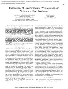
Figure 1. Grid and Uniform deployment topology (49 nodes) with the actual and estimated target trajectories.
without sensor coverage, we divided the area into a number of smaller cells of equal size (number of equal sized cells depends on the total number of nodes that are being deployed) and then randomly placed a node in each of the resulting cells. Figure 1 illustrates the grid and uniform deployment topologies with 49 nodes in the target area. We assume that each node is equipped with an acoustic sensor and that it samples the ambient sound at predefined intervals. We refer to these intervals as time steps in the rest of this report. In the simulator, we have modelled the acoustic samples measured by the sensors as a simple distance based function, wherein the intensity of these readings is an inverse function of the Euclidean distance between the current position of the target and the location of the sensors. The acoustic measurements recorded by the sensors are, therefore, not actual readings but rather synthetically generated based on the calibration results. For simplicity, we limit this work to estimation of a single target moving along a straight diagonal line from a point at the bottom left comer of the topology to the right hand top comer. The velocity of the target was set to 0.35m/sec and each simulation was run for 450 seconds. The base station is located at the centre of the topology (at location 60,60). The complete simulation consists of two parts. The first part is performed in NS2 where all the measurements during the simulation run are recorded by each node and then these measurements are forwarded to the centrally located base station, over multi-hop, where they act as inputs to the PF. The PF assumes the values ql = 0.002 and q2 = 10- 6 , in reference to (6), and low values for the birth and death probabilities, Pb = Pd = 0.01, in this case. Once all the data is available, the base station runs the PF code (offline, in MATLAB). The NS2 simulation setup parameters are listed in Table 1. Figure 1 shows the actual trajectory of the target and an example of the estimated track predicted by the PF for both
grid and DR deployment. As can be seen from this figure, the PF is very accurate in tracking the motion of the target. To quantitatively measure the performance of the tracking system, we define a metric, accuracy ofestimation as the average Euclidean distance between the actual and estimated location of the target. This metric is computed at each step of the execution of the PF. The second metric used in our evaluation is the computation time required for executing the PF algorithm. The total computation time is T comp = T ns + Tpf where T ns is time (real-time) taken in Ns2 to collect all the measurements at the base station for a particular run of simulation and Tp f denotes the time taken by MATLAB to run the PF at the base station. For each run of the simulation, the measurements were taken for each node at the sampling interval T. For each time step when the PF detects the presence of the target, the error is calculated in terms of the Euclidean distance between the estimated location as indicated by the PF and the actual target location. For each run of the simulation, we calculated the statistical mean and standard deviation of these errors. We repeated each of our simulations 100 times and the results are shown as an average result across all the runs including the standard deviation. A similar process is repeated for the second metric, the computation time.
4.1
Calibration
Calibration of the nodes is an important aspect of a realistic target tracking system. Referring to the mean of the measurement function (9), repeated here, dropping the time index for brevity -
Zi -
2
ai
+ "Ii Id-~ i ,
(21)
in order to accurately track a target there are two parameters which must be determined for each sensor i, that is the gain, "Ii and the noise variance, It is assumed that the other values, ~ and c from (10) are known, or can be calculated by a separate calibration mechanism, and are identical for each mote. We assume that a white noise source of unit (arbitrary) intensity is available, which can be placed at a unit distance from the sensor to be calibrated. We also assume that the resulting parameters are independent of the sensor orientation, which mayor may not be valid, depending on the sensor. From (21), if there is no signal from the source (1 = 0 or di ~ 00) then each measurement is solely from the noise,
a;.
167
Authorized licensed use limited to: IEEE Xplore. Downloaded on October 30, 2008 at 00:59 from IEEE Xplore. Restrictions apply.
Grid Deployment
Uniform Random Deployment
CompLtation Time -
Grid Dep!oymen1 roo - + - UnIfonn Random D&ployment
500
300
16 25
36
49
64
Number of Nodes
81
100
16 25
36
49
64
Number of Nodes
81
100
16
25
36
49
81
100
(c)
(b)
(a)
64
Number of Nodes
Figure 2. Effect of number of deployed nodes on the estimation error and computation time which encapsulates background noise and internal measurement noise. Thus, taking the mean of M o measurements ziO,m) from sensor i gives an estimate of
a;
Mo ,,2 _ _1_ "" (O,m) ai - M ~ zi .
°m=l
(22)
Similarly, if the source of unit acoustic power is placed at exactly unit distance from the sensor, then 21 reduces to (1)
Zi
2
= ai + 1i
(23)
these figures, for grid deployment the mean tracking error drops from about 5.3 meters for 16 nodes to 2.47 meters for 49 nodes. For DR deployment the corresponding decrease is from 5.37 meters to 2.45 meters. A high variation in mean and standard deviation is observed for DR deployment. This can be attributed to the random nature of the DR deployment strategy. For a fixed target trajectory, random placement of nodes results in more variation in tracking error across the simulation run as compared to the grid deployment. The DR deployment performs better or worse than the grid deployment depending on the node placement with respect to the target trajectory.
and so if M 1 measurements are taken, then the sample mean gives an estimate of 1i
%age Packet Lost --II- Grid Deploymen1
.......... Uniform Random Deployment 20
(24) For the simulations, gain and noise variations values are randomly selected for each mote. The gain is chosen between 1000 and 8000 and the noise variance between 5 and 40. The remaining parameters in the measurement model are chosen to be ~ = 2.2 (the path loss factor) and c = 1.5 (the measurement nonlinearity) as these values correspond well to the measurements taken in the calibration procedure before the experiments described in Section 6.
4.2
16
36
49
64
Num bar 01 No des
81
100
Figure 3. Effect of the number of nodes on packet loss.
Effect of the number of sensor nodes
To begin with, we focus our attention on evaluating the effect of the number of deployed sensor nodes on the aforementioned performance metrics. We increased the number of sensor nodes from 16 to 100 in a 120m x 120m area. Other important simulation parameters selected for this set of simulations include fixing the number of particles to 5000 and the sampling interval equal to 1 sec. Figures 2 (a,b) show the mean tracking error in the target's location for both grid and uniform random topologies. As can be seen from
25
The mean tracking error for both grid and DR deployment fluctuates in a very small band for any further increase in the number of the nodes beyond 49. However, if we look at Figure 2(c), which shows the computation time of the PF versus the number of deployed nodes, we can see that the computation time of the PF grows almost linearly with the number of deployed nodes for both grid and uniform random deployment. Packet loss also increase sharply with increase in number of nodes beyond 49 as shown in
168
Authorized licensed use limited to: IEEE Xplore. Downloaded on October 30, 2008 at 00:59 from IEEE Xplore. Restrictions apply.
Grid Deployment
Uniform Random Deployment
Computation Tme 350
...........
1K
2K
3K
4K 5K 6K 7K Number 01 Particles
8K
9K 10K
-
'-
-
-
- - - Grid Deploymerrt --+- Uniform Random Deployment
250 200
150
100'-------1-'--'---'--'---'--'--'---'---'------'
1K
2K
3K
4K 51< 6K 7K Number of Particles
(a)
6K
9K 10K
1K
2K
(b)
3K
4K 51< 6K 7K Number of Particles
6K
9K 10K
(c)
Figure 4. Effect of the number of generated particles on the estimation accuracy and computation time.
Figure 3. This suggests, that for the given size of the deployment field, target and sensor node characteristics (size, velocity, and intensity of target, and sensitivity of sensors etc.), and the selected networking and simulation parameters, the optimal density for the deployment of sensor nodes should be somewhere around 34 nodes per 100m2 , which corresponds to 49 nodes for the target area under investigation. This node density gives a balance between the error in estimation (mean tracking error of about 2.5m) and total computation time (about 230 seconds).
4.3
Effect of the number of generated particles
Next, we examined the effect of the number of generated particles on the performance of the tracking system. Recall that in our system, a number of particles are randomly generated near the sensor nodes. Further, the number of particles are independent of the number of deployed nodes (see Section 3) and only the Tpf component of the total computation time varies with change in number of particles. Figure 4 shows the results of the simulation for different number of generated particles for both grid and DR deployments. The number of nodes are 49 and the sampling interval is 1 sec. The error in estimation for grid deployment reduces from about 3.5 meters to 2.2 meters when the number of particles are increased from 1000 to 6000. After that the error begins to decrease at a much slower rate. For DR deployment, the mean tracking error reduces from 3.49 meters with 1000 particles to 2.45 meters at 5000 particles. However, from Figure 4(c) we can see that the computation time of the PF grows linearly with the number of generated particles. This suggests that given the simulation parameters, 5000-6000 particles is a good tradeoff between detection accuracy and computation time.
4.4
Effect of the sampling interval
Figure 5, shows the effect of the variation in sampling interval on the PF's behaviour. The number of nodes is set as 49 with 5000 particles. Intuitively, the larger the sampling interval, the longer the nodes will remain idle, hence the less energy that they will consume. However, as can be seen from this figure, the error in estimation of the target's location begins to increase with the increase in the sampling interval. Best tracking results are obtained with 0.5 to 1 sec sampling interval for both grid and DR deployment. The computation time, on the other hand, reduces from about 500 sec to 230 sec as the sampling interval is increased from 0.5 sec to 1 sec in Figure 5(c). This implies that given the node density and the selected simulation parameters, 1 sec sampling time is a sensible choice for this case.
5 Theoretical Analysis and Comparison In this section we first derive the Cramer-Rao Bound for the scenario used in our simulations. We next compare this theoretical lower-bound with the results from our simulations.
5.1
The Posterior (PCRB)
Cramer-Rao Bound
The Cramer-Rao Bound (CRB) is a theoretical construct, which specifies a lower bound on the second-order estimation error performance of any unbiased estimator [6]. We now proceed to compute this theoretical bound for the scenario used in our simulations (refer to Section 4 for details on the simulation scenario). The state evolution model and the measurement model are as described in Section 3 (see also [12] for further de-
169
Authorized licensed use limited to: IEEE Xplore. Downloaded on October 30, 2008 at 00:59 from IEEE Xplore. Restrictions apply.
Computation Tme
UR Deploymeri (49 Nodes, 5000 Particles)
Grid Deployment (49 Nodes, 5000 Partides) '0
___ Grid Deployment ~ Uniform
Random Deploymen1
'50
'00 50 OL--L..--L..--L..-'-----J'-----J~~~--------'--------'
o
,
2
3
4
5
6
7
sampling Interval (in sec)
8
9
10
"
_, L---L..-L..-L..-L..-'------J'------Jl..--Jl..--Jl..--J--'
o
,
2
3
4 5 6 7 8 sampling In1erval (in sec)
9
'0
,
"
2
3
4 5 6 7 8 sampling Interval (sec)
'0
(c)
(b)
(a)
9
Figure 5. Effect of sampling interval on estimation accuracy and computation time. tails). For simplicity we will limit our analysis to the single target case, although the multi-target CRB directly follows [13]. As in the case of the simulation scenario, a WSN composed of N = 49 acoustic sensor nodes is deployed in a two-dimensional region of size 120m x 120m. An unbiased estimate of the state vector Xt, based on ZI:t and the known distribution of the initial target state, p(Xo), is denoted by Xt, and its covariance matrix by Pt. The lower bound of Pt, referred to as the posterior CramerRao bound is expressed as follows [6]
Pt
===
0.6
E t:
= [F-
1
]T J t F-
1
+ L H'!+I,i R t-Jl,i Ht +1 ,i,
(26)
i-I
where it is assumed that Q is zero. Here Ht,i is the Jacobian of hi (Xt ) evaluated at the true value of X t
(Xi - Xt)~'iltd~ff-2 Ht,i
=
o
(Yi - Yt)~'Yiltd~ff-2
o
(27)
-e
0.3
0.2
0.' 50
'00
'50
200
250
Time (sec)
300
350
400
450
Figure 6. Comparison of CRB and simulation results.
once again evaluated at the true value of Xt. The terms in (27) and (28) are as defined in Section 3.
5.2
N
J t+ 1
0.5
~0.4
w
E {(Xt - Xt)(Xt - Xtflzl:t,p(Xo)} ~ Jt- 1
(25) The inequality in (25) implies that the difference Pt - Jt- 1 is a positive semi-definite matrix. Matrix Jt in Equation (25) is referred to as the information matrix and its inverse is the PCRB. For a deterministic nonlinear filtering problem specified by equations (1) and (11), the information matrix can be computed recursively as follows [1]
-CRLB -RMSError
0.7
Comparison of PCRB and Simulation Results
For the PCRB calculations the initial state vector was chosen as X o = [15
0.25
5
0.25
0.7]T
(29)
where the first and the third components are in meters, while the second and the fourth components are in meters/sec. For the purposes of this work the initial J 0 was approximated as a diagonal matrix with
'Yi dt,i
J0 1
= Po = diag([O.l
0.01]2). (30) The displayed error bounds are computed as follows:
and R~; is given by
0.05
0.1
0.05
(28) (31)
170
Authorized licensed use limited to: IEEE Xplore. Downloaded on October 30, 2008 at 00:59 from IEEE Xplore. Restrictions apply.
....
)(
~
Figure 9. Particle Filter Convergence Figure 7. Target and Experimental Setup 24
@
Acoustic Variance Vs Time (Route' ,2--'3, '4--23,24)
18
25
@
2D
@
@,
~.
IS'
15
~o
4000
5
@
3000
2000
'000
21
@
1 Figure 8. Acoustic Variance vs Time
2
@
I"
~1
~
where J t- 1 [1, 1] and Jt- 1 [3, 3] are the diagonal elements of the inverse of the information matrix corresponding to the x and y coordinates respectively. Next we compare the theoretical lower error bounds with the root-mean square (RMS) errors of the simulated PF. The number of particles used was 5000 and the PF was run 100 times for the bound comparison. Figure 6 illustrates that the simulated PF follows the general trend of the theoretical bound. We expect some mismatch between the filter performance and the bound due to the fact that the bound is a theoretically ideal quantity.
6 Initial Experiments In order to test the performance of the PF based tracking system in a real world environment, we have conducted some preliminary experiments. These experiments are also used to validate the simulation results. In this section we present our initial findings obtained from these experiments. Figure 7 shows the setup of our testbed. We used a prototype testbed consisting of twenty five of the Xbow MicaZ motes. These motes were programmed to perform high frequency sampling to measure the acoustic signals (at 5kHz) generated by the target (a remote controlled toy car). These MicaZ motes were deployed in a grid of size 2.5 meters x 2.5 meters (Figure 7) with 50cm grid spacing. A mote attached with a laptop was used as the data sink. The motes measure the acoustic signals and send a summary of the acoustic samples to the laptop (single hop communication), which executes the PF. The approximate speed of the target
18
1
22
@
17
@
'-2
(gI
7
@
Figure 10. Tracking Results was 0.03rn/sec. Time synchronisation among the motes was achieved by a Beeper mote broadcasting a beacon message every 0.5 seconds (sampling interval). On receiving a beacon, each mote starts sampling to collect 1000 discrete samples (taking 0.2s at 5kHz). To reduce the storage requirements at the motes, radio communications and the size of the data packets' motes only maintain summary statistics (sum and sum of squares) instead of the raw values. These summary statistics were then transferred during the next 0.3 seconds over the wireless link to the base station. Note that the sample variance can be easily calculated at the base station as we know the total number of samples, sum, and sum of squares of the samples, as shown (32) To ensure that all data packets are received at the base station, we incorporated an application level TDMA scheme to allocate discrete contention-free time slots to each mote for data transfer to the base station. The base station executes the PF with 5000 particles. Prior to running the experiments, the environmental path loss factor and the
171
Authorized licensed use limited to: IEEE Xplore. Downloaded on October 30, 2008 at 00:59 from IEEE Xplore. Restrictions apply.
standard deviation of the background noise are estimated by calibrating each mote carefully in the same experimental environment, as described in Section 4.1. Figure 8 shows the acoustic variance with time calculated at the base station for some of the deployed sensors. Figure 9 illustrates the two states of the PF, where the initial set of particles are shown searching for a new target on the left, and particles, after a number of measurements from the target, are shown on the right. Some of the tracking results are shown in Figure 10 where actual paths are shown in black arrows. The figures only show the qualitative performance of the WSN based tracking system. We have not used the quantitative metrics described in the simulation (Section 4) as fine-grained ground truth about the position of the target, both in time and space, was not available for error computation. The qualitative results demonstrate that the PF based estimator performs very well in tracking different trajectories of the target using real data collected by off-the shelf WSN devices.
7
cations.
[2] L. Gu, D. Jia, P. Vicaire, T. Yan, L. Luo, A. Tirumala, Q. Cao, T. He, J. A. Stankovic, T. Abdelzaher, and B. H. Krogh, "Lightweight detection and classification for wireless sensor networks in realistic environments," in Proceedings of ACM SenSys 2005, 2005, pp.205-217. [3] M. F. Duarte and Y. H. Hu, "Vehicle classification in distributed sensor networks," J. Parallel Distrib. Comput, vol. 64, no. 7,pp.826-838,2004. [4] Q. Wang, W. Chen, R. Zheng, K. Lee, and L. Sha, "Acoustic target tracking using tiny wireless sensor devices," in 2nd Inti. Conf. on Information Processing in Sensor Networks (IPSN03), 2003. [5] NS2, "Network http://www.isi.com/nsnam/ns/.
Acknowledgement This work is funded by the Defence Science and Technology Organisation (DSTO), Australia.
References [1] B. Ristic, S. Arulampalam, and N. Gordon, Beyond the Kalman Filter: Particle Filters for Tracking Appli-
simulator
2,"
[6] H. L. V. Trees, Detection, Estimation and Modulation Theory (Part I). John Wiley and Sons, 1968.
Conclusion and Future Work
In this paper we present a detailed simulation-based evaluation of the performance of a WSN tracking system, which employs the PF algorithm. We observed the effect of various network design parameters such as number of deployed nodes, number of particles, and sampling interval on the estimation accuracy and computation time of the tracking system. We found that, for the given Ns2 simulation parameters, the optimal deployment density is around 34 nodes per 100m2 , optimal number of generated particles is about 5000, and optimal sampling interval is 1 sec. These recommendations on the choice of network design parameters can be utilized to engineer a real WSN-based tracking solution. We also derived the theoretical lower bound, the CramerRao Bound (CRB) and demonstrated that the results from our simulations are comparable to the bound. We presented initial results on the performance of a prototype WSN tracking system with 25 sensor nodes. The PF based tracking system performs well in tracking targets performing different manoeuvres in the target area. We are currently conducting further experiments to test our system in real environments. Our future goals are to enable real-time distributed tracking of multiple targets and to incorporate a localisation algorithm in the tracking system.
Artech House, 2004.
[7] A. Ledeczi, A. Nadas, P. Volgyesi, G. Balogh, B. Kusy, J. Sallai, G. Pap, S. Dora, K. Molnar, M. Maroti, and G. Simon, "Countersniper system for urban warfare," ACM Transaction Sensor Networks, vol. l,no.2,pp. 153-177,2005. [8] T. He, S. Krishnamurthy, J. A. Stankovic, T. F. Abdelzaher, L. Luo, R. Stoleru, T. Yan, L. Gu, J. Hui, and B. Krogh, "An energy-efficient surveillance system using wireless sensor networks," in Proceedings ofACM Mobisys, 2004. [9] M. 1. Coates and G. lng, "Sensor network particle filters: motes as particles," in Proceedings of IEEE Workshop on Statistical Signal Processing, Bordeaux, France, 2005. [10] T. Schon, F. Gustafsson, and P.-J. Nordlund, "Marginalized particle filters for mixed linear/nonlinear state-space models," IEEE Trans. Signal Processing, 2005. [11] M. G. Rutten, N. J. Gordon, and S. Maskell, "Recursive track-before-detect with target amplitude fluctuations," lEE Proc.-Radar Sonar Navig., vol. 152, no. 5, pp. 345-352, Oct. 2005. [12] B. Ristic and S. Arulampalam, "Integrated detection and tracking of multiple objects with a sensor network," in Preprint. [13] B. Ristic and M. Morelande, "Cramer-rao bound for multiple target tracking using intencity measurments," in Conference on Information, Decision and Control (IDC 2007), Adelaide, Australia, Feb. 2007.
172
Authorized licensed use limited to: IEEE Xplore. Downloaded on October 30, 2008 at 00:59 from IEEE Xplore. Restrictions apply.