Dec 12, 1989 - cution of parallel and distributed programs as a framework for the .... itored for the performance analysis of data-driven opera- tions. A complete ...
I
IEEE TRANSACTIONS ON SOFTWARE ENGINEERING, VOL. 15, NO. 12, DECEMBER 1989
1615
Performance Measurement for Parallel and Distributed Programs: A Structured and Automatic Approach CUI-QING YANG
AND
BARTON P. MILLER,
MEMBER, IEEE
Abstract-This paper presents our new approaches in designing performance measurement systems for parallel and distributed programs. One of the approaches involves unifying performance information into a single, regular structure that reflects the structure of programs under measurement. We have defined a hierarchical model for the execution of parallel and distributed programs as a framework for the performance measurement. A complete picture of the program’s execution can be presented at different levels of detail in the hierarchy. The second approach is based upon the development of automatic guidance techniques that can direct users to the location of performance problems in the program. Guidance information from such techniques will supply not only facts about problems in the program, but also provide possible answers for the further improvement of program efficiency. A performance measurement system, called IPS, has been developed as a prototype of our model and design. IPS is implemented on the Charlotte distributed operating system at the University of Wisconsin-Madison. Some of the test results from IPS are also discussed in the paper to demonstrate unique features of our measurement system.
niques and tools are needed to aid in performance evaluation of parallel and distributed programs. Two gaps are observed in the current state of performance measurement tools for parallel and distributed programs. The first gap, the semantic gap, is a gap between the semantics of the structures with which we build parallel or distributed programs and the semantics by which performance measurement systems to view parallel or distributed programs. On the one hand, people are using more structured methods to develop parallel and distributed programs to cope with the increased complexity. Some examples of these methods are: new constructs in operating systems, a variety of parallel and distributed programming languages, and the current trend toward object-oriented distributed systems. On the other hand, most of the existing performance measurement systems for parallel and distributed programs are built without a welldefined model. Performance measurements in these sysIndex Terms-Critical path, distributed computing, hierarchical model, operation systems, parallel or distributed programs, perfortems were treated ad hoc. A few approaches have defined mance measurement. structures in measurement systems to model the structure of programs. However, many structures of such systems I. INTRODUCTION do not match the structure of programs seen by a programBUILDING performance measurement system for mer. This semantic gap prevents many measurement tools parallel and distributed programs involves the col- from capturing the infrastructure of programs and from lection, interpretation, and manifestation of information providing a complete picture of program’s execution. The second gap is called the functional gap. Users of concerning the interactions among concurrently executing processes. The inherent concurrency in a distributed pro- performance measurement tools want not only to know gram, the lack of total ordering for events on different how well their programs execute, but also to understand machines, and the nondeterministic communication delay why the performance may not be as good as expected. between peer processes in such a program add complexity The performance metrics provided by most measurement to the problem of performance measurement. The con- tools are good indications of what happened during a proventional methods of performance measurement for se- gram’s execution, but are of little use as guides to the quential programs are not adequate in the distributed en- improvement of program performance. A gap exists bevironment because they address only the performance of tween what users need and what measurement tools can individual programs on a single processor. New tech- offer. Users need more help from a measurement tool to locate the performance problems and to find ways for possible improvements. Manuscript received October 18, 1988; revised April 17, 1989. RecIn this paper, we present our new approach to bridge ommended by P. A. Ng. This work was supported in part by DARPA under Contract N00014-85-K-0788 and by the National Science Foundation unthese two gaps. The basis of our approach is to unify all der Grants MCS-8105904, and CCR-8703373 to the University of Wisconperformance information in a single, regular structure sin-Madison. which matches the structure of programs. Such a structure C.-Q. Yang is with the Department of Computer Science, University of North Texas, Denton, TX,76203. allows easy and intuitive access to performance informaB. P. Miller is with the Department of Computer Sciences, University tion, supports the construction of flexible user interfaces, of Wisconsin-Madison, Madison, WI 53706. and facilitates automatic reasoning about a program’s beIEEE Log Number 8931158.
A
0098-5589/89/1200-1615$01.00 0 1989 IEEE
1616
IEEE TRANSACTIONS ON SOFTWARE ENGINEERING, VOL. 15, NO. 12, DECEMBER 1989
havior. Our performance measurement tool also provides facilities that aid users in understanding program behavior and locating trouble spots. We have developed automatic guidance techniques, such as the critical path analysis for the execution of distributed programs, for locating performance problems in programs. These techniques not only supply facts about performance behavior of the program, but also provide possible reasons for the performance problems in the program. In the following discussion, we start with a brief overview of related research in Section 11. This provides a base line for the discussion of our new approach. Section I11 describes our hierarchical model for distributed programs and a corresponding model for program measurement. These models unify many levels of performance data and serve as the framework of the performance measurement system. Section IV discusses automatic guidance techniques for performance analysis of execution of distributed programs. The major design considerations and some implementation details of the measurement system, IPS, are presented in Section V. Section VI describes some measurement results using IPS to show the functions and features of the new measurement tool. We conclude our paper by summarizing the key ideas and discussing directions for future research in Section VII.
11. RELATEDRESEARCH Much of the research on performance measurement of distributed systems and programs shows that we can describe the behavior of a distributed program at many levels of detail and abstraction. Marathe classifies the performance parameters of a multiprocessor system along the “machine cycles” axis into four separate levels: system programming, operating system design, hardware architecture, and hardware engineering [24]. The same method of classification can also be used to study performance behavior of parallel and distributed programs. The two most common levels for describing performance of distributed programs are the intraprocess and interprocess levels. Traditional or intraprocess performance measurement tools provide information about individual process. The gprof facility on BSD Unix [ 141, the HP sampler/3000 [30], the Mesa Spy [25], and other tools [l 11, [17] are all based on the measurement of information about individual processes (such as subroutine call frequencies or memory access rates). Performance tools for distributed programs have concentrated on interactions between processes. There are two main reasons for looking at process interactions. First, process interactions are subject to synchronization problems such as race conditions and protocol mismatches. Second, many I/O operations such as file accesses in a distributed environment are mapped into interactions between server and client processes. Therefore, process interactions are traced to understand the state changes of process. Gertner [ 131 explicitly recognized the importance of
monitoring messages as interactions among processes. He models his performance evaluation tool after finite state machines and uses traces of the process interactions (messages) to trigger the state transitions. Similarly, in a case study of the performance measurement of a distributed dining philosophers algorithm on ZMOB [ 11, [34], messages between processors are assigned time values and recorded upon transmission, reception, or dequeueing for application input. Miller has developed a measurement tool for distributed programs (DPM) based solely on the interprocess level [26]. The system monitors program activities at the process level and communication events among different processes. Other than message communication, some measurement systems take various resources (e.g., CPU or memories) shared by processes as interactions among them. Performance measurement of EGPA processor array [12], [18] only traces the history of process identifiers which have run on the CPU. Nevertheless, the binding of switchable memory modules with processing elements in the system MIDAS [23] was monitored for the performance analysis of data-driven operations. A complete picture of program’s execution needs information from different levels and some way to coordinate the information received from these various levels of abstraction. Research on integrated instrumentation environment for multiprocessors [32] and the PIE project [15], [33] at CMU proposes the concept of programming observability. It requires provisions for observing status and performance events at all levels (hardware level, kernel level, run-time support level, and application level) and the combination of program run-time information and development-time information. The integrated view is important to the programmer’s ease in using the performance tool. The relational data model in the PIE project integrates various information at different levels and different stages of development. However, since the relational model does not fit the structure of programs, it is hard to have information from various levels form a coherent picture of a program’s execution. The structure of a measurement system needs to match the structure of programs to be measured. In this way, the so-called semantic gap will be reduced. The measurement results from most performance systems are presented in some form of performance metrics, such as the process execution time, message traffic statistics, and overall parallelism. These metrics are good for the evaluation of the performance outcome of a program’s execution. They tell much about how good or bad the program’s execution is but little about why. Few efforts were directed at the study of combining performance measurement tools with techniques to locate performance problems and improve the behavior of parallel and distributed programs. This leads to the so-called functional gap. A performance measurement tool should not only be a judge of the past, but also be a prophet of the future. Programmers need more than a tool that provides extensive lists of performance metrics; they need tools that will direct
I
YANG AND MILLER: PERFORMANCE MEASUREMENT FOR PARALLEL AND DISTRIBUTED PROGRAMS
them to the location of performance problems and give them guidance for possible solutions.
1617
whole program level
111. THE PROGRAM AND MEASUREMENT HIERARCHIES A general approach to problem-solving is to decompose a big problem into a set of smaller problems and first to solve these smaller problems. This decomposition is the way that we structure programs: the original problem is divided into pieces such-as modules and processes. Different data structures ani%individual procedures are further defined in each process. All of these objects form a hierarchy within the structure of the program. Our approach to the performance measurement of parallel and distributed programs is based on organizing the performance measurement tool as a regular structure that matches the structure of the program being measured. We choose a hierarchical model as a framework for our performance measurement system. A hierarchical model provides multiple levels of abstraction, supports multiple views, and has a regular structure. The performance information within this hierarchy reflects the program behavior based on its internal structure, and gives a complete picture of program's execution. An interactive user interface allows users to easily traverse through the hierarchy, to zoom-in/zoom-out at different levels of abstraction, and to focus on the places in the program structure that have great impact on the performance behavior of the program. In this section we demonstrate these ideas by presenting a sample hierarchy for distributed programs that is based on our initial implementation systems-the Charlotte Distributed Operating System [2] and 4.3 BSD Berkeley UNIX [20]. Both systems consist of processes communicating via messages. These processes execute on machines connected via high-speed local networks. The hierarchy presented here serves as a test example of our hierarchical model and reflects our current implementation [27]. The hierarchy is not fixed and it is easy to incorporate new features and other programming abstractions. For example, we can add the light-weight processes (processes in the same address space) from the LYNX parallel programming language [3 13 to our hierarchy with little effort. Our hierarchical structure could be also applied to systems such as HPC [19], which has a different notion of program structuring, or MIDAS 1231, which has a three-level programming hierarchy. A . The Program Hierarchy In our sample hierarchy, a program consists of parallel activities on several machines. Machines are each running several processes. A process itself consists of the sequential execution of procedures. An overview of our computation hierarchy is illustrated in Fig. 1. This hierarchy can be considered a subset of a larger hierarchy, extending upwards to include local and remote networks and downward to include machine instructions, microcode, and hardware gates.
machine level
process level
procedure level
Fig. 1 . Overview of computation hierarchy.
1 ) Program Level: This level is the top level of the hierarchy, and is the level in which the distributed system accounts for all the activities of the program on behalf of the user. At this level, we can view a distributed program as a black box to which a user feeds inputs and gets back outputs. The general behavior of the whole program, such as the total execution time is visible at this level; the underlying details of the program are hidden. 2) Machine Level: At the machine level, the program consists of multiple threads that run simultaneously on the individual machines of the system. We can record summary information for each machine, and the interactions (communications) between the different machines. All events from a single machine can be totally ordered since they reference the same physical clock. The machine level provides no details about the structure of activities within each machine. 3) Process Level: The process level represents a distributed program as a collection of communicating processes. At this level, we can view groups of processes that reside on the same machine, or we can ignore machine boundaries and view the computation as a single group of communicating processes. If we view a group of processes that reside on the same machine, we can study the effects of the processes competing for shared local resources (such as CPU and communication channels). We can compare intra- and inter-
I
1618
IEEE TRANSACTIONS ON SOFTWARE ENGINEERING, VOL. 15, NO. 12, DECEMBER 1989
machine communication levels. We can also view the entire process population and abstract the process’s behavior away from a particular machine assignment. 4) Procedure Level: At the procedure level, a distributed program is represented as a sequentially executed procedure-call chain for each process. Since the procedure is the basic unit supported by most high-level programming languages, this level can give us detailed information about the execution of the program. The procedure level activities within a process are totally ordered. The step from the process to the procedure level represents a large increase in the rate of component interactions, and a corresponding increase in the amount of information needed to record these interactions. Procedure calls typically occur at a much higher frequency than message transmissions. 5) Primitive Activity Level: The lowest level of the hierarchy is the collection of primitive activities that are detected to support our measurements. Our primitive activities include process blocking and unblocking by the scheduler, message send and receive, process creation and destruction, procedure entry and exit. Each event is associated with a probe in the operating system or programming language run-time that records the type of the event, machine, process, and procedure in which it occurred, a local time stamp, and event type dependent parameters. The events are listed in Table I.
B. The Measurement Hierarchy The program hierarchy provides a uniform framework for viewing the various levels of abstraction in a distributed program. If we wish to understand the performance of a distributed computation, we can observe its behavior at different levels of detail. We chose a measurement hierarchy whose levels correspond to the levels in our hierarchy of distributed programs. At each level of the hierarchy, we define performance metrics to describe the program’s execution. For example, we may be interested in parallelism at the program level, or in message frequencies at the process level. We can look at message frequencies between processes or between groups of processes on the same machine. This selective observation permits a user to focus on areas of interests without being overwhelmed by all of the details of other unrelated activities. The hierarchical structure matches the organization of a distributed computation and its associated performance data. Table I1 lists several of the performance metrics that can be calculated by the measurement system. Some of these metrics are appropriate for more than one level in the hierarchy, reflecting different levels of detail. Table I11 summarizes the use of these metrics at each level. The list in Table I1 is provided as an example of the type of metrics that can be calculated. A different model of parallel computation can define a different program hierarchy with its own set of metrics.
IV. AUTOMATIC GUIDANCE TECHNIQUES We base our performance system on the idea that it should provide answers, not just numbers. A performance system should be able to guide the programmer in locating performance problems and should help users improve program efficiency. In this section, we discuss some analysis techniques that support our approach. The execution of a parallel or distributed program can be quite complex. Often individual performance metrics do not reveal the cause of poor performance, because a sequence of activities, spanning several machines or processes, may be responsible for slow execution. Consider an example from traditional procedure profiling. We might discover a procedure in our program that is responsible for 90 percent of the execution time. We could hide this problem by splitting the procedure into 10 subprocedures, each responsible for 9 percent of execution time. For this reason, it is necessary to detect a situation in which cost is dispersed among several procedures, and across process and machine boundaries. There are other problems that are difficult to detect using simple performance metrics. It may be important to determine the effect of contention for resources. For example, the scheduling or planning of activities on different machines can have a great effect on the performance of the entire program [2 11. Another example is the problem caused by the execution pattern of a program changing over time. A parallel program may go through a period of intense interaction with little computation, then switch to a period of intense Computation with little interaction among its concurrent components. In such a case it will be difficult to understand the detailed behavior of the program by analyzing the program’s execution as a whole. Our strategy in designing a measurement system is to integrate automatic guidance techniques into such a system. Therefore, information from these techniques, such as that which concerns critical resource utilization, interaction and scheduling effects, and program time-phase behavior should be available to help users analyze a program’s execution. In our research, we have developed one of the techniques-critical path analysis for the execution of distributed programs [35]. A . Critical Path Analysis for Execution of Distributed Programs
Turnaround or completion time is an important performance measure for parallel programs. When turnaround time is used as the measure, speed is the major concern. One way to determine the cause of a program’s turnaround time is to find the event path in the execution history of the program that has the longest duration. This critical path [22] identifies where in the hierarchy we should focus our attention. As an example, Fig. 2 gives the execution history of a distributed program with three processes. This figure displays the program history at the process level, and the critical path (identified by the bold
I
YANG AND MILLER: PERFORMANCE MEASUREMENT FOR PARALLEL AND DISTRIBUTED PROGRAMS
Process creation tblork-cpu: Process block for CPU tblork-,yc: Process block fo synch. tmter: Procedure entry Message send call fend : Message send
Process termination
trfart:
,
1619
tunbloct-cpu: Process un-block for CPU tunblock-ryc: Process un-block for synch. tCdf:
t,cv-c,,,l: trcv :
Procedure exit Message receive call Message receive
TABLE I1 PERFORMANCE METRICS Np: Number of processes. N,: Number of machines. T : Total execution time. rep,,: Total CPU time. Twit: Total waiting time. Twit-cpu:Total CPU wait time (scheduler waits) R: Response ratio, T / Tcpu. L: Load factor, (Tcpu+ T,dt-,,,,) / TIP" P : Parallelism, Tepu1 T. p: Utilization, P 1 N, M,: Message traffc (bytes/=) C: Procedure call counter M,: Message traffic (msgs/sec) PR: Progress ratio, T,,, / Twait
R , L, p, M,,M,, and C are metrics which T , N,,,N,, Tcpu, T l ~ t ,Tmdt will be applied to different leve6of the measurement hierarchy (see Table 111).
Process 1
N." NP
I
I
Program Level
Machine Level
X X X
X X
Process Level I
I
I
Process 2
Process 3
Procedure Level I
X
I
Send
Fig. 2. Example of critical path at process level
line) readily shows us the parts of the program with the greatest effect on performance. We can view a distributed program as having the following characteristics: 1) It can be broken down into a number of separate activities. 2) The time required for each activity can be measured. 3) Some activities must be executed serially, while others may be carried out in parallel. 4) Each activity requires a combination of resources, e.g., CPU's, memory spaces, and I/O devices. There may be more than one feasible combination of resources for different activities, and each combination is likely to result in a different duration of execution. Based on these properties of a distributed program, we can use the critical path method (CPM) [9], [22] to analyze a program's execution. The technique used in our critical path analysis is based on the execution history of a program. We can find the path in the program's execution history that took the longest time to execute. Along
this path, we can identify the place(s) where the execution of the program took the longest time. The knowledge of this path and of the bottleneck(s) along it will help us focus on the performance problem.
B. Program Activity Graph To calculate critical paths for the execution of distributed programs, we first need to build graphs that represent program activities during the program's execution. We call these graphs program activity graphs (PAG's). A PAG is defined as a weighted and directed multigraph, that represents program activities and their precedence relationship during a program's execution. Each edge represents an activity, and its weight represents the duration of the activity. The vertices represent beginnings and endings of activities and are the events in the program (e.g., sendheceive and process creation/termination events). A dummy activity in a PAG is an edge with zero weight that represents only a precedence relationship and not any real
I
1620
IEEE TRANSACTIONS ON SOFTWARE ENGINEERING, VOL. 15, NO. 12. DECEMBER 1989
action in the program. More than one edge can exist between the same two vertices in a PAG. The critical path for the execution of a distributed program is defined as the longest weighted path in the program activity graph. The length of a critical path is the sum of the weights of edges on that path. A program activity graph is constructed from the data collected during a program’s execution. Two classes of activity considered in our model of distributed computation are computation and communication. For computation activity, basic PAG events are computation (process) creation and scheduling events. The communication events are based on the semantics of our target system. In Charlotte, the basic communication primitives are message Send/Rcv and message Wait system calls [2]. A Send/Rcv call issues a user communication request to the system and returns to the user process without blocking. A Wait call blocks the user process and waits for the completion of previously issued Send/Rcv activity. Corresponding to these system calls are four communication events defined in the PAG: send-call, rcv-call, waitsend, and wait-rcv. These primitive events allow us to model communication activities in a program. We show, in Fig. 3, a simple PAG for message send and receive activities in a program. The weights of message communication edges in Fig. 3 (tsend, trcv7 twait-send, and twait-rev)? represent the message delivery time for different activities. Message delivery time is different for local and remote messages, and is also affected by message length. A general formula for calculating message delivery times is: t=Tl T2 X L , where L is the message length, and TI and T2 are parameters of the operating system and the network. We have conducted a series of tests to measure values of these parameters for Charlotte. We calculated average TI and T2 for different message activities (intra- and intermachine sends and receives) by measuring the round trip times of intra- and intermachine messages for 10,000 messages, with message lengths from 0 to the Charlotte maximum packet size. These parameters are used to calculate the weight of edges when we construct PAG’s for application programs.
c
c
Fig. 3. Construction of simple program activity graph.
All of our algorithms for the longest path problem are variations of this method. We define a root vertex of a directed graph as a vertex in the graph that has only out-going edges, and a leaf vertex of a directed graph as a vertex in the graph that has only in-coming edges. A diffusing computation on a graph can be described as follows: From all root vertices in the graph, a computation (e.g., a labeling messaie) diffuses to all of its descendant vertices and continues diffusing until it reaches all leaf vertices in the graph.
We distinguish two variations of the diffusing computation: synchronous execution and asynchronous execution. In synchronous execution, a nonroot, nonleaf vertex will diffuse the computation to its descendant vertices only after it receives all computations diffused from all in-coming edges. In asynchronous execution, a nonroot, nonleaf vertex will diffuse the computation to its descendant vertices as soon as it receives a new computation from any one in-coming edge. Synchronous execution can deadlock in a graph with cycles. However, the computational complexity of synchronous execution is linear in the number of edges and vertices. On the other hand, asynchronous execution does not need explicit synchronization spots in its execution. Potentially, this will provide more concurrency for the computation in a distributed environment. 2) Test of Different Algorithms: We chose the PDM shortest-path algorithm as the basic for our implementation of centralized algorithm which are used for comparison with distributed algorithm [6]. An outline of the PDM C. Algorithms of Critical Path Analysis algorithm are given in Appendix 1. More detailed discusAn important side issue is how to compute the critical sion of the algorithm can be found in [6]. Our implemenpath information efficiently. After a PAG is created, the tation of the distributed longest path algorithm is based critical path is the longest path in the graph. Algorithms on Chandy and Misra’s distributed shortest path algorithm for finding such paths are well studied in graph theory. [4]. Every process represents a vertex in the graph in their Since all edges in a PAG represent a forward progression algorithm. However, we chose to represent a subgraph of time, no cycles can exist in the graph. To find the long- instead of a single vertex in each process because the est path in such graphs is a much simpler problem than in number of total processes in the Charlotte system is limgraphs with cycles. Also, most shortest path algorithms ited and we were testing with graphs having thousands of can be easily modified to find longest paths, because of vertices. The algorithm is implemented in such a way that the acyclic property of our graphs. Therefore, in the fol- there is a process for each subgraph, and each process has lowing discussion, we consider those shortest-path algo- a job queue for the diffusing computation (labeling the current longest length of the vertex). Messages are sent rithms to be applicable to our longest-path problem. 1 ) Diffusing Computation on Graphs: Diffusing com- between processes for diffusing computations across putation on a graph, proposed by Dijkstra and Scholten subgraphs (processes). Each process keeps individual [8], is a general method for solving many graph problems. message queues to its neighbor processes. An outline of
+
11
1
I
YANG AND MILLER: PERFORMANCE MEASUREMENT FOR PARALLEL AND DISTRIBUTED PROGRAMS
the two versions of the distributed algorithm appears in Appendix 2. A detailed discussion of the algorithm is given by Chandy and Misra [4]. We used two application programs to generate PAGs for testing the longest path algorithms. The total number of vertices in the graphs varies from a few thousand to more than 10,000. Application 1 is a master-slave structure, and Application 2 is a pipeline structure. Both programs have adjustable parameters. By varying these parameters, we vary the size of the problem and the size of generated PAG's. All of our tests were run on VAX-11/ 750 machines. The centralized algorithms ran under 4.3 BSD UNIX, and the distributed algorithms ran on the Charlotte distributed operating system [2]. 3) Discussion: Speed-up (S) and efficiency (E) are used to compare the performance of the distributed and centralized algorithms. Speed-up is defined as the ratio between the execution time of the centralized algorithm (T,) to the execution time of the distributed algorithm ( T d ) : S = T,/Td. Efficiency is defined as the ratio of the speed-up to the number of machines used in the algorithm: E = S / N . We used input graphs with different sizes and ran the centralized and distributed algorithms on up to 9 machines. Speed-up and efficiency were plotted against the number of machines. The results are shown in Figs. 4,5 , 6, and 7. We have observed a speed-up of almost 4 with 9 machines in synchronous execution of the distributed algorithm. The distributed algorithm with larger input graphs and more machines resulted in greater speed-up but less efficiency. The sequential nature of synchronous execution of diffusing computations determines that the computations in an individual machine have to wait for synchronization at each step of the diffusion. As a result, the overall concurrency in the algorithm is restricted, and the communication overhead with more machines offsets the gain of the speed-up. The complexity of the synchronous version of the diffusing algorithms is linear with respect to the number of vertices and edges in the graph, because the diffusing computations go through each edge and vertex exactly once. In asynchronous execution, at the worst case, the computation will be proportion to the total number of all possible paths from the source to each vertex in the graph. Asynchronous execution can increase concurrency in a distributed computation by generating more diffused computations in the job queue and releasing the synchronization requirements among executions. However, in this case we sacrifice economy of work because the asynchronous algorithm does less careful bookkeeping. Our test results indicate that the work in the asynchronous execution grows so fast that even a parallel algorithm is not viable. V. DESIGNA N D IMPLEMENTATION OF IPS TOOL MEASUREMENT We have implemented a pilot performance measurement system for distributed programs, IPS, based on our
1621
Speed-up APPLICAlION I
3.
21
I
0
I
lVl=10284
IVI=3014
1
I
.
2
.
.
3
4
1
7
5 6 Machine*
.
,
7
R
.
I
9
IC1
Fig. 4. Speed-up of distributed algorithm.
BIliciencv
0.5-
.
0
1
I
.
2
.
.
3
1
--
~
~
-:-*
lVl-4414 IVI=3014
,
.
,
.
.
5
6
7
8
9
.
IO
U hladtiner
Fig. 5 . Efficiency of distributed algorithm.
speed-up APPLICATION 2
I
2
3
4
5
6
n Machimes
7
8
9
IO
Fig. 6. Speed-up of distributed algorithm.
hierarchical measurement model. IPS operates in two separated phases-data collection and data analysis. During the first phase, the program is executed and trace data is collected. All necessary data are collected automatically
I
1622
IEEE TRANSACTIONS ON SOFTWARE ENGINEERING, VOL. 15, NO. 12, DECEMBER 1989 Efficiency
'h
04 I
APPUCATION 2
.
.
.
2
3
4
.
.
5 6 Y Muhiner
.
.
7
8
.
9
1
10
Fig. 7. Efficiency of distributed algorithm.
USER Fig. 8. Basic structure of measurement tool.
during the execution of the program. There is no mechanism provided (or needed) for the user to specify the data to be collected. During the second phase, programmers can interactively access the measurement results. This section describes the design and implementation of IPS on the Charlotte distributed operating system. A . The Charlotte Distributed Operating System The Charlotte operating system was used for the initial implementation of IPS. Charlotte is a message-based distributed operating system designed for the Crystal multicomputer network [7]. Crystal consists of 18 VAX-11I 750 node computers and several host computers connected with an 80MB/sec Pronet token ring [3]. The Charlotte kernel supports the basic interprocess communication mechanisms and process management services. Other service such as memory management, file server, name server, connection server, and command shell are provided by utility processes [2].
B. Basic Structure IPS consists of three major parts: agents, data pools, and analysts (see Fig. 8). Each of the three parts is distributed among the individual machines in the system. The agent is the collection of probes in the operating system kernel and the language run-time routines for collecting trace data when a predefined event happens. The data pool is a memory area in every machine for the storage of trace data and for caching intermediate results from the analyst. The analyst is a set of processes for analyzing the measurement results. There is one master analyst that provides an interface to the user and acts as a central coordinator to synthesize the data sent from the different slave analysts. The slave analysts reside on the individual machines for local analysis of the measurement data. In our scheme, the raw data is kept in the data pool on the same machine where the data was generated. Slave analysts exist on each machine, instead of a single global analyst. The local data collection and (partial) analysis has several advantages. Trace data are collected on the
11
machine where they were generated. Local storage of trace data should incur less measurement overhead than transmitting the traces to another machine. Sending a message between machines is a relatively expensive operation. Local data collection in IPS will use no network bandwidth and little CPU time. A second advantage to local data collection is that we can distribute the data analysis task among several slave analysts. Low level results can be processed in parallel at the individual machines and sent to the master analyst where the higher level results can be extracted. It is also possible to have the slaves cooperating in more complex ways to reduce intermachine message traffic during analyses (such as in the critical path analysis).
C. Data Collection Local data collection requires that each machine maintains sufficient buffer space for the trace data. The question arises whether we can store enough data for a reasonable analysis. Procedure call events happen at a much higher frequency than interprocess (message) events. Event tracing for procedure calls could produce an overwhelming amount of data. We have measured the message and procedure call frequencies of several programs running on the Charlotte and Unix operating systems. The procedure call rates are over 6000 /second-almost three orders of magnitude greater than interprocess events [27]. Due to this high frequency, we use a sampling mechanism combined with modifying the procedure entry and exit code. Because we are using sampling at the procedure level, results at this level will be approximate. Sampling techniques have been used successfully in several measurement tools for sequential programs, such as the XEROX Spy [25] and HP Sampler/3000 [30]. We set a rate, ranging from 5-100 ms, to sample and record the current program counter (therefore the current running procedure). We also keep a call counter for each procedure in the program [14]. Each time the program enters a procedure, the counter of that procedure is incre-
I1 I
YANG AND MILLER: PERFORMANCE MEASUREMENT FOR PARALLEL AND DISTRIBUTED PROGRAMS
mented. At the sampling time, a record which includes a time stamp, the current procedure PC, and the procedure call counter is saved in the trace data. The sampling frequency can be varied for each program execution. A higher sampling rate will give better precision to the sample results. However, the sampling overhead also increases with the sampling frequency. Data gathering for interprocess events is done by agents in the Charlotte kernel. Each time that an activity occurs (most appear as system calls), the agent in the kernel will gather related data in an event record and store it in the data pool buffer. Our implementation for data collection stops at the procedure level, although the hierarchical model itself can be easily extended to include low level information such as that of per statement or per instruction execution. However, the huge amount of data involved in such low level activities prevents any simple solution. Our data collection facility also supports a multiprogramming environment. Processes under monitoring need first to register to the system (via a system call), and only those processes which have registered are under consideration for data collection.
1623
involve only table searching in master or slave analysts, whereas, queries in the third category are much more expensive due to processing of the large amount of raw data. The choice of data stored in IRT’s can have a large affect on the costs of user query processing. Most user queries fall into the first two categories; however, users may occasionally need direct access to the trace data. One such example is when the needed information is not provided by the metrics, e.g., the communication patterns among different processes. Another example is when a user needs to scrutinize the details about program’s execution, e.g., to check why a process is blocked during a given time period. These queries will fall into the third category and involve extra costs for processing the raw data. The metric information about the process and procedure levels is preprocessed by slave analysts and kept in local IRT’s. The metric information about the program and machine levels is preprocessed by the master analyst based on low-level information sent from all slave analysts and saved in IRT’s at the master analyst. The master analyst gets queries from the user and decides how to distribute a query among slave analysts. The query processing here is similar to the query processing in a distributed database D . Data Analysis system. The general structure for data analysis in our measureThe calcilation of performance metrics in the IPS dement tool is shown in Fig. 9. Analysis programs in the pends upon the ordering of different events in the system. master and slave analysts cooperate to summarize the raw For most metrics, the mdering only involves events ocdata in response to user queries. The master analyst can curring in the same machine (e.g., metrics for individual reside on any machine as long as communication channels machine and process). For other analysis (such as the critbetween master and slave analysts can be established. In ical path analysis in Section IV), we need information our implementation, the master analyst is a process run- about partial ordering among events in different maning on a host UNIX system. An independent user inter- chines. Only a few metrics depend upon the information face is separated from the implementation of the master of total ordering among events across machines. One such analyst, so that different interfaces between the user and example arise when calculating the elapsed time of the the master analyst can be adopted for different environ- whole program. Maintaining total ordering among events ments. in a distributed environment requires synchronizing clocks Since the amount of the trace data is usually quite big, on different machines. In our implementation, we adopted it is too expensive to process all user queries directly from a simple approximation method based on the TEMPO althose data. We create a set of intermediate result tables gorithm [16]. (IRT) in master and slave analysts to store information preprocessed from the trace data. VI. MEASUREMENT TESTSWITH IPS There are three different query processing categories. The IPS measurement system provides a wide range of The first category contains queries that only need the information in the IRT at master analyst. The master analyst performance information about a program’s execution. can easily handle these queries by accessing appropriate This information includes performance metrics at differentries in the IRT. The second category contains queries ent levels of detail, histograms of the basic metrics, and that require intermediate results stored in the IRT’s at guidance information for the critical path in a program’s slave analysts. The master analyst has to communicate execution. In evaluating the usefulness of our system, we with corresponding slave analysts to retrieve information have been able to obtain some interesting results in the in the IRT’s of slave analysts. The last category of user studies we have performed. More time is needed, howqueries needs direct access to the raw data of the slave ever, to fully evaluate the models, methods, and tools analysts, e.g., a query for a list of the event traces in presented in this paper. This section describes a sample certain time interval. User queries in this category will performance measurement session of a distributed applicause the trace data to be scanned at the time of the query cation to show the effectiveness of the information provided by the IPS, and to show how this information helps processing. The processing costs for queries in various categories us to better understand the performance behavior of a prodiffer significantly. Queries in first and second categories gram.
1624
IEEE TRANSACTIONS ON SOFTWARE ENGINEERING, VOL. 15, NO. 12, DECEMBER 1989
1
1-- --
-1-
I
I
I
I
I
I
I
I
I
I
I
I I
I
I. I
.I I
I
I
I
I
I
I
I
I
Fig. 9. General structure for measurement results analysis.
A . Interactive Measurement Session The program we have chosen for measurement tests on the IPS system is an implementation of the Simplex method for linear programming [ 5 ] . The configuration for our test is set as follows: the input matrix size is 36 x 36, the program has a controller process and 8 calculator processes, and these processes run on 3 node machines. IPS provides an interactive user interface for the measurement of programs. The interface supports a command menu from which users can choose appropriate actions. The menu contains two groups of commands. One group includes the commands for.maneuvering through different levels of the hierarchy-for example, going up one level, going down one level, and selecting other items in the same level. Another group consists of the commands for selecting different measurement actions, such as presenting metrics and displaying histograms and critical path information. The measurement session starts at the program level. We can select a command from the menu to display performance information at this level. Fig. 10 shows the metr i c ~at the program level. These metrics are defined in Section 111-B, and reflect various aspects of the performance behavior of the program. The information found in various histograms can help users investigate a program's behavior during a stretch of time. Fig. 11 shows a histogram of CPU time at the program level. The performance information at the program level gives us a general characterization of the program's execution. For example, as we can see from Fig. 10, the total message waiting time (Block-sync Time) for the entire program is large, and the overall parallelism (speed-up) un-
Metrics for Program Level
# of Machines: # of Processes: Elapsed T h e (ms): CPUTime(ms): Block-sync Time(ms): Block-cpu Tme(ms): Message Traffic(#): Message TraKic(bytes): # of Procedure: # of Procedure Calls: P~wdlelisni: Load Factor:
3 9
27670 31870 203794 9679 687 2220080 58 938 1.15
1.30
Fig. 10. Metrics at program level.
L 25
0
5
10 15 20 Elapscd Time (seconds)
Fig. 1 1 . Histogram of CPU time at program level.
der this configuration is only 1.15. These results raise questions about why the speed-up of the program's execution is so limited and where the bottlenecks in the program might be. For more detailed information, we continue our study at the machine and process levels. Fig. 12 shows the metrics at the machine level. Each machine has 3 processes.
YANG AND MILLER: PERFORMANCE MEASUREMENT FOR PARALLEL AND DISTRIBUTED PROGRAMS
Metricr
# of Process:’ Elapsed Time(=): CPU Time(ms): Block-sync Time(=): Block-cpu Time(=): Message Tr&c( #): Meaaage Tr&c(bytes): # of Procednns: # of Procedure Calls: Utilisation: Load Factor:
Machine1 3 27636 16233 58507 7273 429 1383104 22 626 0.59 1.45
Machinef 3 27541 7911 72911 1034 129 418488 18 156 0.28
1.13
Machine) 3 27500 7726 72376 1372 129 418488 18 156 0.28 1.17
Metrics Process Name: Elapsed Tme(ms): CPUTime(ms): Block-sync Time(ms): Block-cpu Time(ms): MeMage Traffic(#): Measage Traffc(bytes): # of Procedures: # of Procedure Calls: Response Ratio: Load Factor:
1625 Process S control[ll 27240 9988 12230 5022 343 1104112 10 522 2.60 1.50
Process 4 calcs[3] 27352 3187 22911 1254 43 139496
Process 6 calcs[6] 27421 3058 23366 997 43 139496
6
6
52 8.55 1.39
52 8.55 1.32
Fig. 12. Metrics at machine level.
Fig. 13. Metrics at process level (in Machine 1).
However, Machine 1 has performance results different from those of Machines 2 and 3. This is because Machine 1 runs with the controller process and 2 calculator processes, whereas Machines 2 and 3 run with three calculator processes each. The process level information of machine 1 is shown in Fig. 13. Two calculator processes (processes 4 and 5) in machine 1 have similar performance behavior. All other processes in machines 2 and 3 are calculator processes and have similar performance results as in machine 1. We can also check histograms of the different metrics at machine and process levels. We can go further, to the procedure level, to investigate the behavior within each process. Fig. 14 shows this information for the controller and one of the calculator processes. The profiling information here is presented in the same format as in conventional profiling tools [25], [30]. The information about the distribution of CPU time in different procedures can help users determine which part of the program code dominates the execution.
program level. We can see that the communication cost (including intermachine and intramachine messages) is more than one third of the total length of the critical path. This reflects the fact that the communication overhead in Charlotte is relatively high compared to other systems [2]. The critical path information at the process level (see Fig. 16) gives us more details about the program’s execution. The execution of the controller process takes 58 percent of the whole length of the critical path, while the execution of all calculator processes take less than 5 percent of the whole length. The ratio between the execution of controller process and all calculator processes in the critical path is more than 10 : 1, whereas the measurement result in Section VI-A indicates that the ratio between the execution of controller and each calculator is only about 3 : 1. Therefore the critical path information shows more clearly the domination of the execution of the controller process. Such domination of the controller in the critical path restricts the overall concurrency of the program. This explains why the parallelism for the current configuration is so low. From the length of the critical path, we can calculate the maximum parallelism of the program [lo], [28], which equals the ratio between the total CPU time and the length of the critical path. This maximum parallelism depends upon the structure and the interactions among the different parts of the program. The maximum parallelism for the program under our tests (with 8 calculators running on 3 machines) is only l .91. The communication costs and the CPU load effects in different machines lower the real parallelism to l . 15. Finally, we display critical path information at the procedure level in Fig. 17. This information can be useful in locating performance problems across machine and process boundaries. The top three procedures, that take 49 percent of the entire length of the critical path, are in the controller process. Procedure MainLoop in the calculator processes, which is in charge of communications between calculators and the controller, takes 33 percent of the entire execution time of each calculator process (see Fig. 14). However, they are much less noticeable in the critical path because of the dominance of the controller process.
B. Information from Critical Path Analysis The information from various metrics and histograms gives us a general picture of the program’s execution. We have learned about many aspects of the program’s behavior from this information; for instance, that parallelism of the program is not high, that there is considerable communication between the controller and calculator processes, and that each calculator process has light work load and spends most of the time in waiting for messages. Howeb-er, all this information is .mainly applicable to individual activity in the program. It tells us little about the interactions among different parts of a program, and about how these interactions affect the overall behavior of a program’s execution. Therefore, it is still difficult to discover why the parallelism is low, how much communications affect the program’s execution, and which process (controller or calculator) has a bigger impact on the program’s behavior. More sophisticated analysis techniques are needed for a measurement system that will help users in analyzing performance results. The critical path analysis technique in IPS provides guidance for finding possible bottlenecks in a program’s execution. The critical path information is represented by the percentages of communication and CPU time of the various parts of the program along the total length of the path. Fig. 15 gives the critical path information at the
C. Remarks We have seen that the execution of the controller process dominates the performance behavior. This is be-
1626
IEEE TRANSACTIONS ON SOFTWARE ENGINEERING, VOL. 15, NO. 12, DECEMBER 1989
ProcedureNuoe MainLool, Init Sendchi madl CheckWaItig
Counter
Time(%)
1
44
PeCV
main Getarg s&uD ConvertNum
3 304
Totd
dorowop Mainhp selecttherow Idid setup main
15 1 15 1 1 1
50
Total
34
100
33
10 1
* 100
(a) Contr6lle.r
(* denotes 1-
than 1%)
Fig. 14. Execution profiling of controller and calculator.
Inter-machine Msg Intra-madiie Mag
Totd
I Mainhp 1360 16667
100
Fig. 15. Critical path information at program level.
P(1,3) CPU P(1,3)->P(3,5) Msg P(3,5)->P(1,3) Msg P(1,3)->P(2,5) Msg P(2,5)->P(1,3) Mag P(3,4)->P(1,3) Msg P(lJ)->P(3,4) Mag P(1,3)->P(2,4) Mag P(2,4)->P(1,3) Msg P(1,3)->P(1,5) M.g P(1,5)->P(1,3) Msg P( 1,3)->P( 1,4) Msg P(l,4)->P(ls3)Msg P(1,3)->P(3,3) Msg P(3,3)->P(1,3) Msg P(3,5) CPU P(1,5) CPU P(2,5) CPU P(3,4) CPU P(2,4) CPU P(1.4) CPU pi3;3j CPU Total
(Mach1, Roc 3) (Mach 1, Roc 3) (Mach 1, Roc 3)
Scndchid
9740
58 840 5 8 4 0 5 480 3
4 8 0 3 4 8 0 3 480 3 4 4 0 3 4 4 0 3 4 0 8 2 4 0 8 2
272 272 240
2 2 I
2 4 0 1
159 8
8
I I 1
7
9
4
4
4
loo 67 0
42 l a 7
* lo(
(P(i,j) denotes p r o c e ~j ~ in machinei, denoted less than 1%) Fig. 16. Critical path infomation at process level.
cause, in our test configuration, the controller process serves too many (8) calculator processes, but each calculator process is lightly loaded. One way to cope with the problem is to reduce the number of calculator processes in the program. We have conducted a set of measurement tests with programs having 2 to 8 calculator processes for the same 36 X 36 input matrix, running on 3 machines. The test results are shown in Fig. 18(a). We can observe that, to a certain extent, for this fixed initial problem, having fewer calculator processes gives a better result. The execution time has its minimum when the program runs with 3 calculators. However, if the number of calculator processes gets too small (2 in this case), each
Checkwaiting Mainhp Mainhp Mainhp Mainhp Mainhp
21 17
I
(Machl, Proc 3) (Mach1, Roc 3) (Mach 3, Proc 4) (Mach 1, Proc 3) (Mach 3, Proc 5) (Mach 1, Proe 5) (Mach2, Roc 4) (Mach 1, Proc 4) (Mach 2, Roc 5) 02
Totd CPU (* den& h..than 1%)
Fig. 17. Critical path information at procedure level.
calculator has to do too much work and creates a bottleneck. Note that the test using 2 calculator processes is the best with respect to the assignment of processes to machines (only one process per machine). While in the 3 calculator case the controller process is running on the same machine as a calculator process. Therefore, the contention for CPU time among processes is not the major factor that affects the overall execution time of the program. The critical path information for these tests (shown in Fig. 18(b)) supports our observation. For the configuration of 3 calculator processes, the controller and calculator process have the best balanced processing loads, and the lowest message overhead. This coincides with the shortest execution time in Fig. 18(a). The Simplex program has a master-slave structure. The ratio between computation times for the controller and calculator processes on the criticaE path reflects the balancing of the processing loads between the master and slaves in the program. We have observed that when the master and slave processes have evenly distributed processing loads (dynamically, not statically), the program shows the best turnaround time. Otherwise, if the master process dominates the processing, the performance suffers due to the serial execution of the master process. On the other hand, if the slave processes dominated, it would be possible to add more slaves. Appendix 3 contains a proof that supports our claim that for programs with the master-slave struc-
YANG AND MILLER: PERFORMANCE MEASUREMENT FOR PARALLEL AND DISTRIBUTED PROGRAMS
1627
# Calculator Procwes (a) Fig. 18. Program elapsed time and components of the critical path. (a) Elapsed time. (b) Critical path components.
ture, the length of the critical path in the program's execution is at its minimum when the path length is evenly distributed between master and slave processes. The measurement tests given here shows that the data of the critical path provides extra information for the evaluation and analysis of program's behavior in their execution. This information can be used as guidance to adjust the structure of the program for better performance. Such adjustment involves, e.g., restructuring (decomposing or combining) individual processes in the program, regrouping or replacement of processes on different processors and rearranging procedures or even statements in a process, etc. Nevertheless, because of the inherent complexity with a parallel or distributed program, such restructuring will not be an easy job, and could be application dependent. Much more study needs to be done in respect to the future direction of automatic guidance techniques for the performance measurement of parallel and distributed programs. VII. CONCLUSIONS We have described a structured and automatic approach to the design and implementation of a performance measurement system for parallel and distributed systems. This approach is based on a hierarchical model as a framework for the measurement system and the integration of the traditional performance metrics with automatic guidance techniques. A prototype, the IPS system, based . on our approach has been built on the Charlotte distributed system. Experiments in measuring real application programs on IPS demonstrate that our measurement hierarchy intuitively maps performance information to the program's structure, and gives a multilevel view of the behavior of a program's execution. The abstraction of the hierarchy helps users easily focus on places of interest, while the technique of critical path analysis provides extra information.for performance debugging and directs users to possible bottlenecks in the program.
~
TI
for all U in G do DIU]:= 0; end
forall U in G do Com"&= #of in-coming edges;
initialize Q to contain SOURCE only; while Q is not empty do delete 9's head vertex U ' for each edge (U,.) siarting at U do ifD[v]< DIU]+ wur then
iz "I
Dv - D u ] + w ' PP1 if U waa never in g'then insert U at the tail of Q ; else insert U at the head of Q ;
end end end end
-
D[u] .end Q to contain 'hitialiie SOURCE only; while Q is not em ty do delete 9's hezwfvertex U; for each edge (U,.) starting at U do dec(Count rn . ifD U ] D\uy; wue then
Lv
:=U'
D\v\ := DIU]+ wu,; end ifComt[w]= 0 then insert U at the tail of Q ; end end end
1
-
I
1628
IEEE TRANSACTIONS ON SOFTWARE ENGINEERING, VOL. 15, NO. 12, DECEMBER 1989
APPENDIX 2 DISTRIBUTED ALGORITHM FOR CRITICAL PATHANALYSIS The following is a sketch of the distributed algorithm for critical path analysis (see Section IV): U in sub-graph G do Couutu[u]:= # of insoming edges; DIU] := 0;
for d U in sub-graph G do Countcr[u] := 0; Dlul:= 0;
for d
end
md
initialise Q to include SOURCE or empty; rhik not termination do rhik Q inot empty a d mag queua noI hU do dekte h c d element; fekment = (Length.Pred) thm ifDIu] < Length thm if Counterlu] > 0 thm put Act[P[u]]in Q or mag queue;
initialise to include SOURCE or empty; while not local-turnination do while m not empty and m g queua not full do dekk Q’s head: (Length,Pred); dec(Countcr[u 1); i f D [ u ] < Length then PIU] := Bed; D[u[ := Length;
4 0
0’.
end
end
PIU1 := Pred; DIU] := Length; for each edge (U,.) U do
put kngth mag: (D[uI+wm~,Pred=U)in a msg queue for U ; md
caunter[u]
Q
+= x 0fo.t-gOkg
md end Send d mag queu- that are not empty;
edw;
f(laanter[u] = 0 thm put A&[P[u[] in Q a mag queue;
process is serialized with the concurrent execution of N slave processes. Hence, the length of the critical path in the program’s execution, L, ( N ), is:
h e h e fmm d neighbor procaul; if get any msg fmm other pmthen pmessing m g and put Length mag in Q ;
end
rlu put Ack(Pned]in
Fig. 19. Processes of master-slave structure.
fCoonter[u] = 0 t h m for each edge (U ,U) that atart. at U do pot k n g h mag: (D[u[+wu.,Pred=u) in Q a mag queue fo U; end
that starb at
Q or m g queue;
end end
end elle
CS += Nc, + -. N N C S
To find the minimum of L, ( N ), we have:
exchange m g with neighbaa to get consensus of global-termination
dec(:(Coonter[u]); YCounterluJ = 0 then pot Ack(P[ul]in Q a m g queue;
L c ( N ) = C,
md md md h d d mag queoa that are not empty; &e&e from .Uneigh& pmessa; if get any m g from other p m m then
and
processing mag and put length mag
N = E .
mdachinQ; md end
a,
(b):Sprhmnoua Veraion
(a): AspLhmnaus Vmion
APPENDIX 3 A PROOFOF THE MINIMUMCRITICAL PATHLENGTH In the following discussion, we give a simple proof to support our claim that for programs with the master-slave structure, the length of the critical path in the program’s execution reaches the minimum when the whole path length is evenly distributed between master and slave processes. Our proof applies the related study in Mohan’s thesis [29] to the aspect of critical path length. Assume that a general master-slave structure is represented as N slave processis working synchronously under the control of a master process (see Fig. 19). Let a computation have a total computing time of C, consisting of the time for master C, and the time for slaves Cs(for simplicity, all times are deterministic). The computation time in the master process includes one part for a fixed processing time (e.g., initialization, result reporting time) F, and another part of per slave service time (e.g., job allocating, partial results collecting) c,. Therefore,
C,
=
Nc,
+ F,.
Assume F, is negligible compared to Nc,, i.e., F, Nc,; we have:
C,