McGurrin Greczner
1 2 3
Performance Metrics: Calculating Accessibility Using Open Source Software and Open Data
4 5 6 7 8 9 10 11 12 13 14 15 16 17 18 19 20
Michael F. McGurrin (corresponding author) Noblis, Inc. 600 Maryland Ave., SW, Suite 755 Washington, DC 20024
21
5,150 words
22
5 figures
23
1 table
202-863-2974 (voice) 202-863-2988 (fax)
[email protected] David J. Greczner Noblis, Inc. 3150 Fairview Park Drive Falls Church, VA 22042 (703) 610-1808 (voice)
[email protected] Submitted on July 31, 2010
1
McGurrin Greczner
2
1 2 3 4 5 6 7 8 9 10 11 12 13 14 15 16
ABSTRACT
17 18 19 20 21 22
This type of analysis has previously been conducted primarily by metropolitan planning organizations or a few academic researchers. This new approach opens the door to much broader use. The approach was first developed and tested using data for the city of Washington, DC, and then for the city of Seattle, WA and some surrounding areas, including ferry routes. This new approach using free and open data and tools opens up accessibility analysis to a much broader array of stakeholders, including technically savvy users in the general public.
A new approach for calculating accessibility via both transit and automobiles is presented. Accessibility can be defined as the ability to reach desired goods, services, activities, and destinations. It is an important quantitative transportation performance measure that can be used as one objective measure of livability, a concept which has recently taken on increasing importance. This new approach leverages the parallel growth of open government data and free and open source software to provide a simple, flexible, low-cost method for conducting such analyses. In addition to data provided by the typical transportation planning process, such as traffic analysis zone boundaries and socio-economic data, this approach combines transit schedules published in the standardized General Transit Feed Specification format with map data taken from either TIGER files or the OpenStreetMaps Initiative. The tools used for calculating the accessibility measures are built around the OpenTripPlanner software. The outputs of the analyses include opportunity and gravity model accessibility indices, and estimates of the modal accessibility gap by traffic analysis zone. The process can be used to calculate both origin and destination based accessibilities (destination based journey to work trips were used in the proof-of-concept tests). In addition, geographic visualizations including travel time isochrones by mode, accessibility heat maps, and 3D visualizations combining geographic, accessibility, and demographic data were created.
McGurrin Greczner 1 2 3 4 5 6 7 8 9 10 11 12 13 14 15 16 17 18 19 20 21 22 23 24 25 26 27 28 29 30 31 32 33 34 35 36 37 38 39 40 41
3
There is a broad-based groundswell of support towards performance-based investments in and management of surface transportation systems (1-3). The U.S. DOT has cited six areas of interest (3): Safety Pavement and bridge condition Congestion Freight Environment/climate change Livability Some of these, such as safety and pavement conditions, are well understood and have long-established metrics for assessing performance. Others, such as livability, are new and can be difficult both to define and measure. One component of livability has been defined as “provide more transportation choices” (4). Accessibility metrics can be used to provide useful, quantifiable, and readily understood aggregate measure of meaningful choices by measuring the ability of citizens to access jobs, goods, and recreational opportunities using various transportation modes. The concept of accessibility is easily understood in general terms, but it is difficult to precisely define and measure it (5). One definition is “the ease of reaching goods, services, activities and destinations, which together are called opportunities” (6). Access can be viewed as the ultimate goal of transportation, since movement of people or goods an end in and of itself (7). Four factors affect accessibility: mobility, mobility substitutes (e.g., telecommuting), transportation system connectivity (the directness and degree of connectivity of the components of the transportation system) and land use, since physical proximity typically increases accessibility (7). Accessibility is a powerful concept for use in transportation planning, as it does not depend on the mechanisms used to achieve it. This allows alternative approaches to be considered on an equal footing with one another. For example, improved access to jobs may be provided by reducing congestion, growing the transit network, locating housing closer to work opportunities, or increasing the opportunities for telecommuting. As such, accessibility metrics provide a valuable complement to mobility and congestion metrics, such as average travel speed or delay. Pratt and Lomax state that “By using door-todoor travel time as the time measure, accessibility via alternative modes can be put on an essentially equal footing, as long as it is recognized that acceptability varies by mode. It is apparently as close to an ideal measure for multimodal performance analysis as can be achieved from the user perspective” (8). Transportation is rarely a goal in and of itself. It is a derived demand (9), meaning that the need for transportation is created by the requirement to fulfill some other demand, such as supplying goods or services, access to jobs, or to reach a vacation destination. Overly simplistic goals, taken alone, such as reducing vehicle miles traveled therefore run the risk of negative unintended consequences, such as reducing access to jobs, reducing access to goods, and negatively affecting the economy. When setting performance goals for transportation, it is important to examine the impact that the goal will have on the elements that created the original demand. Accessibility metrics can play an important role, since the ideal outcomes would maintain or increase accessibility while reducing the negative effects of transportation. Therefore, new techniques lowering the barriers to calculating accessibility have significant value.
McGurrin Greczner 1 2 3 4 5 6 7 8 9 10 11 12 13 14 15 16 17 18 19 20 21 22 23 24 25 26 27 28 29 30 31 32 33 34 35 36
37 38 39 40 41 42
4
Background and Measures of Accessibility There are many measures of accessibility. Handy and Neimeier (10) provide a review of accessibility in planning, and El-Geneidy and Levinson (11) provide a comprehensive, up-to-date review. This study utilized two types of models: cumulative opportunity and a gravity model. Cumulative Opportunity: Ci = ∑ Oj Bj Ci Oj Bj
Opportunities (jobs in this study) reachable from zone i Opportunities (jobs) at zone j A binary value equal to 1 if zone j is reachable within a predetermined time from zone I, otherwise equal to 0 This measures the number of jobs available to the residents of a given TAZ within a given transportation time. It has the advantages of being both simple to calculate and easy to understand. The units are number of jobs. However, the function uses a step function: all jobs within the travel time limit are counted equally, regardless of how quickly they can be reached, and jobs just one minute beyond the travel time limit are not counted at all. The gravity model addresses these limitations. Gravity Model:
Ai Oj Cij
Accessibility at a given zone, i Opportunities, in this case jobs, at a particular zone, j The time the mode of transit took to get from TAZ i to TAZ j
A downside of the gravity model is that it yields a unitless index whose only meaning is as a measure of relative value. Modal Accessibility Gap: In addition, the Modal Accessibility Gap (MAG) index between transit and automotive accessibility (12) is also calculated:
Ap Ac
Transit Accessibility Automotive Accessibility
The values for the MAG range between -1 and +1. At zero the two modes provide equal accessibility.
A New Toolset In the past, the calculation of accessibility measures required either expensive commercial tool sets or a major investment in custom software development. For example, in a 2004 study of transit accessibility in Rochester and Buffalo, NY, transit routes had to be hand-assembled and incorporating transit transfers was considered to computationally complex (13). This paper describes a new approach that leverages the growing availability of open data combined with free and open source software. This
McGurrin Greczner 1 2 3 4 5 6 7 8 9 10 11 12 13 14 15 16 17 18 19 20 21 22 23 24 25 26 27 28 29 30 31 32 33 34 35 36 37 38 39
5
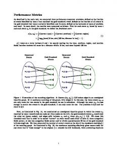
new approach eliminates the need for commercial software and custom data, while greatly reducing the level of effort needed to conduct these types of analyses. This allows a much broader base of stakeholders to conduct these analyses. The entire project described in this paper began from scratch and was completed, including documentation, in eight weeks. In this paper, free and open source software refers to software which may be legally used at no cost (free) and for which the source code is available (open source). Open data applies a similar concept to data sets, the data should be available for reuse by third parties with few or no restrictions, readily available at little or no cost, as well as discoverable (easy to find) and usable (coded using standard, open formats). There are a number of free to use tools that will provide routing and travel time information, however while these tools are available gratis (at no charge), they are not libre (with few or no restrictions). The terms of use restrictions on these tools and data sets restrict their use. Storage or the returned information for use in other types of analyses (as is required for accessibility analysis) is prohibited by their terms of use. The primary tool used for estimating transit accessibility for this analysis was OpenTripPlanner (14). OpenTripPlanner is a multi-modal trip planning software package intended to enable more transit agencies to provide door to door trip planning services over the web. It is free open source software released under the GNU Lesser General Public License. In our analysis, we used the tool to calculate the transit travel times between every traffic analysis zone (TAZ) in the area being studied (TAZ definition files are typically developed by a region’s MPO and can be obtained from the U.S. Census Bureau). OpenTripPlanner also requires a road network (for calculating walk distances) and transit schedules. The road network used was obtained from the OpenStreetMaps project (15). Other sources, including TIGER data could also be used, however OpenTripPlanner is already configured to use OpenStreetMaps data. Transit schedule data is also required. OpenTripPlanner makes use of schedules formatted to comply with the General Transit Feed Specification (GTFS) originally developed by Google (16). Although originally developed by Google as a standard format for transit agencies to feed data into Google’s proprietary trip planning service, dozens of transit agencies are now publishing their schedule information in this format as open data, with few or no restrictions on re-use. The availability of transit schedules in GTFS, combined with open software such as OpenTripPlanner is what made this project possible. While this combination of data and toolsets allows the calculation of transit travel times, there is no equivalent open data source for auto trip times. Therefore, in order to compare transit accessibility with auto accessibility an automotive router was developed as part of this project. This is described in more detail in the following sections. A graphical user interface tool was built that utilizes the calculated travel time matrix and the socio-economic data. This tool allows multiple types of visualizations, including travel time isochrones and cumulative opportunity and gravity model accessibility by TAZ, as well as the Modal Accessibility Gap. It also allows for browsing of the socio-economic data by TAZ. In addition, the tool can export KML files (17) that support 3D geographic visualization. Figure 1 shows an overview of the data inputs and major processes. Multiple internal data stores of shape, XML, and KML files are not shown.
McGurrin Greczner
1 2
3 4 5 6 7 8 9 10 11 12 13 14 15 16 17 18 19 20 21 22
6
FIGURE 1 Overall Process Flow
Development and Implementation The software developed to assess transportation accessibility requires TAZ data, including the TAZ boundary polygons in the ESRI Shapefile format, as well as socio-economic data for each TAZ. At a high level, the implementation sought to break down each TAZ to a singular point (centroid) from which to calculate accessibility. Using open source software as well as public data, travel times between each zone were calculated for both public transportation and automotive modes. Using census data along with the calculated trip times, various visualizations were also built to display the various metrics and models. The toolset included in QuantumGIS, an open source GIS tool, was used to calculate the geographic centroids for each of the zones from the given Shapefile. The centroids were then manually adjusted when necessary within a zone (e.g., when a zone included a large segment of parkland or water). This was adequate for our two proof-of-concept tests, which focused on heavily urbanized areas with small TAZs. We discuss below how the process can be modified for larger areas involving larger TAZs where a single centroid does not reasonably represent the entire TAZ. Shapefiles typically consist of multiple files and allow for data to be encoded, however they become cumbersome to manipulate programmatically because the data isn’t readily human-readable. In order to remedy this issue, the open source Shape2Earth plug-in for MapWindowGIS (another open source GIS tool) was used to convert both the TAZ and centroid Shapefiles into KML. The benefit to using KML is that it can then be displayed in tools such as Google Earth as well as Google Maps, and is much easier to work with via software.
McGurrin Greczner 1 2 3 4 5 6 7 8 9 10 11 12 13 14 15 16 17 18 19 20 21 22 23 24 25 26 27 28 29 30 31 32 33 34 35 36 37 38 39 40 41 42 43 44
7
Door to door travel times were calculated between every TAZ’s centroid. Within a region of 300 zones, 90,000 routes were computed for both transit and automotive trips. For purposes of the proof-ofconcept demonstration, the project focused on calculating sestination accessibilities for the morning commute to work. Therefore the trip planner was used to calculate the travel time for the goal of arriving at the desired destination by 9:00 am on a Wednesday. Of course, this could be expanded to couple travel to work with travel home, or to include a weighted average of various arrival times. For trips using public transportation, a maximum walking distance of 800 meters was imposed for the trip. For transit trips to and from the same zone a default value of 5 minutes was used. OpenTripPlanner was chosen as the means to calculate transit accessibility due to its comprehensiveness, robustness, and its on-going and active development. OpenTripPlanner is an open source multi-modal trip planning project implemented in Java. As a result, all other tools developed to calculate and visualize data were also written in Java. OpenTripPlanner uses OpenStreetMap data as well as General Transit Feed Specification files in order to build a graph network and calculate the subsequent fastest route between points. OpenStreetMap (OSM) files can be obtained either directly from their website, http://www.openstreetmap.org/export/, or for larger tracts of land, from http://downloads.cloudmade.com/. The latter site includes OSM files for all states as well as a number of countries. OSM files can be further altered using the command line tool, Osmosis, which has the ability to save a subsection of an OSM file, as well as the ability to merge multiple OSM files together. Configuration files for OpenTripPlanner were then used to build a network of roads and transit stops, using the specified OSM and GTFS files. Once completed, the graph can be loaded onto a local server and queried using the tools included in OpenTripPlanner. In order to suit the purposes of calculating the 100,000+ routes between TAZ’s within the District as well as the nearly 300,000 routes in the portion of King County that was modeled, OpenTripPlanner was amended to read in centroid data from a KML file, and in succession, query the graph for trip data to and from each of the respective TAZ’s. The response from OpenTripPlanner is returned in the form of an Itinerary. An Itinerary includes data describing everything from transfers to transit-specific information for each of the legs of the route. Itineraries were compiled for each TAZ, and once all routes were calculated for a zone, the results were outputted as XML to a specified directory. In the event that population, employment and housing data were specified within the configuration file, and were readily accessible in Excel format, such records were also included in the XML output. Unfortunately OpenTripPlanner does not provide adequate support for automotive routing. For demonstration purposes, in order to have estimates of auto travel accessibility, software was developed to parse TIGER/Line files provided by the census bureau. These files are, in general, not a good basis for route building and direction finding, however for purposes of our proof-of-concept, they were adequate for estimating urban travel times. Better network files can be substituted into the same approach. The developed software can currently handle one-way roads and turning restrictions can be easily added. Road Segments were extracted and stored in a local database which could then be queried to use Dijkstra’s algorithm (18) and calculate the fastest route between points. An interface was then designed to allow the user to configure the tool to load the TIGER database, specify a KML file describing the centroids, and finally input and output directories for the tool to use. The program creates a list of latitude and longitudinal points for each TAZ and then proceeds to the fastest route between every zone. In the event that a centroid did not fall on a road segment, the distance to the nearest segment was calculated and added to trip duration with the assumption that the car would have been able to get to that point at a rate of 15 miles per hour.
McGurrin Greczner 1 2 3 4 5 6 7 8 9 10 11 12 13 14 15 16 17 18 19
8
In order to estimate drive times, the Census Feature Class Code (CFCC) was used to determine an appropriate speed limit. This value was then scaled down slightly to account for possible traffic and congestion. Furthermore, routes received a turn penalty based on whether they had to turn right, left, or simply continue straight to the next leg of the trip. Turning left received the greatest penalty of a minute and a half, turning right was penalized by a minute, and going straight was penalized by a matter of seconds. Typically in a metropolitan setting during a morning commute, cars will inevitably run into stop lights and general congestion at intersections. In order to account for this, a nominal penalty for each intersection should be accounted for, despite the fact that a car will usually never have to stop at every intersection. Utilizing a turn penalty as well as a scaled down speed limit was determined to be the best way to efficiently generate realistic route times. After the drive times were collected for a particular TAZ, the associated XML output from the transit data was parsed and amended to include the drive time values. The information was then outputted to the specified directory. A standard XML data file format, defined by a RELAX NG schema (19) was used. Prior to developing a visualization for the collected data, both automotive and transit trip times were compared against online trip planners in order to check for accuracy. Transit data for a random sample of 215 routes was compared against the Washington Metropolitan Area Transit Authorities (WMATA) online trip planner. Figure 2 shows a comparison of the travel times calculated for the 215 routes:
OTP Calculated Trip Length (min)
120
OTP Trip Calculations vs WMATA Trip Calculations
100 80 60
Linear…
y = 0.9277x + 5.7447 R² = 0.8325
40 20 0 0
20 21 22 23 24 25 26 27 28 29
20
40 60 80 WMATA Calculated Trip Length (min)
100
120
FIGURE 2 A comparison of door to door travel time estimates using OpenTripPlanner and WMATA’s Trip Planner The strong correlation and significant agreement between the two tools provided confidence that OpenTripPlanner was indeed a valid source of trip data. Having perfect agreement was neither necessary nor expected, as different trip planners can make different assumptions on items such as estimated walk speed and the amount of buffer time to allow to ensure that connections are not missed. The linear approximation of the data has a Y-Intercept of around five minutes, and coupled with the slope, we would expect OpenTripPlanner to estimate travel times that are roughly five minutes faster on average then the
McGurrin Greczner
9
1 2 3 4 5 6 7 8 9 10 11 12
route predicted by WMATA. This result is in line with the hypothesis that WMATA is less aggressive in routing, ensuring more time is allowed in order to make connections. Over 83 percent of the variability in route times can be explained by the linearly approximated statistical model. Although the primary focus of this work was on transit accessibility, estimates of auto accessibility were also developed for purposes of comparison. Using a script, a sample of the automotive data and route times were compared against the driving directions tool provided by Google Maps. The nominal trip duration provided by Google was, on average, 31% faster then what had been calculated. However, a morning commute is often more likely to incur significant delay times, and the calculated drive times were considered to be reasonable for demonstration purposes, however more work is needed in this area. Google Maps driving directions, like those of other free direction providers, are not open data. The restrictions on use placed by the providers of these services prohibit them from being used as the direct source of travel times for the types of accessibility analysis described in this paper.
13 14 15 16 17 18 19 20 21 22 23 24 25 26 27 28 29 30 31 32
Sample Outputs Utilizing the results of the calculations, the GUI tool can display multiple types of maps, as well as export data in KML format for use in other 2D and 3D geographic displays. The calculated travel time matrices can be used to display isochrones maps, as shown in Figure 3. Figure 3 shows an isochrones map for transit trips in Washington, DC, for trips originating at the easternmost TAZ. The colors indicate destination zones reachable in 30 minutes or less, 30-45 minutes, 45-60 minutes, and greater than 60 minutes. The figure also shows how the data associated with the selected TAZ is displayed in the upper right of the user interface. Both transit and automotive accessibility can be displayed, using the results from either the cumulative opportunity model or the gravity model. Figure 4 shows a heat map of transit accessibility in the Seattle, Washington region calculated using the cumulative opportunity model. The GUI also allows for the model to be exported to KML, with the option to include with userspecified data-based extrusions. In these maps, the x and y axis are the geo-coordinates, the color can represent another variable, such as the Modal Accessibility Gap, while the Z access optionally displays either the same variable for emphasis or a different variable, such as number of households. This allows for complex mapping and the ability to explore connections between variables and models. The resulting KML data can be used for display in any tool that reads such data. Figure 5 is a display of the exported KML data using Google Earth, mapping the Modal Accessibility Gap index and households for Washington, DC.
McGurrin Greczner
1 2
10
Figure 3 Transit travel time isochrons for easternmost Traffic Analysis Zone
McGurrin Greczner
1 2
FIGURE 4 Transit accessibility in Seattle region using cumulative opportunity model
3 4
FIGURE 5 Modal Accessibility Gap (colors) versus households (height) for Washington, D.C.
11
McGurrin Greczner 1 2 3 4 5 6 7 8 9 10 11 12 13 14 15 16 17 18 19 20 21 22 23
24 25 26 27 28 29
30 31 32 33 34 35 36 37 38 39
12
Performance The runtime for a given region is dependent upon the following: Number of transit stops (GTFS file size) Sheer size of the area being calculated and how densely roads are packed near each other Number of TAZ’s or zones RAM available and processing power The number of routes which need be calculated increases exponentially with the number of Traffic Analysis Zones for a region. A large area with only a few zones can be computed just as quickly if not even quicker than a smaller region with more zones. On the other hand, memory is the core issue for the other three points. OSM files without alteration can be very large; King County for example requires 300 megabytes of space. Once parsed and built into a graph with the transit stop data, that number climbs even higher. In order for OpenTripPlanner to execute smoothly, at least four times that amount of memory needs to be allocated to the Java Virtual Machine. Failure to do so causes the program to stall while memory space is cleared from previous operations. Computation of larger regions without enough memory can cause a heap space exception to be fired which prevents further operation. Even with adequate RAM allocation, run times can be hindered by extensive road networks. As the number of edges in a network increases, the number of routes which must be assessed also increases. Automotive routes, however, are not as affected by these factors as are transit routes. Even for large metropolitan areas, routes are calculated fairly quickly and never run into memory issues. Run time estimates are shown in Table 1. The small city case represents approximately 300 TAZs and 100,000 vertices in the graph. The medium case represents approximately 400 TAZs and 300,000 vertices, while the large city represents approximately 500 TAZs and 500,000 vertices. Small City Medium City Large City Transit/Automotive Transit/Automotive Transit/Automotive 3 min/TAZ | 1 min/TAZ 9 min/TAZ | 4 min/TAZ 1 min/TAZ | 20 sec/TAZ TABLE 1 Run Times for Calculating the Travel Time Matrix As noted above, OpenTripPlanner produced reliable and accurate trip data to work with. The source code was easily altered to fit the needs of the project and provides a solid foundation from which to expand upon. At just over a year old, OpenTripPlanners' only downside is that it is still under development and naturally still contains the occasional bug, however it is undergoing active development.
Future Enhancements The proof-of-concept analyses looked only at the journey to work, with a targeted arrival time of 9 a.m. This analysis could be easily expanded to ensure that there is adequate access both to and from work destinations, or to examine access to retail or recreational opportunities. The proof-of-concept tests focused on two subsets of metropolitan planning areas. The use of these smaller regions simplified several factors. The TAZ’s for the two downtown regions are fairly small, so the concept of utilizing a single centroid point as the origin and destination for movement into and out of each zone was a reasonable simplification. Over wide areas, the zones become larger and transit service more sparse. In these cases, this simplification would introduce large errors. One approach for working with the larger zones and more diverse transit would be to utilize block level census
McGurrin Greczner
13
1 2 3 4 5 6 7 8 9 10 11 12 13 14 15 16 17 18 19 20 21 22 23 24 25 26
data. First, GIS tools would be used to calculate the catchment zones for each transit stop within a TAZ and then the subset of the population and jobs in the TAZ that have access to transit would be calculated and the final accessibility scores weighted accordingly. A similar approach is described in Polzin, et.al. (20). TAZ’s which totally lack transit options could be left out of the NxN matrix for computing travel times, reducing the required computation time. Similarly, for the relatively small test regions (319 zones for Washington, D.C. and 530 zones for Seattle) the geographic centroids for each zone were calculated using a GIS tool and then the locations were adjusted by hand for the subset of zones where this provided an unrealistic center for activity (e.g., when a large segment of the zone was water or parkland). A better alternative would be to utilize the block level census data to calculate one or more population or jobs weighted centroid location(s) for each zone. While a growing number of transit agencies are publishing their schedules in the GTFS format and freely allowing reuse, it is by no means universal. In the Washington, D.C. metropolitan region, the schedules for WMATA, the D.C. Circulator, and some other community bus services (e.g., Arlington County) are available. However schedules for other large systems, such as Fairfax County’s, are not yet published in GTFS. This was another reason our first proof-of-concept test was limited to the District of Columbia. While the availability of open transit data is growing rapidly, the same is not true for drive time information. While there are multiple free services for calculating directions including travel times, some with application programming interfaces (APIs), their terms of use do not permit archiving the results for reuse in other types of analysis, such as calculating accessibility. Vehicle probe data can provide travel times by time of day for both freeways and arterials, however today that data is collected by private companies and is proprietary. In today’s environment, the alternatives are to either implement a travel time estimator, as was done in this study, or to request the auto trip skim files used for transportation planning from the local metropolitan planning organization. In the future, new technologies such as IntelliDriveSM may provide an opportunity for a comprehensive open travel time data repository.
27 28 29 30 31 32 33 34 35 36 37 38 39
Conclusions There is an increasing push to move towards a more performance based approach for managing transportation systems. While not always feasible, it is desirable to measure the outcomes achieved (e.g., lives saved or access to jobs), rather than outputs (e.g., number of centerline miles with rumble strips or average speed on a road segment). Accessibility metrics are outcome focused. New free government data sets with liberal terms of use, combined with open software, are reducing the barriers to developing new applications in many fields, including transportation. In this paper, a new approach that utilizes these tools to calculate accessibility metrics has been described and demonstrated. While further work is needed, this proof of concept demonstrates that accessibility metrics can be utilized today by a broad group of prospective users, without major new investments in time or money. These metrics can provide technically sound, quantifiable measures that directly relate transportation with concepts such as “livability.” The utility of this approach will continue to grow as increasing amounts of transportation-related information is made available as open data.
McGurrin Greczner 1 2 3 4 5 6 7 8 9 10 11 12 13 14 15 16 17 18 19 20 21 22 23 24 25 26 27 28 29 30 31 32 33 34 35 36 37 38 39 40 41 42 43
14
References 1. Bipartisan Policy Center National Transportation Policy Project, Performance Driven: A New Vision for U.S. Transportation Policy, 2009. 2. Oberstar, J.L., J.L. Mica, J.L., P.A. DeFazio, J.J. Duncan, Jr. The Surface Transportation Authorization Act of 2009, A Blueprint for Investment and Reform, U.S. House of Representatives Committee on Transportation and Infrastructure, 2009 3. Paniati, J.L. U.S. Department of Transportation Perspective on Federal Reauthorization. Presented at 89th Annual Meeting of the Transportation Research Board, Washington, D.C., 2010. 4. HUD-DOT-EPA Interagency Partnership for Sustainable Communities. U.S. Environmental Protection Agency, www.epa.gov/smartgrowth/partnership/index.html#livabilityprinciples. Accessed July 8, 2010. 5. Handy, S. Accessibility- vs. Mobility-Enhancing Strategies for Addressing Automobile Dependence in the U.S., Prepared for the European Conference of Ministers of Transport, www.des.ucdavis.edu/faculty/handy/ECMT_report.pdf, 2002. Accessed July 12, 2010. 6. Litman, T. Evaluating Accessibility for Transportation Planning, Victoria Transport Policy Institute, 2010. 7. Litman, T. Accessibility: Evaluating People’s To Reach Desired Goods, Services and Activities, from The Online TDM Encyclopedia, Victoria Transport Policy Institute, www.vtpi.org/tdm/tdm84.htm, 2010. Accessed July 12, 2010. 8. Pratt, R.H. and T. J. Lomax. Performance Measures for Multimodal Transportation Systems, in Transportation Research Record 1518, TRB, National Research Council, Washington, D.C. 1996. 9. Rodrigue, J., C. Comtois, B. Slack. The Geography of Transport Systems, Routledge, New York, 2009. 10. Handy, S.L. and D.A. Neimeier, Measuring Accessibility: An Exploration of Issues and Alternatives in Environment and Planning A, 29(7), 1997. 11. El-Geneidy, A.M. and D.M. Levinson, Access to Destinations: Development of Accessibility Measures, Report Number MN/RC-2006-16. Minnesota Department of Transportation, St. Paul, Minnesota, 2006. 12. Kwok R.C.W. and A.G.O. Yeh. The Use of Modal Accessibility Gap as an Indicator for Sustainable Transport Development in Environment and Planning A 36(5) 921 – 936, 2004. 13. Grengs, J. Measuring change in Small-Scale Transit Accessibility with Geographic Information Systems, Transportation Research Record 1887, TRB, National Research Council, Washington, D.C. 2004. 14. OpenPlans, OpenTripPlanner Developer Site, www.openplanner.org. Accessed July 26, 2010. 15. OpenStreetMap, OpenStreetMap Wiki Main, wiki.openstreetmap.org/wiki/Main_Page. Accessed July 26, 2010. 16. Google, General Transit Feed Specification, code.google.com/transit/spec/transit_feed_specification.html, 2010. Accessed July 26, 2010. 17. Google, KML Documentation Introduction, code.google.com/apis/kml/documentation/, Accessed July 27, 2010. 18. Dijkstra, E. W. A Note on Two Problems in Connexion with Graphs, in Numerische Mathematik 1, 1959.
McGurrin Greczner 1 2 3 4 5
15
19. Oasis, Relax NG Specification, www.relaxng.org/spec-20011203.html, 2001. Accessed July 26, 2010. 20. Polzin, S. E., R. M. Pendyala, S. Navari. Development of Time-of-Day-Based Transit Accessibility Analysis Tool, In Transportation Research Record 1799, TRB, National Research Council, Washington, D.C., 2002.