[2] B. A. Allan, R. C. Armstrong, A. P. Wolfe, J. Ray, D. E. Bernholdt, and J. A. Kohl, âThe ... [3] S. Lefantzi, J. Ray, and H. N. Najm, âUsing the Common Component.
Performance Modeling of Component Assemblies with TAU N. Trebon† , A. Morris† , J. Ray∗ , S. Shende† and A. Malony† ∗ Sandia
National Laboratories, Livermore, CA 94551 {jairay}@ca.sandia.gov and † University of Oregon, Eugene, OR 97403 {ntrebon,amorris,sameer,malony}@cs.uoregon.edu
I. I NTRODUCTION The Common Component Architecture (CCA) is a component-based methodology for developing scientific simulation codes. This architecture consists of a framework which enables components, (embodiments of numerical algorithms and physical models) to work together. Components publish their interfaces and use interfaces published by others. Components publishing the same interface and with the same functionality (but perhaps implemented via a different algorithm or data structure) may be transparently substituted for each other in a code or a component assembly. Components are compiled into shared libraries and are loaded in, instantiated and composed into a useful code at runtime. Details regarding CCA can be found in [1], [2]. An analysis of the process of decomposing a legacy simulation code and re-synthesizing it as components can be found in [3], [4]. Actual scientific results obtained from this toolkit can be found in [5], [6]. Components exist so that they can be reused. Thus, the component writer is rarely the sole user of the components. A component writer can be expected to ensure the correctness of the component. The performance, however, is of primary importance to the component user who may not be familiar with the implementation to the component. Thus, in the context of HPC (high performance computing) with components, one needs a reliable way of measuring the performance of each implementation of a component nonintrusively and correlate the performance with the problem size to create a performance model. This was addressed in [7], where a prototypical performance measurement and modeling infrastructure (a set of performance related components based on the TAU performance system [8], [9] for monitoring and recording performance metrics of a scientific simulation) was demonstrated. In this paper we present how these performance models, may be used to obtain an approximately optimal component assembly i.e., an optimal code. Once a performance model has been created for each of the components and their implementations, it is possible to construct a global performance model for the application. By comparing global performance models utilizing different subsets (implementations) of components, it is possible to select an optimal set of component implementations for a given prob-
lem. However, simply selecting the optimal implementation of each component does not guarantee an optimal global solution because the individual performance models do not consider the interactions between components (e.g., cost of translating one data structure to another if the interacting components have different data layouts). If the number of components and their implementations are small, one may adopt the bruteforce approach of enumerating all the possible realizations of the component assembly, constructing and evaluating their global performance models, and choosing the optimal one. However, typical scientific codes consist of assemblies of 10 to 20 components. If each component has three implementations, the solution space consists of 310 to 320 possible realizations, which makes the brute-force approach of comparing each realization unfeasible. We propose a simple rule-based approach to reduce the solution space by eliminating “insignificant” components. A component is insignificant if it does not significantly contribute to the overall performance of the application. These components are eliminated from the global performance model, leaving behind the “dominant” sub-assemblies, or cores. Once the cores have been selected, an optimal assembly can be realized through comparing the reduced number of global performance models from these cores. The optimal component assembly (consisting entirely of the cores) may then be extended into a functioning component assembly by using (adding) any implementation of the “insignificant” components. This ensures that the final assembly will be close to optimal. Runtime automated optimization of codes, as done by Autopilot [10], [11] and Active Harmony [12] are closest to our approach as outlined here and in [7]. Both require the application to identify performance parameters (and the valid values that they can take) to a tuning infrastructure. This infrastructure also monitors their performance, which in case of Active Harmony is provided by a function (the objective function) implemented by the application itself. Each of the parameters are perturbed and the application run to obtain the effect of the perturbation. Active Harmony relies upon a simplex algorithm to identify the optimal values of the parameters while Autopilot uses fuzzy logic. Both (Active Harmony and Autopilot) require the identification of “bad” regions in parameter space, so that the optimization search
may be concluded faster by avoiding these regions. Active Harmony also has an infrastructure to swap in/out multiple libraries in order to identify an optimal implementation. Neither of these approaches are quite right for us. We can afford many evaluations of the objective function since it is an algebraic formula synthesized out of multiple component performance models. However, no approach will stand up to exponential complexity. Our strategy has been to identify the core set of parameters (component implementations) that significantly affect performance and to perform a brute-force evaluation/optimization only on the core. II. P ERFORMANCE M EASUREMENT The infrastructure used to measure performance in HPC environment is described in [7]. The framework consists of three component types. First, lightweight proxies are interposed between the caller and the callee components and trap any method calls, enabling performance measurements to be taken. The second component type is responsible for making the performance measurements, including timer creation and hardware interaction. The measurement system makes use of the TAU measurement library [8] via a TAU component. The final component type is the Mastermind, which is responsible for gathering, storing, and reporting the measurement data. Each proxy is connected to the Mastermind component, which provides functionality to turn measurements on and off. The Mastermind, in turn, is connected to TAU, which provides the functionality to create and manage timers, as well as access hardware counters. Because of the proxies’ lightweight nature, the creation is a mechanical process. We have developed a tool that automatically generates a proxy for a given component This tool is based on the Program Database Toolkit [13], which allows for analysis and processing of C++ source code. A Proxy is create for a single port. For a component that provides multiple ports, multiple proxies can be generated. A similar tool was created to automatically generate the Mastermind component. As a result of these tools, a measurement framework can be easily created for a CCA application. III. A N A PPROXIMATE A PPROACH Table I displays the average results from the four processor run of the hydro-shock simulation (as described in [7]) averaged over the four CPUs. The exclusive time represents the time spent in the given routine, minus the time spent in all instrumented routines that occur prior to the routine’s completion. Inclusive time measures the time spent from the start of the routine until routine completion. As one can see, the ErrorEstimator (ee proxy) component’s routine alone contributes over 30 seconds, or approximately 33% of the total execution time, while the BoundaryConditions (bc proxy) component contributes a mere 38 milliseconds, or less than 1%. Our aim is to propose an algorithm that identifies these insignificant components and removes them from consideration during the optimization process. To accomplish this, we
TABLE I T HE TABLE
DISPLAYS THE EXCLUSIVE
TIMES ( DEFINED IN
(E XCL .) AND INCLUSIVE (I NCL .)
S ECTION III, AS WELL AS THE
INCLUSIVE
PERCENTAGE FOR EACH OF THE INSTRUMENTED ROUTINES OF A GIVEN COMPONENT.
Component Name driver proxy rk2 proxy ee proxy flux proxy sc proxy efm proxy grace proxy icc proxy grace proxy icc proxy stats proxy c proxy rk2 proxy cq proxy bc proxy
A LL TIMES ARE
Method name go() Advance() Regrid() compute() compute() compute() GC Synch() prolong() GC regrid above() restrict() compute() compute() GetStableTimestep() compute() compute()
IN MILLISECONDS .
Excl. time 285 6,887 31,607 3,118 11,131 7,549 1,956 1,044 644 815 212 129 5 86 38
Incl. Time 90,785 34,411 32,582 22,156 11,131 7,549 3,689 1,044 946 815 271 253 157 150 38
% 96 36.4 34.5 23.4 11.8 8.0 3.9 1.1 1.0 0.9 0.3 0.3 0.2 0.2 0.0
extend our “proxying” technique described in [7] to construtct a call-graph as the component application executes. Upon termination, the call-graph is written to a file. A pruning application then reconstructs the call-graph from the file and performs the pruning algorithm. Figure 1 shows the entire call graph for the simulation that we analyze (see [7] for details). Since a component may be invoked from multiple places i.e., it may exist on many call paths, it may appear as multiple nodes on that graph. Once this graph is created, it can be traversed, and based upon a set of rules, branches classified as insignificant can be pruned off. “Insignificance”, in our case is decided based on the inclusive time of a component. The resulting graph will be an optimized core tree, that identifies the major contributors to the code assembly’s global performance. The selection of the optimal solution can then be based upon the performance of these dominant core components. Any combination of pruned component instances can then be included to complete an approximately optimal global solution. A. Algorithm In the following, let CJ represent the set of children of node J. Let Ti , i ∈ CJ be the inclusive time of child i of node J. Let J have NJ children, i.e., the order of the finite set CJ is NJ . When examining the children of a given node, we see that two cases arise : 1) The total inclusive time of the children is insignificant compared to the inclusive time of node J i.e., X Ti /TJ < α, i,i∈CJ
where 0 < α � 1. Thus the children contribute little to the parent node’s performance and may be safely eliminated from further analysis. α is typically around 0.1 i.e., 10%.
Fig. 1. The component call-graph for the shock hydro simulation. Along with the component instance name, the inclusive time, in microseconds, is included in each node.
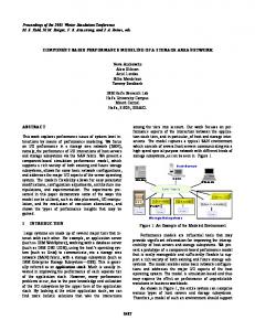
Fig. 2. A simple call-graph example with pruned branches colored red and node shaded.
2) The total inclusive time of the children is a substantial fraction of node J’s inclusive P time i.e., the children contribute significantly and i,i∈CJ Ti /TJ > α. In this case the children are analyzed to identify if dominant siblings exist. Let X T¯ = Ti /NJ i,i∈CJ
be the average or “representative” inclusive time for the elements of CJ . We then iterate through each node i, i ∈ CJ , eliminating the elements of CJ where Ti /T¯ < β. Thus, children of J whose contributions are small relative to a representative figure are eliminated. Typically, β is chosen to be around 0.1 i.e. 10%. IV. E XAMPLES In order to test our approach, it was first applied to a series of simple call-graphs in order to ensure its correctness. One of these examples is described in Section IV-A. The pruning algorithm was then applied to a call-graph that was created from an actual scientific simulation. Results are presented in Sections IV-B and IV-C.
Fig. 3. The resulting call-graph after pruning using levels of 10% for both thresholds i.e., α = β = 0.1
B. Example 2: Shock-Hydro with 10% thresholds Our pruning approach was then applied to a real scientific simulation code. The complete component call-graph is depicted in Figure 1. Each node in the graph contains the name and the inclusive count for the given node. Using the default threshold values of 10%, the original call-graph of 19 nodes (12 unique component instances) is reduced to a callgraph of 8 nodes (8 unique component instances). The amount of unique component instances has been reduced by roughly 33%. These results are depicted in Figure 3.
A. Example 1: Dominant Path
C. Example 3: Shock-Hydro with variable thresholds
Figure 2 depicts a simple call-graph that consists of only six nodes. The algorithm works in a depth-first search. Starting at the root, the two children, B and C, together do significantly contribute to the parent’s inclusive execution time, and so each branch is preserved and searched. First, the branch leading to node B is examined, and since it contributes significantly, it remains as part of a dominant path. At this point, node B’s children are examined to see if they are significant to node B; they are not and so nodes D and E are both immediately pruned. Next, node C is examined to see if it is significant to its parent, node A. Node C is determined to be insignificant is removed. In the figures hereafter, we will follow the convention of shading pruned branches.
Our pruning approach was also applied with threshold levels set to 5% and 20%. These results are shown in Figures 4, and 5 respectively. In the case of the 5% threshold levels, one component instance (ICC) is kept, rather than removed, compared with the 10% thresholds. Similar results are observed when comparing the 10% and 20% graphs. As expected, with a higher threshold, we pruned off a branch that the lower thresholds identified as significant. Also, with the 20% thresholds only 7 out of the 12 components were preserved in the component assembly. Thus this method trades speed (achieving a small “core” call-graph) against accuracy (recovering the actual inclusive time of the call-graph root from the “core” call-graph) but allows one to conduct a
Fig. 4. The resulting call-graph after pruning using levels of 5% for both thresholds, i.e., α = β = 0.05.
Fig. 5. The resulting call-graph after pruning using levels of 20% for both thresholds, i.e., α = β = 0.20.
sensitivity (with respect to α and β) analysis if it is deemed important. V. C ONCLUSIONS In this paper we have presented a simple algorithm to identify the dominant components (from a performance point of view) in a component assembly. This algorithm was tested on a call-graph created by monitoring a hydrodynamics simulation as analyzed in [7]. The inclusive execution times, though obtained from actual measurements, could have also been obtained from performance models. Starting with a call-graph of 19 nodes (12 separate components), with thresholds (α, β) of 10 % we were able to determine a core component assembly of 8 nodes. The resulting call-graph represents a smaller solution space to search for the optimal set of component instances to solve a given problem. This algorithm successfully reduced the call-graph of a real scientific simulation by roughly 41 % and the number of realizations of component assemblies from 312 to 37 (assuming that 3 implementations of each component exist), a saving of over two orders of magnitude when the thresholds were set to 20%. In the future we will address the construction of the composite performance model for the entire component assembly from the call-graph. The current monitoring infrastructure is being extended to record the traversals of the branches of the
call-graph along with the problem size that the components are presented with per invocation. For static scientific problems (e.g. PDEs solved on a static mesh) the problem size is expected to remain constant for the duration of the simulation. This constraint is violated for dynamic approaches where the algorithm adapts to the problem (e.g. PDEs solved on an adaptively refined mesh) and the problem size per component invocation is expected to change during the course of the simulation. In such a case, the deterministic component performance models will be embedded in a stochastic framework to provide the “most probable” performance of a component assembly as well as some (mathematically rigorous) measure of the uncertainty associated with the “most probable” number. R EFERENCES [1] R. Armstrong, D. Gannon, A. Geist, K. Keahy, S. Kohn, L. McInnes, S. Parker, and B. Smolenski, “Towards a Common Component Architecture for High Performance Scientific Computing.” in Proceedings of the 8th International Symposium on High Performance Distributed Computing, 1999. [2] B. A. Allan, R. C. Armstrong, A. P. Wolfe, J. Ray, D. E. Bernholdt, and J. A. Kohl, “The CCA Core Specifications in a Distributed Memory SPMD Framework,” Concurrency: Practice and Experience, vol. 14, pp. 323–345, 2002, also at http://www.cca-forum.org/ccafe03a/index.html. [3] S. Lefantzi, J. Ray, and H. N. Najm, “Using the Common Component Architecture to Design High Performance Scientific Simulation Codes,” in Proceedings of the International Parallel and Distributed Processing Symposium, Nice, France, April 2003. [4] S. Lefantzi and J. Ray, “A Component-based Scientific Toolkit for Reacting Flows,” in Proceedings of the Second MIT Conference on Computational Fluid and Solid Mechanics. Boston, Mass.: Elsevier Science, 2003. [5] J. Ray, C. Kennedy, S. Lefantzi, and H. N. Najm, “High-order Spatial Discretizations and Extended Stability Methods for Reacting Flows on Structured Adaptively Refined Meshes,” in Third Joint Meeting of the U.S. Sections of The Combustion Institute, Chicago, Illinois, March 2003, distributed on a CD. [6] S. Lefantzi, C. Kennedy, J. Ray, and H. N. Najm, “A Study of the Effect of Higher Order Spatial Discretizations in SAMR (Structured Adaptive Mesh Refinement) Simulations,” in Proceedings of the Fall Meeting of the Western States Section of the The Combustion Institute, Los Angeles, California, October 2003, distributed on a CD. [7] J. Ray, N. Trebon, S. Shende, R. C. Armstrong, and A. Malony, “Performance Measurement and Modeling of Component Applications in a High Performance Computing Environment : A Case Study,” Sandia National Laboratories, Tech. Rep. SAND2003-8631, June 2003, Also submitted to International Parallel and Distributed Computing Symposium, 2004. [8] “TAU: Tuning and Analysis Utilities,” http://www.cs.uoregon.edu/research/paracomp/tau/. [9] A. D. Malony and S. Shende, Distributed and Parallel Systems: From Concepts to Applications. Norwell, MA: Kluwer, 2000, ch. Performance Technology for Complex Parallel and Distributed Sys tems, pp. 37–46. [10] R. L. Ribler, H. Simitci, and D. A. Reed, “The Autopilot PerformanceDirected Adaptive Control System,” Performance Data Mining, vol. 18, pp. 175–187, 2001, Special Issue : Future Generation Computer Systems. [11] R. L. Ribler et al, “Autopilot : Adaptive Control of Distributed Applications,” in Proceedings of the 5 th IEEE International Symposium on High Performance Distributed Computing, 1998, Chicago, IL, USA. [12] I.-H. C. Cristian Tapus and J. K. Hollingsworth, “Active Harmony : Towards Automated Performance Tuning,” in Proceedings of the 2002 ACM/IEEE Conference on Supercomputing, 2002. [13] “PDT: Program Database Toolkit,” http://www.cs.uoregon.edu/research/paracomp/pdtoolkit/.