Performance of Decomposition-Based Many-Objective ... - IEEE Xplore

This article has been accepted for publication in a future issue of this journal, but has not been fully edited. Content may change prior to final publication. Citation information: DOI 10.1109/TEVC.2016.2587749, IEEE Transactions on Evolutionary Computation

Performance of Decomposition-Based Many-Objective Algorithms Strongly Depends on Pareto Front Shapes Hisao Ishibuchi, Yu Setoguchi, Hiroyuki Masuda, and Yusuke Nojima Abstract—Recently a number of high performance manyobjective evolutionary algorithms with systematically generated weight vectors have been proposed in the literature. Those algorithms often show surprisingly good performance on widely used DTLZ and WFG test problems. The performance of those algorithms has continued to be improved. The aim of this paper is to show our concern that such a performance improvement race may lead to the overspecialization of developed algorithms for the frequently used many-objective test problems. In this paper, we first explain the DTLZ and WFG test problems. Next we explain many-objective evolutionary algorithms characterized by the use of systematically generated weight vectors. Then we discuss the relation between the features of the test problems and the search mechanisms of weight vector-based algorithms such as MOEA/D, NSGA-III, MOEA/DD and  -DEA. Through computational experiments, we demonstrate that a slight change in the problem formulations of DTLZ and WFG deteriorates the performance of those algorithms. After explaining the reason for the performance deterioration, we discuss the necessity of more general test problems and more flexible algorithms. Keywords—Many-objective optimization, many-objective test problems, many-objective evolutionary algorithms, decompositionbased evolutionary algorithms.

f2 1.0 0.8 0.6 0.4 0.2 0.0 0.0

0.2

0.4

0.6

0.8

1.0

f1

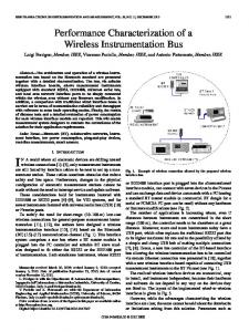
Fig. 1. Randomly generated 200 solutions and the Pareto front of a test problem in Fonseca & Fleming [2].

f2 6 5 4

I. INTRODUCTION

3

Recently the development of evolutionary multi-objective optimization (EMO) algorithms was discussed from the point of view of co-evolution with test problems in [1] where the Pareto front was compared with randomly generated initial solutions to explain the characteristic features of each test problem. For example, Fig. 1 shows a test problem in [2] used for performance evaluations of EMO algorithms in the mid1990s. As we can see from Fig. 1, some initial solutions are very close to the Pareto front. This observation may explain why non-elitist EMO algorithms such as NSGA [3] and NPGA [4] with no strong convergence property were proposed in the mid-1990s. However, initial solutions of a test problem in Fig. 2 [5] are not close to the Pareto front. Thus we need strong convergence whereas no strong diversification is needed in Fig. 2 (since randomly generated initial solutions have a large diversity). These observations explain why elitist EMO algorithms such as SPEA [6], NSGA-II [7] and SPEA2 [8] were proposed around 2000. In these algorithms, Pareto dominance was used as the main fitness evaluation criterion together with a secondary criterion for diversity maintenance.

2

Manuscript received December 17, 2015. This work was partially supported by KAKENHI Grant Numbers 24300090, 26540128 and 16H02877. H. Ishibuchi, Y. Setoguchi, H. Masuda and Y. Nojima are with Department of Computer Science and Intelligent Systems, Osaka Prefecture University, Japan (e-mail: [email protected], [email protected], [email protected], [email protected])

Pareto Front

Pareto Front

1 0 0.0

0.2

0.4

0.6

0.8

1.0 f1

Fig. 2. Randomly generated 200 solutions and the Pareto front of a twoobjective ZDT1 problem [5].

In parallel with the increase in the popularity of the Pareto dominance-based EMO algorithms [6]-[8], many-objective test problems called DTLZ [9] and WFG [10] were proposed as scalable test problems where the number of objectives can be arbitrarily specified. Multi-objective knapsack problems [6] were also generalized to many-objective test problems with up to 25 objectives [11], [12]. The DTLZ, WFG and knapsack problems were repeatedly used for demonstrating difficulties of many-objective optimization for the Pareto dominance-based EMO algorithms [13]-[16]. When an EMO algorithm is applied to a many-objective problem, almost all solutions in a population become non-dominated with each other in very early generations (e.g., within ten generations) before they converge to the Pareto front. This means that the Pareto dominance-based selection pressure toward the Pareto front becomes very weak. As a result, convergence ability of Pareto dominance-based EMO algorithms is severely degraded by the increase in the number of objectives.

1089-778X (c) 2016 IEEE. Translations and content mining are permitted for academic research only. Personal use is also permitted, but republication/redistribution requires IEEE permission. See http://www.ieee.org/publications_standards/publications/rights/index.html for more information.


MOEA/D [25] searches for well-distributed solutions using systematically generated weight vectors. As an example, we show a set of 91 weight vectors for a three-objective problem in Fig. 3. In Fig. 4, we show an example of obtained solutions by MOEA/D-PBI with  = 5 [25] for a three-objective DTLZ2 problem [9]. Well-distributed solutions were obtained in Fig. 4 using the uniformly distributed weight vectors in Fig. 3. In Fig. 3 and Fig. 4, a one-to-one mapping was realized between the weight vectors in Fig. 3 and the obtained solutions in Fig. 4. However, this is not always the case. As examined in [33], the number of obtained non-dominated solutions by MOEA/D is often much smaller than the number of weight vectors. This is because (i) a single good solution can be shared by multiple weight vectors and (ii) all solutions are not always non-dominated. Recently proposed many-objective algorithms [27]-[32] with the MOEA/D framework have mechanisms for improving both the convergence of solutions toward the Pareto front and their uniformity over the entire Pareto front. Their common feature is the use of systematically generated weight vectors. In those algorithms, reference points and/or reference lines are constructed using the weight vectors. Surprisingly good results were reported by those weight vector-based algorithms on the DTLZ and WFG problems in the literature. For example, the average inverted generational distance (IGD) over 20 runs on a 15-objective DTLZ2 problem was reported in [29] as 1.726  102 by NSGA-III, 1.133  102 by  -DEA, and 6.005  103 by MOEA/D-PBI. In Fig. 5, we show the reference points used for the IGD calculation in [29] and a set of obtained solutions by a single run of MOEA/D-PBI with  = 5 (IGD is 5.590  103 in Fig. 5). The obtained solution set in Fig. 5 (b) is almost the same as the reference point set in Fig. 5 (a).

1.0 w3 0.5 0.0 0.0

w3 0.5

0.5

w2 0.0 0.0 w1

0.5

1.0

0.5

0.0

1.0

1.0

0.5

0.0 w1

1.0 w2

Fig. 3. Example of weight vectors used in MOEA/D (91 weight vectors).

1.0

1.0 f3 0.5 0.0 0.0

f3 0.5

f2 0.0 0.0 f1

0.5

1.0

0.0

0.5

0.5

1.0

1.0

0.5

0.0 f1

1.0 f2

Fig. 4. Example of obtained non-dominated solutions by MOEA/D-PBI for a three-objective DTLZ2 problem using the 91 weight vectors in Fig. 3. 1.0 Objective Value

Whereas MOEA/D [25] was not originally proposed for many-objective problems, its high performance as a manyobjective optimizer was observed in the literature (e.g., [16], [26]). Recently, a number of new many-objective algorithms have been proposed using the framework of MOEA/D (e.g., IDBEA [27], MOEA/D-DU [28], EFR-RR [28] and  -DEA [29]). Some other algorithms (e.g., NSGA-III [30], MOEA/DD [31] and U-NSGA-III [32]) can be viewed as using hybrid mechanisms of the Pareto dominance-based fitness evaluation and the MOEA/D framework

1.0

0.8 0.6 0.4 0.2 0.0

1

2

3

4

5

6 7 8 9 10 11 12 13 14 15 Objective Number

(a) Reference points. 1.0 Objective Value

For improving the convergence ability for many-objective problems, various approaches have been proposed such as the modification of the Pareto dominance relation [17] and the introduction of an additional ranking mechanism [18]-[21]. The use of a different fitness evaluation mechanism was also actively studied. Approaches in this direction can be classified into two categories. One is an indicator-based approach such as SMS-EMOA [22] and HypE [23]. The advantage of EMO algorithms in this category is a sound theoretical support, which is based on a direct relation between many-objective optimization and indicator optimization. Their main difficulty is heavy computation load for fitness evaluation. The other category is characterized by the use of a scalarizing function for fitness evaluation such as MSOPS [24] and MOEA/D [25]. These algorithms are referred to as decomposition-based or scalarizing function-based algorithms.

0.8 0.6 0.4 0.2 0.0

1

2

3

4

5

6 7 8 9 10 11 12 13 14 15 Objective Number

(b) Obtained solutions by a single run of MOEA/D-PBI. Fig. 5. Reference points for the IGD calculation and a set of obtained solutions by MOEA/D-PBI with  = 5 for a 15-objective DTLZ2 problem.

Whereas difficulties of many-objective problems were repeatedly pointed out in the literature (e.g., see survey papers [12], [34], [35]), Fig. 5 and the reported results in [27]-[32] may suggest that some DTLZ and WFG problems are not difficult. In this paper, we first examine why surprisingly good results were obtained for some DTLZ and WFG test problems.



Then we show that a slight change in the DTLZ and WFG formulations degrades the performance of weight vector-based many-objective algorithms. Our experimental results suggest the overspecialization of those algorithms for the test problems. This paper is organized as follows. In Section II, we briefly explain the DTLZ [9] and WFG [10] problems. We focus on the shape of the Pareto front of each test problem. In Section III, we explain a common search mechanism of weight vectorbased algorithms such as MOEA/D-PBI [25],  -DEA [29] and NSGA-III [30]. We also discuss the relation between the shape of the Pareto front of each test problem and the common search mechanism of those algorithms. In Section IV, we demonstrate their high performance on the DTLZ and WFG problems. We also demonstrate severe performance deterioration by a slight change in the problem formulations of DTLZ and WFG: All objectives are multiplied by (1). In Section V, we explain why the performance of the weight vector-based algorithms is sensitive to such a slight change. We also discuss the necessity of more general test problems and more flexible algorithms. Finally we conclude this paper in Section VI. II. MANY-OBJECTIVE TEST PROBLEMS In general, an M-objective minimization problem with a decision vector x and its feasible region X is written as Minimize f1 ( x ) , f 2 ( x ) , ..., f M ( x ) subject to x  X , (1) where f i ( x ) is the ith objective to be minimized (i = 1, 2, ..., M). In the EMO community, multi-objective problems with four or more objectives (i.e., M  4 ) are often referred to as many-objective problems [12], [34], [35]. Scalable many-objective test problems called DTLZ [9] and WFG [10] have been frequently used to evaluate manyobjective algorithms in the literature. Table I summarizes many-objective test problems used for performance evaluation of recently proposed weight vector-based algorithms [27]-[32]. For comparison, we also show multi-objective test problems used for evaluating MOEA/D in [25]. We can see from this table that DTLZ1-4 and WFG1-9 have often been used in the literature. In this section, we briefly explain those test problems. A. DTLZ Test Problems The DTLZ test suite was designed by Deb et al. [9] as a set of nine scalable test problems (DTLZ1-9). The number of decision variables (say n) of M-objective DTLZ1-7 problems is specified as n = M + k  1 where k is a parameter. The value of k is often specified as k = 5 in DTLZ1, k = 10 in DTLZ2-6, and k = 20 in DTLZ7. In DTLZ8-9, the number of decision variables is specified as n = 10M. Let y*= (y*1 , y*2 , ..., y*M ) be a Pareto optimal solution in the M-dimensional objective space of each test problem. The Pareto front of each of the first four test problems (DTLZ1-4) can be represented by the following formulations [9]: M

DTLZ1:  yi*  0.5 and yi*  0 for i = 1, 2, …, M. i 1

M

Ref.

Publication Year

Proposed Algorithm

[25]

2007

MOEA/D

[27]

2015

I-DBEA

[28]

2016

MOEA/D-DU EFR-RR

[29]

2016

 -DEA

[30]

2014

NSGA-III

[31]

2015

MOEA/DD

[32]

2016

U-NSGA-III

Test Problems

Number of Objectives

Knapsack ZDT1-4, 6 DTLZ1-2 DTLZ1-4 DTLZ5(I, M) WFG1-9 DTLZ1-4, 7 WFG1-9 S-DTLZ1-2 DTLZ1-4, 7 S-DTLZ1-2 WFG1-9 DTLZ1-4 WFG6-7 S-DTLZ1-2 DTLZ1-4 WFG1-9 ZDT1-4, 6 DTLZ1-2 S-DTLZ1-2

2, 3, 4 2 3 3, 5, 8, 10, 15 3, 5, 8, 10, 15 3, 5, 10, 15 2, 5, 8, 10, 13 2, 5, 8, 10, 13 2, 5, 8, 10, 13 3, 5, 8, 10, 15 3, 5, 8, 10, 15 3, 5, 8, 10, 15 3, 5, 8, 10, 15 3, 5, 8, 10, 15 3, 5, 8, 10, 15 3, 5, 8, 10, 15 3, 5, 8, 10 2 3, 5 ,8, 10 3, 5, 8, 10

As shown in Table I, DTLZ1-4 have been frequently used for performance evaluation of many-objective algorithms. This is because their Pareto fronts are represented by the simple formulations in (2) and (3). DTLZ5-6 were originally proposed as many-objective test problems with degenerate Pareto fronts in [9]. However, their Pareto fronts are not degenerate when they have four or more objectives ([10], [36], [37]). Constraint conditions were introduced to remove the non-degenerate parts of the Pareto fronts [36], [37]. The Pareto fronts of DTLZ7-9 cannot be represented by a simple form as in (2) or (3).

B. WFG Test Problems The WFG test suite was proposed by Huband et al. [10] as a set of nine scalable test problems (WFG1-9). An M-objective WFG problem has k position-related variables and l distancerelated variables. Thus the total number of decision variables is n = k + l. The suggested values of k and l in [10] were k = 4 and l = 20 for two-objective problems and k = 2(M  1) and l = 20 for problems with more than two objectives. However, different specifications have been used in the literature. For example, they were specified as k = M  1 and l = 24  (M  1) in [29]. These specifications [29] are used in this paper. Since l should be an even number in WFG2 and WFG3, the specification of l is slightly changed as l = 16 for M = 8 and l = 14 for M = 10 only in WFG2 and WFG3 in this paper. WFG1 has a complicated Pareto front, which cannot be represented by a simple form as in (2) or (3). The Pareto front of WFG2 is disconnected. WFG3 was originally designed as a many-objective test problem with a degenerate Pareto front. However, its Pareto front is not degenerate when it has three or more objectives as recently pointed out in [38]. All the other test problems (i.e., WFG4-9) have the following Pareto front: 2

(2)

DTLZ2-4:  ( yi* ) 2  1 and yi*  0 for i = 1, 2, …, M. (3) i 1

Table I. Many-objective test problems used in each study on weight vector-based many-objective evolutionary algorithms.

M  y*  WFG4-9:   i   1 and yi*  0 for i = 1, 2, …, M. (4) i 1  2i 

One important feature of the Pareto fronts of WFG4-9 in (4) is that the domain of each objective has a different



magnitude (e.g., 0  y1*  2 and 0  y10*  20 ). This explains why most of the recently proposed many-objective algorithms [27]-[30], [32] in Table I have normalization mechanisms of the objective space. Since MOEA/D [25] has no normalization mechanism, good results have not been reported for manyobjective WFG problems in the literature. C. Common Feature of DTLZ1-4 and WFG4-9 By normalizing the range of the Pareto front for each objective into the unit interval [0, 1], the Pareto fronts of DTLZ1-4 and WFG4-9 can be rewritten as follows: M

DTLZ1:  yi*  1 and yi*  0 for i = 1, 2, …, M. i 1

(5)

DTLZ2-4 and WFG4-9: M

2  ( yi* )  1 and yi*  0 for i = 1, 2, …, M.

i 1

(6)

These formulations show that DTLZ1-4 and WFG4-9 are similar test problems with respect to the shape of their Pareto fronts. This means that most test problems used for evaluating many-objective algorithms in [27]-[32] in Table I are similar with respect to the shape of their Pareto fronts whereas they are different with respect to other aspects such as the curvature property of the Pareto fronts (e.g., linear, concave) and the type of the objective functions (e.g., multi-modal, deceptive). In this paper, we explain our concern that the development of weight vector-based many-objective evolutionary algorithms seems to be overspecialized for the above-mentioned similarity of the Pareto fronts of DTLZ1-4 and WFG4-9. III. WEIGHT VECTOR-BASED MANY-OBJECTIVE ALGORITHMS In MOEA/D [25], a multi-objective problem is decomposed into single-objective problems, each of which is generated by a scalarizing function with a different weight vector. Thus the number of single-objective problems is the same as the number of weight vectors. Since a single best solution is stored for each single-objective problem, the population size is also the same as the number of weight vectors. MOEA/D can be viewed as an improved version of a cellular multi-objective genetic algorithm (C-MOGA [39]). MOEA/D is also similar to multiobjective genetic local search (MOGLS [40]-[43]): Both of them optimize scalarizing functions. Whereas weight vectors are systematically generated and fixed in MOEA/D, they are randomly updated in each generation in MOGLS. A. Weight Vector Specification In the original MOEA/D [25], all weight vectors w = (w1, w2, ..., wM) satisfying the following formulations are generated: M

 wi  1 and wi  0 for i = 1, 2, …, M,

i 1

H  1 2 wi  0, , , ...,  for i = 1, 2, …, M, H  H H

(7)

Weight vectors in (7) and (8) are on the hyper-plane specified by (7) in an M-dimensional space. For example, all weight vectors for M = 3 are on the triangular shape plane specified by w1  w2  w3  1 and wi  0 for i = 1, 2, 3. When H < M, at least one element is zero (i.e., wi = 0) in all weight vectors satisfying (7) and (8). That is, no weight vector is inside the hyper-plane specified by (7). However, the use of a large value for H satisfying H  M leads to an impractically large number of weight vectors for many-objective problems. For example, if we specify H as H  10 for a ten-objective problem, 92,378 weight vectors are generated. In this case, only a single weight vector (0.1, 0.1, ..., 0.1) is inside the hyper-plane. All the other weight vectors are on its boundary. For handling this difficulty, a two-layered approach was proposed in NSGA-III [30] and used in recently proposed weight vector-based many-objective algorithms. In the twolayered approach, two sets of weight vectors w = (w1, w2, ..., wM) are generated using (7) and (8). One set of weight vectors is generated from an integer H1 and used with no modification as the boundary layer weight vectors. The other set of weight vectors is generated from another integer H2 and used as the inside layer weight vectors after the following modification: wi  ( wi  1 / M ) / 2 for i = 1, 2, …, M.

(9)

The two-layered approach is used for many-objective problems with eight or more objectives in this paper. It should be noted that all weight vectors generated by the two-layered approach are on the same hyper-plane specified by (7), which is the same as all weight vectors in the original MOEA/D. Another frequently used modification is the use of a small 6 number 10 when wi = 0 in the weighted Tchebycheff function. We use this modification in our computational experiments. B. Basic Idea of MOEA/D The basic idea of MOEA/D (and its variants) is to find a set of well-distributed non-dominated solutions along the Pareto front using the systematically generated weight vectors as shown in Fig. 6. The realization of this idea is often explained by two distances in Fig. 7: d1 and d2. f2

1

0

0

1

f1

Fig. 6. Basic idea of MOEA/D and weight vector-based algorithms.

(8)

where H is a positive integer. The total number of the weight vectors (say N, which is the same as the population size) is calculated as N  CMH 1M 1 (i.e., N = H+M1CM1 [25]).

In Fig. 7, d1 is the distance from the ideal point z I to the solution (f1(x), f2(x)) along the reference line specified by a weight vector, and d2 is the distance from the reference line to the solution (f1(x), f2(x)). These distances should be minimized for each reference line (i.e., in each single-objective problem).



It is also important to assign a single solution to each reference line. Weight vector-based algorithms [27]-[32] have their own mechanisms to minimize d1 and d2, and to assign a single solution to each reference line. While some algorithms [30]-[32] use Pareto dominance for minimizing d1, the basic idea is the same: the search for well-distributed non-dominated solutions along the Pareto front using a set of reference lines.

are defined as neighbors for each weight vector. A weight vector itself is included in its own neighbors. When a solution is to be generated for a weight vector, parents are selected from its neighbors. The generated new solution is compared with the solution of each neighbor. If the new solution is better, the current solution is replaced. The comparison for replacement is performed against all solutions of the neighbors.

The ideal point z I is defined by the best value of each objective as shown in Fig. 7. In general, the ideal point z I is unknown. So, its approximation is usually used as a reference point z* in MOEA/D and other weight vector-based algorithms as explained in the next subsection.

This replacement strategy has two potential difficulties. One is explained by the following case: A new solution, which is generated far from the corresponding reference line, is very good for a different reference line while its evaluation is poor for the corresponding reference line. This case is explained in Fig. 8. Let us assume in Fig. 8 that the set of the seven open circles is a current population. We also assume that solution A is generated for a reference line l2 with two neighbors l1 and l3. The generated solution A, which is very good for a reference line l7, is not good for any of l1, l2 and l3. Thus no solution is replaced with A. While such a situation is not likely to happen very often, its appropriate handling may improve the efficiency of MOEA/D. This difficulty can be partially remedied by using a large number of neighbors. However, this remedy may worsen another potential difficulty explained by the following case: Many neighboring solutions are replaced with a single good solution. This leads to the decrease in the diversity of solutions. For example, if solution B is generated for the reference line l2 in Fig. 8, all the current solutions of l1, l2 and l3 will be replaced with solution B.

d2

d1

( f1(x), f2(x))

w zI

f1

Fig. 7. Search for a solution using the weight vector w in MOEA/D.

C. Scalarizing Functions Three scalarizing functions were examined in the original MOEA/D [25]: the weighted sum, the weighted Tchebycheff function, and the penalty-based boundary intersection (PBI) function. For the minimization problem in (1), the weighted sum with a weight vector w = (w1, w2, ..., wM) is written as

Minimize f WS ( x | w )  w1 f1 ( x )      wM f M ( x ) .

(10)

The weighted Tchebycheff function is written using a * ) as reference point z *  ( z1* , z2* , ..., z M

l1

Minimize f2(x)

f2

l6

*

Using a penalty parameter  ( = 5 in [25]) and the reference point z * , the PBI function is written as Minimize f

PBI

( x | w , z * )  d1   d 2 ,

(12)

where d1 and d2 are defined as follows (see Fig. 7): d1  ( f ( x )  z * ) T w

w ,

(13)

d 2  f ( x )  z *  d1

w . || w ||

(14)

D. Neighborhood Structure In the original MOEA/D [25], each weight vector has its neighbors. A pre-specified number of similar weight vectors

l4 l5

A

i 1, 2 , ..., M

Each element zi* of the reference point z * is specified by the minimum (i.e., best) value of each objective f i (x ) among the examined solutions during the execution of MOEA/D.

l3

B

Minimize f Tch ( x | w , z )  max {wi  | zi  f i ( x ) |} . (11) *

l2

z*

Minimize f1(x)

l7

Fig. 8. Illustration of reference lines and generated solutions A and B.

E. Performance Improvement Mechanisms These two difficulties can be remedied by the following replacement policy: A new solution is compared with its similar solutions, and only a single solution is replaced with the new solution. Instead of using the pre-specified neighbors, a set of similar solutions is selected for the new solution. First the nearest reference line to the new solution is identified in the objective space (e.g., line l2 for solution B in Fig. 8). Next all solutions with the same nearest reference line as the new solution are selected as its similar solutions. Then the new solution is compared with each similar solution. Only a single solution can be replaced with the new solution. If the new solution is not better than any similar solutions, no solution is replaced. This policy is implemented in [27]-[32] using different mechanisms for similar solution selection, solution comparison, and solution replacement.



In NSGA-III [30], reference points are specified in the normalized objective space in a similar manner to the weight vector specification in MOEA/D. Using the reference points and the origin of the normalized objective space, reference lines are generated. Each solution is assigned to its nearest reference line. Solution comparison in NSGA-III is performed using non-dominated sorting, the number of solutions assigned to each reference line, and the distance from each solution to its nearest reference line. Solutions are updated by a ( )ESstyle model. When multiple solutions with the best nondominated sorting rank are assigned to the same reference line, the best solution with the shortest distance to the reference line is selected from them as a member in the next generation. The other solutions are randomly ordered. After the generation update, most reference lines have a single solution. However, it is possible that some reference lines have multiple solutions. It is also possible that other reference lines have no solutions. In  -DEA [29], each solution is assigned to its nearest reference line in the same manner as NSGA-III. The PBI function is used for the ranking of solutions assigned to the same reference line. Solutions are updated by a ( )ES-style model based on the rank of each solution. Some reference lines may have multiple solutions, and others may have no solutions. In MOEA/DD [31], a ( )ES-style model is used as in the original MOEA/D. Each solution is assigned to the nearest weight vector as in NSGA-III and  -DEA. Each solution is evaluated by its non-dominated sorting rank, its PBI value, and the number of solutions assigned to the same weight vector. When all solutions in the current population are non-dominated, one solution with the largest PBI value is deleted from the most crowded weight vector with the largest number of solutions. When some solutions are dominated, one solution to be deleted is selected from the worst rank solutions using the number of solutions assigned to each weight vector and the PBI value of each solution. However, when a weight vector has a single solution, the solution is not deleted for diversity maintenance even if it has the worst non-dominated sorting rank. As we have already explained, weight vector-based algorithms in [27]-[30], [32] have normalization mechanisms. The two-layered approach in NSGA-III [30] are used in [27][32]. In addition to these two common features, each algorithm has its own mechanisms for efficiently realizing the search for a set of well-distributed solutions along the Pareto front of a many-objective problem. F. Relation between Test Problems and Algorithms As shown in Section II, the DTLZ1-4 and WFG4-9 test problems have the following Pareto front in the normalized Mdimensional objective space: M

Pareto Front:  ( yi* ) k  1 and yi*  0 for i = 1, 2, …, M, (15) i 1

where k = 1 (DTLZ1) and k = 2 (DTLZ2-4 and WFG4-9). Weight vectors in the weight vector-based algorithms [27][32] are generated in the M-dimensional weight space as M

Weight Vectors:  wi  1 and wi  0 for i = 1, 2, …, M. (16) i 1

The shape of the Pareto front of each test problem in (15) is the same as or similar to the shape of the hyper-plane in (16) on which the weight vectors are generated. This explains why the search for a single best solution for each weight vector leads to a set of well-distributed solutions over the entire Pareto front. From the similarity between the shape of the Pareto front in (15) and the shape of the distribution of the weight vectors in (16), the following questions may arise. Q1: How general is the high performance of weight vectorbased algorithms on the DTLZ1-4 and WFG4-9 problems? Q2: How general are the triangular shape Pareto fronts of the DTLZ1-4 and WFG4-9 test problems?

In the next section, we discuss the first question through computational experiments. The second question is briefly discussed in Section V as a future research topic. IV. COMPUTATIONAL EXPERIMENTS In this section, first we explain our test problems generated by slightly changing the DTLZ and WFG formulations. Then we demonstrate how high performance of weight vector-based algorithms on the DTLZ and WFG problems is deteriorated by the slight change in the test problem formulations. 



A. Our Test Problems: DTLZ and WFG As we have already explained, the DTLZ and WFG test problems have the following form: Minimize f1 ( x ), ..., f M ( x ) subject to x  X .

(17)

Our idea is to generate a slightly different test problem from each of the DTLZ and WFG problems. More specifically, we change their general form from (17) to Maximize f1 ( x ), ..., f M ( x ) subject to x  X .

(18)

We use exactly the same objective functions and the same constraint conditions except for changing from “Minimize” in (17) to “Maximize” in (18). The generated problems in (18) are referred to as the Max-DTLZ and Max-WFG problems. Those problems are handled as the following minimization problems: Minimize  f1 ( x ), ...,  f M ( x ) subject to x  X .

(19)

All objectives in DTLZ and WFG are multiplied by (–1) in our test problems in (19). That is, a negative sign is added to all objectives in DTLZ and WFG. In this paper, the minus 1 versions in (19) of DTLZ and WFG are referred to as DTLZ 1 and WFG (Minus-DTLZ and Minus-WFG), respectively. The minimization formulation in (19) with a minus sign for all objectives is the same as the maximization form in (18). In our computational experiments, we use the minimization form to handle all test problems as minimization problems (i.e., to apply each algorithm with no modification to DTLZ, WFG, 1 1 DTLZ and WFG in exactly the same manner). In Fig. 9, we show the Pareto fronts of the original threeobjective DTLZ2 problem and its maximization version in (18): Max-DTLZ2. The Pareto fronts of the two test problems have the same shape with different size. In Fig. 10, we show the Pareto fronts of the minus versions of the three-objective







DTLZ1 and DTLZ2 (i.e., DTLZ1 and DTLZ2 ). As shown  in Fig. 10 (a), DTLZ1 has a rotated triangular shape Pareto  front. The Pareto front of DTLZ2 in Fig. 10 (b) has a rotated shape of the Pareto front of the maximization version of DTLZ2 in Fig. 9 (b). In this section, we examine the performance of weight vector-based algorithms on the DTLZ and WFG test problems and their minus versions in (19).

f3

f3

4.0

4.0

2.0

2.0

0.0 0.0

f2

2.0

4.0 4.0

2.0

0.0

0.0 0.0

f1

(a) Original three-objective DTLZ2.

f2

2.0

4.0 4.0

2.0

0.0

f1

(b) Maximization version of DTLZ2.

Fig. 9. Pareto fronts of three-objective DTLZ2 and Max-DTLZ2 problems.

f3

f3

0.0

0 -200 -400 -600 -600 -400 f -200 2



rotating DTLZ1. It should be noted that our DTLZ1 has a much larger Pareto front than DTLZ1 and its rotated version as shown in Fig. 10 (a). B. Examined Algorithms and Parameter Specifications Our computational experiments on DTLZ1-4 and WFG1-9 with 3, 5, 8 and 10 objectives are performed under the same settings as in Yuan et al. [29]. We examine the performance of  -DEA [29], NSGA-III [30] and MOEA/DD [31]. We also use NSGA-II [7] and four versions of MOEA/D [25]: MOEA/DWS with the weighted sum, MOEA/D-Tch with the Tchebycheff function, MOEA/D-PBI with the PBI function, and MOEA/D-IPBI with the inverted PBI function [45]. The inverted PBI (IPBI) function is defined by the distance from the nadir point zN, which is a vector consisting of the worst value of each objective over the true Pareto front. For minimization problems, the IPBI function [45] is defined as Maximize f IPBI ( x | w, z N )  d1   d 2 ,

where  is a penalty parameter, and d1 and d2 are defined as follows: d1  ( z N  f ( x )) T w

-2.0 -600 -400 -200 f1 0 0

-4.0 -4.0



(a) Three-objective DTLZ1 .

f2

d 2  z N  f ( x )  d1 -4.0 -2.0

0.0 0.0

-2.0

f1 1

(b) Three-objective DTLZ2 .

Fig. 10. Pareto fronts of the minus versions of DTLZ1 and DTLZ2.

As shown in Fig. 9 and Fig. 10 for DTLZ1 and DTLZ2, the minus versions of DTLZ have much larger Pareto fronts than the original DTLZ problems. When DTLZ has a concave Pareto front, its minus version has a convex Pareto front. Moreover, the difficulty of optimization is not the same. For example, the Pareto optimal solutions of DTLZ2 are obtained when all of its distance variables are 0.5. However, the Pareto optimal solutions of DTLZ21 are obtained when all of its distance variables are 0 or 1 (i.e., at the boundaries of the feasible region of each distance variable xi with the constraint condition 0  xi  1 ). These discussions clearly show that our idea is not the best way for inverting the Pareto front without changing the other properties of the original DTLZ and WFG test problems. For this purpose, modification of only the shape function may be the best way. In this paper, we use the abovementioned simple idea for inverting the Pareto front since it is simple and intuitively understandable. A test problem called the inverted DTLZ1 was formulated in Jain & Deb [44] by applying the following transformation to each objective f i ( x ) of DTLZ1 (i = 1, 2, …, M): f i ( x )  0.5 (1  g ( x ))  f i ( x ),

(20)

where g(x) is a function in the original DTLZ1 formulation [9]. The Pareto front of the inverted DTLZ1 [44] has a rotated shape of the Pareto front of DTLZ1 [9]. The size of their Pareto fronts is the same since the inverted DTLZ1 was formulated by

(21)

w ,

(22)

w . || w ||

(23)

In this paper, we use the same implementation of MOEA/D -IPBI as in [45]: The penalty parameter  is specified as  = 0.1, and the nadir point zN is approximated by the worst value of each objective in the current population. Multi-objective search is performed in MOEA/D-IPBI by pushing each solution in the direction from the nadir point to the Pareto front by maximizing d1 and minimizing d2. This search mechanism contrasts to MOEA/D-PBI, MOEA/D-Tch and the other weight vector-based algorithms in [27]-[32] where each solution is pulled toward the ideal point. Exactly the same set of weight vectors is used in all algorithms for each test problem. Table II shows the number of weight vectors. The two-layered approach is used for test problems with eight and ten objectives. The population size is the same as the number of weight vectors except for NSGA-II, NSGA-III and  -DEA where the population size is specified as multiples of four (see Table II). The weight value 0 is 6 replaced with 10 in MOEA/D-Tch. Table II. Number of weight vectors and the population size for each test problem (the same specifications as in [29]). Divisions

Number of objectives

H1

H2

Number of weight vectors

3 5 8 10

12 6 3 3

2 2

91 210 156 275

Population size of NSGA-II, NSGA-III and  -DEA 92 212 156 276



As a termination condition for each test problem, we use the same pre-specified total number of generations as in [29]. The penalty parameter  in MOEA/D-PBI, MOEA/DD and  DEA is specified as  = 5 ( = 0.1 in IPBI). The neighborhood size in MOEA/D is 20. The polynomial mutation with the distribution index 20 is used with the mutation probability 1/n (n is the string length). The simulated binary crossover (SBX) with the distribution index 20 (30 in NSGA-III,  -DEA and MOEA/DD) is used with the crossover probability 1.0. Our parameter specifications are the same as in [29]. We use our own implementations of the four versions of MOEA/D because we have already examined them on various test problems. This is also because we have not observed any clear inconsistency between our results and the reported results in [29]. With respect to NSGA-II,  -DEA, NSGA-III and MOEA/DD, we use available codes through the Internet: NSGA-II from jMetal [46],  -DEA and NSGA-III from [47] by the authors of the  -DEA paper [29], and MOEA/DD from [48] by the authors of the MOEA/DD paper [31]. C. Performance Measures As a performance measure, we use the hypervolume in the same manner as [29] for the original DTLZ and WFG problems (the setting of the reference point for hypervolume calculation is the same as [29]). First, the objective space is normalized using the ideal point zI and the nadir point zN so that they are normalized as zI = (0, 0, ..., 0) and zN = (1, 1, ..., 1). Then the hypervolume is calculated by specifying the reference point as (1.1, 1.1, ..., 1.1). The same setting for hypervolume 1 1 calculation is used for DTLZ and WFG . We also use a 1 1 different reference point (2, 2, ..., 2) for DTLZ and WFG to examine whether well distributed solutions are obtained around the boundaries of their Pareto fronts. We use a fast calculation method of the exact hypervolume value proposed in [49] for all test problems with 3, 5, 8 and 10 objectives. We also calculate the IGD (inverted generational distance) indicator in the normalized objective space for all test problems. The Euclidean distance is used in the normalized objective space of each test problem. A set of reference points for the IGD calculation is generated for each test problem as follows. For DTLZ1-4, DTLZ1-41, WFG4-9 and WFG3-91, we randomly generate 100,000 reference points on the true Pareto front using the uniform distribution. For the other test problems (i.e., WFG1-3 and WFG1-21), we use all non-dominated solutions among all of the obtained solutions in Table III and Table IV since the specification of the uniform distribution over the true Pareto front is difficult for these test problems. D. Experimental Results on Original Test Problems The average hypervolume values over 101 runs on the original DTLZ1-4 and WFG1-9 problems are summarized in Table III. The best average result is highlighted by bold and underlined for each test problem. The worst four average results are shaded. For DTLZ1-4, the best average results are obtained by MOEA/DD for 12 out of the 16 problems (75%). For WFG4-9, the best average results are obtained by  -DEA for 23 out of the 24 problems (96%). In Table III, these two algorithms are the best. The best average result for each test problem in WFG1-3 is obtained by a different algorithm due to

their different features as test problems. The best average result is not obtained by MOEA/D or MOEA/DD for WFG4-9 due to the lack of an objective space normalization mechanism. The performance of MOEA/DD on WFG4-9 can be improved by a normalization mechanism. Just for comparison, we perform computational experiments on the normalized WFG4-9 test problems after changing all objectives as fi (x) = fi (x)/2i, i = 1, 2, ..., M. For the normalized WFG4-9 test problems, the best average results are obtained by MOEA/DD for 14 out of the 24 test problems (58%). This observation together with the results on DTLZ1-4 in Table III suggests that MOEA/DD with a normalized mechanism may be the best algorithm for DTLZ1-4 and WFG4-9. E. Experimental Results on Modified Test Problems Table IV shows the average hypervolume values for the reference point (1.1, 1.1, ..., 1.1) over 101 runs on our minus 1 1 test problems: DTLZ and WFG . From the comparison between Table III and Table IV, we can see that totally different results are obtained with respect to the performance comparison among the eight algorithms. For example, the best average results are obtained by  -DEA for 27 out of the 52 test problems (52%) in Table III, but only for 6 test problems (12%) in Table IV. In Table IV, NSGA-III looks the best. The best average results are obtained by NSGA-III for 19 test problems (37%). The relative performance of MOEA/D-WS is much better in Table IV than Table III. An interesting observation is that the performance of NSGA-II is not always bad for many-objective test problems in Table IV. The difference in the test problems between Table III and Table IV is only the multiplication of (1) to each objective. Except for this change, the test problems are the same between the two tables. However, totally different results are obtained. Especially, the performance of the best algorithms in Table III (i.e.,  -DEA and MOEA/DD) is deteriorated in Table IV. In Table V, we show experimental results evaluated by the hypervolume with the reference point (2, 2, ..., 2). Totally different results are obtained between Table III (on DTLZ and 1 1 WFG) and Table V (on DTLZ and WFG ) with respect to algorithm comparison. That is, good results are obtained by the 1 1 last four algorithms in Table V for DTLZ and WFG while good results are obtained by the first four algorithms in Table III for DTLZ and WFG. An interesting observation is that better results in Table V are obtained from NSGA-II than 1 NSGA-III for WFG4-9 while better results are obtained from NSGA-III than NSGA-II for WFG4-9 in Table III. Performance evaluation results by the IGD indicator are shown in Table VI for DTLZ and WFG and Table VII for 1 1 DTLZ and WFG . We can obtain similar observations from the IGD-based comparison results and the hypervolume-based comparison results. For example, the best results for almost all DTLZ and WFG problems are obtained from the first four algorithms in Table III and Table VI whereas the best results 1 1 for almost all DTLZ and WFG problems are obtained from the last four algorithms in Table V and Table VII. We can also observe very bad results (i.e., very large average IGD values) of NSGA-II on DTLZ1-4 in Table VI.



Table III. Average hypervolume values for the reference point (1.1, 1.1, ..., 1.1) over 101 runs on the original test problems. The best average result for each test problem is highlighted by bold and underlined. The worst four average results for each test problem are shaded. Problem DTLZ1

DTLZ2

DTLZ3

DTLZ4

WFG1

WFG2

WFG3

WFG4

WFG5

WFG6

WFG7

WFG8

WFG9

M 3 5 8 10 3 5 8 10 3 5 8 10 3 5 8 10 3 5 8 10 3 5 8 10 3 5 8 10 3 5 8 10 3 5 8 10 3 5 8 10 3 5 8 10 3 5 8 10 3 5 8 10

NSGA-III 1.11508 1.57677 2.13770 2.59280 0.74336 1.30317 1.96916 2.50878 0.73300 1.29894 1.95007 2.50727 0.73221 1.30839 1.98025 2.51524 0.65088 0.85608 1.36206 2.22078 1.22359 1.59770 2.13629 2.58890 0.81929 1.01000 1.21146 1.55771 0.72867 1.28496 1.96402 2.50322 0.68658 1.22187 1.84995 2.34640 0.68696 1.21978 1.84625 2.32660 0.72894 1.29190 1.97138 2.50754 0.66560 1.18225 1.75970 2.28203 0.67519 1.21058 1.80911 2.34332

-DEA 1.11767 1.57767 2.13788 2.59272 0.74390 1.30679 1.97785 2.51416 0.73642 1.30376 1.96849 2.51279 0.71077 1.30878 1.98078 2.51539 0.70151 1.14844 1.88297 2.38349 1.22945 1.59708 2.12442 2.57778 0.81556 1.02782 1.11348 1.55919 0.72949 1.28736 1.96426 2.50376 0.68706 1.22209 1.85027 2.34644 0.68698 1.22284 1.84330 2.32759 0.73099 1.29548 1.97353 2.50858 0.66687 1.18354 1.76647 2.28502 0.67978 1.22122 1.83678 2.36516

MOEA/DD 1.11913 1.57794 2.13730 2.59260 0.74445 1.30778 1.97862 2.51509 0.73944 1.30638 1.97162 2.51445 0.74484 1.30876 1.98083 2.51532 0.69393 1.23809 1.91925 2.37705 1.22193 1.55672 2.04619 2.48332 0.77295 0.95386 1.15306 1.37737 0.72031 1.26067 1.83751 2.22383 0.67698 1.18965 1.71196 2.07711 0.67923 1.19424 1.69055 2.01837 0.72126 1.25983 1.82024 2.25713 0.65741 1.15376 1.70621 2.10729 0.67146 1.15493 1.60407 1.92977

PBI 1.11711 1.57768 2.13620 2.59220 0.74418 1.30728 1.97817 2.51500 0.73654 1.30398 1.74240 2.50933 0.48232 1.20680 1.86439 2.43536 0.67291 1.34797 1.73875 1.78435 1.11888 1.52205 2.01678 2.45715 0.75364 0.89357 0.74674 0.55186 0.68710 1.15695 1.19841 1.43393 0.65668 1.11627 1.27483 1.53615 0.65655 1.04043 0.71742 0.82027 0.61145 1.07723 0.83439 0.95972 0.62986 0.95660 0.30471 0.27470 0.57864 1.02426 0.97800 1.15138

Tch 1.06842 1.51186 2.05463 2.51973 0.70168 1.14598 1.35469 1.69045 0.69553 1.14475 1.33166 1.69956 0.45889 1.00426 1.35100 1.56890 0.92204 1.51824 2.05117 2.46470 1.12990 1.58417 2.13569 2.58891 0.80041 0.88322 1.27479 1.69917 0.66650 1.01300 1.33398 1.49165 0.61681 0.93276 1.18970 1.35553 0.62307 0.93460 1.17924 1.44519 0.66659 1.01449 1.30773 1.59993 0.61394 0.60364 1.20786 1.60952 0.62177 0.78608 1.23897 1.59168

WS 0.39572 0.50052 0.96246 1.07913 0.33187 0.61944 0.68315 0.83883 0.33026 0.60143 0.66684 0.80348 0.17191 0.42941 0.71296 0.95488 0.73804 1.36724 1.85604 2.27031 1.12266 1.42821 2.11651 2.57478 0.48971 0.71619 0.92248 1.13233 0.34131 0.71180 0.95883 1.20197 0.27764 0.58164 0.96591 1.18471 0.28542 0.55026 0.63171 0.77606 0.33309 0.63899 0.71170 0.97177 0.24450 0.46673 0.67808 0.82704 0.25170 0.53143 0.72454 0.86178

IPBI 0.48149 0.02284 1.44289 1.90272 0.33100 0.27191 0.54410 0.64925 0.31397 0.00750 0.29765 0.52362 0.23377 0.33457 0.53303 0.64498 0.81622 1.36241 1.75472 2.18237 1.16687 1.42081 2.11529 2.57367 0.74146 0.93099 1.41331 1.72878 0.63483 1.04810 1.45141 1.74551 0.58174 0.96542 1.33675 1.57386 0.58469 0.97587 1.21597 1.48368 0.62859 1.04794 1.45307 1.73385 0.26792 0.82273 1.24044 1.57781 0.51403 0.94420 1.18318 1.49927

NSGA-II 1.07411 0.00000 0.00000 0.00000 0.69708 0.67442 0.00004 0.00000 0.69959 0.00000 0.00000 0.00000 0.70481 1.00881 0.00000 0.00000 0.75944 1.03120 1.51083 2.38032 1.20760 1.58790 2.13214 2.58882 0.82967 1.06314 1.41857 1.76576 0.67605 1.07969 1.40330 1.70402 0.65059 1.06695 1.39529 1.61976 0.64111 1.01175 1.27938 1.59677 0.68591 0.97811 1.22911 1.59601 0.61230 0.96648 1.28486 1.69433 0.62199 0.92841 1.07824 1.42611



Table IV. Average hypervolume values over 101 runs on our minus test problems for the reference point (1.1, 1.1, ..., 1.1). The best average result for each test problem is highlighted by bold and underlined. The worst four average results for each test problem are shaded. Problem −1 DTLZ1

DTLZ2

−1

DTLZ3

−1

DTLZ4

−1

WFG1

−1

WFG2

−1

WFG3

−1

WFG4

−1

WFG5

−1

WFG6

−1

WFG7

−1

WFG8

−1

WFG9

−1

M 3 5 8 10 3 5 8 10 3 5 8 10 3 5 8 10 3 5 8 10 3 5 8 10 3 5 8 10 3 5 8 10 3 5 8 10 3 5 8 10 3 5 8 10 3 5 8 10 3 5 8 10

NSGA-III 0.27258 0.01265 5.227E-05 1.185E-06 0.68986 0.13957 4.454E-03 6.308E-04 0.69251 0.12951 0.00414 0.00054 0.69397 0.12326 4.582E-03 6.065E-04 0.10955 0.00221 1.835E-06 1.891E-08 0.38373 0.01067 0.784E-05 0.795E-07 0.26507 0.01279 3.666E-05 6.673E-07 0.66343 0.12711 5.007E-03 5.475E-04 0.66841 0.12789 0.00421 0.00046 0.68331 0.13628 0.00450 0.00053 0.65101 0.11727 0.00441 0.00047 0.68958 0.13845 0.00460 0.00055 0.67193 0.13747 0.00478 0.00048

-DEA 0.25057 0.00898 4.499E-05 0.451E-06 0.69303 0.13496 3.406E-03 5.541E-04 0.69468 0.13273 0.00401 0.00059 0.69546 0.11428 3.921E-03 6.409E-04 0.08936 0.00155 1.401E-06 1.524E-08 0.38347 0.00805 0.638E-05 0.569E-07 0.24959 0.00912 1.415E-05 2.511E-07 0.68880 0.14416 5.123E-03 2.537E-04 0.68748 0.12399 0.00436 0.00025 0.69235 0.12549 0.00382 0.00022 0.68135 0.11857 0.00382 0.00023 0.69311 0.12755 0.00405 0.00023 0.68446 0.12627 0.00431 0.00026

MOEA/DD 0.24887 0.00972 0.881E-05 0.100E-06 0.68912 0.08794 2.690E-03 1.836E-04 0.68990 0.08190 0.00255 0.00018 0.68942 0.07242 2.198E-03 2.569E-04 0.08475 0.00094 1.028E-06 0.962E-08 0.38123 0.00611 0.383E-05 0.441E-07 0.23184 0.00388 0.262E-05 0.250E-07 0.66140 0.10758 0.255E-03 0.039E-04 0.67405 0.12320 0.00062 0.00002 0.67553 0.12332 0.00075 0.00002 0.65126 0.11268 0.00049 0.00002 0.67910 0.12962 0.00129 0.00005 0.64574 0.11905 0.00088 0.00003

PBI 0.26146 0.01739 0.598E-05 0.079E-06 0.69439 0.15984 5.978E-03 5.199E-04 0.69609 0.15902 0.00596 0.00052 0.59319 0.12296 2.020E-03 2.333E-04 0.03944 0.00033 0.126E-06 0.149E-08 0.37769 0.00500 0.368E-05 0.378E-07 0.25481 0.00459 0.417E-05 0.483E-07 0.68582 0.13711 0.602E-03 0.239E-04 0.68567 0.13919 0.00080 0.00003 0.68534 0.13846 0.00076 0.00003 0.67742 0.13727 0.00054 0.00002 0.68517 0.13872 0.00090 0.00003 0.66636 0.13411 0.00073 0.00003

Tch 0.27141 0.01208 3.215E-05 0.620E-06 0.68780 0.15556 0.459E-03 0.052E-04 0.68667 0.15199 0.00050 0.00001 0.68049 0.14878 0.485E-03 0.043E-04 0.07838 0.00174 3.015E-06 4.755E-08 0.37505 0.01143 1.585E-05 2.304E-07 0.25408 0.01082 1.598E-05 2.704E-07 0.66881 0.08523 0.548E-03 0.171E-04 0.67011 0.08783 0.00050 0.00001 0.66845 0.08150 0.00043 0.00001 0.65881 0.08508 0.00050 0.00001 0.66818 0.08272 0.00038 0.00001 0.65325 0.09712 0.00075 0.00003

WS 0.03935 0.00083 0.139E-05 0.025E-06 0.70652 0.14930 1.560E-03 0.640E-04 0.70650 0.14891 0.00156 0.00006 0.70650 0.14881 1.563E-03 0.642E-04 0.04427 0.00089 1.767E-06 2.414E-08 0.20617 0.00398 0.690E-05 0.885E-07 0.03245 0.00053 0.083E-05 0.106E-07 0.68655 0.10288 2.351E-03 1.539E-04 0.68645 0.10558 0.00237 0.00016 0.68665 0.10292 0.00236 0.00016 0.68664 0.10297 0.00237 0.00015 0.68660 0.10293 0.00237 0.00016 0.68255 0.10808 0.00222 0.00014

IPBI 0.17744 0.00671 2.855E-05 0.567E-06 0.70650 0.14910 1.560E-03 0.639E-04 0.70650 0.14886 0.00156 0.00006 0.64625 0.13995 1.340E-03 0.649E-04 0.06037 0.00113 1.798E-06 2.533E-08 0.31447 0.00443 0.730E-05 0.977E-07 0.11691 0.00286 0.300E-05 0.499E-07 0.69140 0.11997 1.914E-03 1.151E-04 0.69118 0.12259 0.00195 0.00011 0.69144 0.11987 0.00194 0.00011 0.69143 0.11996 0.00192 0.00011 0.69143 0.11978 0.00195 0.00012 0.68630 0.12487 0.00181 0.00010

NSGA-II 0.26905 0.01520 3.568E-05 0.765E-06 0.68187 0.17147 4.585E-03 3.797E-04 0.68267 0.16472 0.00390 0.00033 0.68358 0.16970 3.886E-03 3.006E-04 0.12500 0.00296 3.640E-06 4.974E-08 0.36889 0.01055 1.290E-05 1.787E-07 0.26451 0.01312 2.035E-05 4.847E-07 0.66561 0.14780 2.758E-03 1.951E-04 0.67184 0.16091 0.00250 0.00015 0.68281 0.16948 0.00248 0.00020 0.65047 0.14742 0.00340 0.00032 0.68535 0.17643 0.00381 0.00034 0.66060 0.15893 0.00380 0.00040



Table V. Average hypervolume values over 101 runs on our minus test problems for the reference point (2, 2, ..., 2). The best average result for each test problem is highlighted by bold and underlined. The worst four average results for each test problem are shaded. Problem −1 DTLZ1

DTLZ2

−1

DTLZ3

−1

DTLZ4

−1

WFG1

−1

WFG2

−1

WFG3

−1

WFG4

−1

WFG5

−1

WFG6

−1

WFG7

−1

WFG8

−1

WFG9

−1

M 3 5 8 10 3 5 8 10 3 5 8 10 3 5 8 10 3 5 8 10 3 5 8 10 3 5 8 10 3 5 8 10 3 5 8 10 3 5 8 10 3 5 8 10 3 5 8 10 3 5 8 10

NSGA-III 5.41176 9.11119 7.37671 7.86919 6.62189 15.89627 27.65750 46.12984 6.65425 15.40685 26.92151 43.42177 6.66826 16.37175 35.59274 65.11754 3.94840 5.90557 5.41109 5.51259 6.12225 10.77797 10.30634 10.45323 5.32265 9.40589 8.28285 8.38143 6.46868 15.71312 30.42847 48.82166 6.50169 16.16456 29.21383 47.57705 6.56605 16.19334 28.23951 42.60624 6.44984 16.29530 26.93878 39.54707 6.58684 16.36596 28.25011 43.36500 6.51204 16.49599 29.77776 45.00021

-DEA 5.34726 6.95719 6.33654 4.18089 6.56659 15.08368 19.54767 33.41141 6.59691 15.02431 20.99691 34.58500 6.62146 15.12450 22.81013 43.23888 3.49316 5.52515 5.53844 5.25281 6.12167 10.28187 7.78976 5.90525 5.34031 6.95570 4.01439 3.84791 6.53600 15.26109 24.08956 24.32377 6.55414 14.98968 22.73550 23.77569 6.58471 14.99690 21.00836 22.50419 6.55400 14.92831 20.60801 22.90411 6.58269 14.95199 21.77714 22.87174 6.55986 15.06437 22.00054 24.22697

MOEA/DD 5.29282 7.49073 6.66479 6.96420 6.55971 14.28746 20.73854 26.99350 6.59933 14.35655 20.46621 26.59275 6.60293 14.32240 17.07119 24.22737 3.23797 3.28134 3.57939 3.30902 6.10910 9.64829 9.05292 9.47472 5.12519 6.43180 6.22156 6.43680 6.38145 13.06622 15.29133 17.64685 6.43149 13.91439 21.44486 29.23595 6.45193 14.20128 22.84306 30.59149 6.36083 13.76747 18.57115 23.95598 6.48000 14.76723 25.62944 35.96638 6.35162 14.25769 22.88395 31.19761

PBI 5.49085 8.62126 6.50813 6.57523 6.62696 15.37201 19.99574 27.95097 6.64415 15.36004 19.75676 27.69662 6.14964 13.73034 16.02484 21.92158 2.61888 2.45346 2.00473 2.01233 6.11625 7.10282 6.83792 7.32244 5.37874 6.11943 6.09463 6.51623 6.47756 13.72311 15.46200 19.26735 6.47133 13.83229 16.25172 19.86993 6.46840 13.88373 16.15885 19.77665 6.46137 13.70136 15.12162 18.53367 6.46767 13.91851 16.55536 19.94470 6.40979 13.75819 16.04369 19.58884

Tch 5.51609 10.84719 21.38202 31.87081 6.66773 17.44268 40.10508 64.63141 6.67007 17.42006 40.17889 64.75250 6.64071 17.39446 39.99005 63.38510 3.65774 6.03186 9.53704 13.10962 6.13610 11.14371 17.98575 23.59947 5.47014 10.70830 18.74847 26.57833 6.62071 16.37306 36.01661 57.13700 6.61413 16.40218 36.25025 57.69460 6.62128 16.34692 35.61979 56.07817 6.58880 16.30640 35.93195 57.36886 6.62155 16.32779 35.58745 56.04570 6.54754 16.36125 37.01047 60.81918

WS 4.08046 6.31454 9.55525 12.43649 6.72553 17.75316 44.32023 76.26890 6.72555 17.74347 44.30160 76.25468 6.72555 17.74047 44.26434 76.25646 3.41223 5.07280 8.07837 10.02642 5.74837 9.43515 15.06020 18.80022 4.01439 6.02464 9.01976 11.04830 6.67954 16.74087 38.72524 64.73160 6.67041 16.74631 38.90775 65.02107 6.67989 16.74439 38.72410 64.76615 6.67973 16.74451 38.70618 64.62800 6.67943 16.73741 38.71102 64.76123 6.65257 16.75200 38.89802 65.23011

IPBI 5.13110 8.87033 18.07406 26.69442 6.72544 17.74782 44.29348 76.23983 6.72553 17.74202 44.26602 76.24625 6.43316 17.22725 39.83043 75.37652 3.67012 5.31238 7.81115 10.29219 5.98037 9.54685 15.20026 19.09314 4.77819 7.87696 11.19079 14.65720 6.69466 17.21992 40.05739 67.03299 6.68557 17.22362 40.25929 67.23864 6.69498 17.22435 40.08199 67.00523 6.69480 17.22413 40.07723 66.92247 6.69468 17.22083 40.07927 67.10037 6.66428 17.18507 40.06594 67.13225

NSGA-II 5.35306 10.07195 16.54193 23.85618 6.61258 16.60895 41.84263 78.06037 6.61990 16.50106 39.90168 75.01578 6.62453 16.68285 41.78905 77.34646 4.48059 7.51392 10.76195 13.68541 6.07935 10.78963 16.56406 21.44471 5.32966 9.85104 14.92069 21.15174 6.56320 16.17657 38.62815 68.40053 6.58371 16.59823 39.53740 69.08351 6.61808 16.79942 38.95506 69.90950 6.52938 16.18200 39.29581 73.20667 6.63291 17.03252 41.34084 76.53494 6.54007 16.49621 39.49413 74.06843



Table VI. Average IGD values over 101 runs on the original test problems. The best average result for each test problem is highlighted by bold and underlined. The worst four average results for each test problem are shaded. Problem DTLZ1

DTLZ2

DTLZ3

DTLZ4

WFG1

WFG2

WFG3

WFG4

WFG5

WFG6

WFG7

WFG8

WFG9

M 3 5 8 10 3 5 8 10 3 5 8 10 3 5 8 10 3 5 8 10 3 5 8 10 3 5 8 10 3 5 8 10 3 5 8 10 3 5 8 10 3 5 8 10 3 5 8 10 3 5 8 10

NSGA-III 0.04362 0.11308 0.17984 0.19094 0.05799 0.19403 0.40062 0.46752 0.06261 0.19601 0.41225 0.46843 0.07550 0.19378 0.39672 0.46302 0.21258 0.29117 0.16839 0.08868 0.04072 0.05691 0.07015 0.05969 0.15399 0.09697 0.23351 0.16754 0.05818 0.19213 0.39954 0.46687 0.06216 0.18937 0.39141 0.45671 0.06237 0.18939 0.39279 0.45856 0.05858 0.19302 0.39970 0.46668 0.06858 0.19572 0.41691 0.50584 0.06403 0.18615 0.39688 0.46273

-DEA 0.04170 0.11125 0.17513 0.18527 0.05804 0.19363 0.39802 0.46462 0.05908 0.19496 0.40224 0.46545 0.10791 0.19373 0.39597 0.46191 0.18074 0.20606 0.07692 0.09112 0.03577 0.05685 0.08495 0.08920 0.28832 0.12176 0.56029 0.41979 0.05823 0.19223 0.39905 0.46624 0.06212 0.18935 0.39123 0.45638 0.06236 0.18942 0.39211 0.45750 0.05843 0.19308 0.39841 0.46543 0.06826 0.19568 0.41495 0.49280 0.06323 0.18634 0.39539 0.46209

MOEA/DD 0.04138 0.11110 0.17541 0.18552 0.05801 0.19368 0.39575 0.46145 0.05824 0.19384 0.39694 0.46165 0.05800 0.19372 0.39534 0.46074 0.18377 0.17134 0.06678 0.07619 0.04866 0.08325 0.09183 0.09114 0.05425 0.12018 0.14305 0.15640 0.07217 0.26733 0.51790 0.66822 0.07543 0.25529 0.51273 0.65521 0.07542 0.26168 0.52623 0.66364 0.07272 0.26131 0.50986 0.63276 0.07974 0.27004 0.49936 0.64259 0.07385 0.24683 0.51814 0.66553

PBI 0.04175 0.11128 0.17601 0.18611 0.05800 0.19368 0.39572 0.46120 0.05848 0.19400 0.46660 0.46321 0.45495 0.33507 0.53322 0.56608 0.20233 0.19663 0.08509 0.14610 0.08872 0.10423 0.09860 0.09578 0.03745 0.08618 0.22451 0.31725 0.07700 0.30864 0.72445 0.84257 0.07569 0.29036 0.67067 0.80237 0.08158 0.32816 0.84861 0.95099 0.10435 0.34346 0.81487 0.94246 0.08798 0.31288 0.80811 0.92544 0.10025 0.29613 0.71655 0.83358

Tch 0.06082 0.22189 0.23603 0.23786 0.07318 0.32648 0.46026 0.53319 0.07349 0.32551 0.47438 0.53973 0.47158 0.45264 0.64479 0.61814 0.07600 0.08683 0.08045 0.10095 0.08739 0.15136 0.11937 0.11840 0.04070 0.15235 0.33536 0.39634 0.09484 0.41147 0.51843 0.58032 0.10004 0.40381 0.51038 0.56802 0.09964 0.40693 0.52593 0.57914 0.09461 0.40967 0.52613 0.59069 0.10758 0.51613 0.54876 0.62707 0.09920 0.47733 0.53759 0.60033

WS 0.50173 0.73685 0.72480 0.78417 0.54279 0.69062 0.94291 1.00370 0.54419 0.70566 0.94647 1.01331 0.83789 0.82880 0.95178 0.99026 0.20087 0.18288 0.10808 0.10556 0.17910 0.21243 0.13764 0.13169 0.20844 0.34998 0.56095 0.57148 0.52334 0.63375 0.85709 0.92412 0.52875 0.65914 0.81440 0.88882 0.53091 0.67423 0.92164 0.97505 0.53919 0.67685 0.92975 0.97643 0.53692 0.70712 0.92428 1.00382 0.50142 0.66154 0.85700 0.92832

IPBI 0.42397 6.52117 0.52039 0.49928 0.54641 0.93890 0.99204 1.05344 0.54800 40.98681 1.23378 1.12693 0.71489 0.89434 1.00074 1.05641 0.15597 0.18297 0.12427 0.11972 0.12579 0.20765 0.13030 0.12416 0.19232 0.28723 0.43524 0.55067 0.25250 0.42761 0.59237 0.70445 0.24320 0.41589 0.48871 0.55651 0.24512 0.41625 0.70887 0.81882 0.25365 0.42667 0.61293 0.65444 0.50862 0.51826 0.79070 0.86101 0.26204 0.44104 0.67375 0.73585

NSGA-II 0.06481 19.87954 75.18619 77.22337 0.07182 0.31393 1.90946 2.15108 0.07194 116.19480 348.09573 308.79409 0.07012 0.22875 2.11783 2.33543 0.16604 0.26815 0.33417 0.23599 0.05805 0.12767 0.19386 0.19704 0.05006 0.10195 0.15998 0.16206 0.07274 0.18244 0.37909 0.45848 0.07718 0.18139 0.36793 0.45670 0.08111 0.19635 0.40164 0.46819 0.07482 0.22350 0.43800 0.49155 0.09200 0.21824 0.43170 0.48245 0.08311 0.21086 0.45885 0.50534



Table VII. Average IGD values over 101 runs on our minus test problems. The best average result for each test problem is highlighted by bold and underlined. The worst four average results for each test problem are shaded. Problem −1 DTLZ1

DTLZ2

−1

DTLZ3

−1

DTLZ4

−1

WFG1

−1

WFG2

−1

WFG3

−1

WFG4

−1

WFG5

−1

WFG6

−1

WFG7

−1

WFG8

−1

WFG9

−1

M 3 5 8 10 3 5 8 10 3 5 8 10 3 5 8 10 3 5 8 10 3 5 8 10 3 5 8 10 3 5 8 10 3 5 8 10 3 5 8 10 3 5 8 10 3 5 8 10 3 5 8 10

NSGA-III 0.06023 0.15781 0.19939 0.19114 0.06849 0.20140 0.39590 0.41607 0.06945 0.20451 0.39347 0.41589 0.06933 0.21479 0.36310 0.39219 0.05290 0.11311 0.26898 0.29323 0.04190 0.07881 0.20953 0.25544 0.06083 0.16490 0.25089 0.25988 0.07067 0.20365 0.38615 0.43182 0.07096 0.20813 0.39476 0.44100 0.07064 0.20879 0.39207 0.43261 0.07491 0.21990 0.39812 0.43765 0.07182 0.21132 0.39399 0.43266 0.06858 0.20468 0.39243 0.44781

-DEA 0.08080 0.21539 0.22664 0.25461 0.07061 0.22591 0.44648 0.45647 0.06923 0.22735 0.43321 0.45076 0.06795 0.24070 0.42714 0.43337 0.10325 0.19147 0.34785 0.38999 0.04306 0.14449 0.35963 0.43200 0.08114 0.21009 0.31689 0.29982 0.06850 0.21184 0.41425 0.49779 0.06901 0.23067 0.42790 0.49854 0.06940 0.23472 0.44079 0.50390 0.06984 0.24024 0.44856 0.50225 0.07039 0.23438 0.44081 0.50071 0.06769 0.23095 0.43482 0.49704

MOEA/DD 0.07764 0.18317 0.28573 0.28540 0.07231 0.26158 0.44169 0.50964 0.07147 0.26960 0.44242 0.50678 0.07172 0.27921 0.45958 0.48691 0.11665 0.32509 0.39702 0.43426 0.05567 0.18688 0.33890 0.36370 0.08829 0.26876 0.44622 0.46272 0.08952 0.27358 0.63248 0.72355 0.08740 0.24814 0.52843 0.61452 0.08761 0.23969 0.51870 0.61078 0.09135 0.26035 0.57769 0.65658 0.08438 0.22655 0.49022 0.57353 0.08732 0.23795 0.51895 0.60650

PBI 0.07235 0.13134 0.42514 0.42793 0.06733 0.20294 0.38813 0.44616 0.06640 0.20317 0.38697 0.44444 0.14957 0.27387 0.52122 0.52423 0.29294 0.55926 0.99344 0.96296 0.05739 0.24328 0.45393 0.50669 0.08214 0.34333 0.47588 0.49450 0.08597 0.25924 0.60677 0.66994 0.08494 0.25227 0.58467 0.65891 0.08656 0.25092 0.58752 0.66057 0.08764 0.25841 0.61427 0.68282 0.08642 0.24985 0.57774 0.65643 0.08791 0.25551 0.59280 0.66438

Tch 0.06726 0.17583 0.27490 0.30308 0.08081 0.19062 0.46403 0.55239 0.08231 0.19464 0.46253 0.55227 0.08734 0.19831 0.46517 0.55814 0.15693 0.17943 0.16412 0.14229 0.04694 0.07440 0.11549 0.12588 0.08449 0.19835 0.34387 0.36499 0.09036 0.27079 0.48890 0.55916 0.08793 0.26722 0.48796 0.55862 0.09107 0.27386 0.49671 0.56964 0.08919 0.26725 0.48629 0.55764 0.09138 0.27496 0.49801 0.57134 0.08518 0.25081 0.46407 0.52325

WS 0.46615 0.58701 0.67675 0.68698 0.05795 0.19319 0.39536 0.46082 0.05799 0.19361 0.39517 0.46063 0.05800 0.19371 0.39528 0.46055 0.37597 0.35539 0.32690 0.33064 0.33038 0.37314 0.42160 0.46156 0.49054 0.62850 0.72693 0.75953 0.07125 0.25575 0.42937 0.47924 0.07083 0.25228 0.42769 0.47784 0.07121 0.25563 0.42929 0.47855 0.07122 0.25555 0.42953 0.48052 0.07125 0.25585 0.42906 0.47790 0.07062 0.24740 0.42810 0.47860

IPBI 0.15033 0.24709 0.28280 0.30610 0.05797 0.19338 0.39528 0.46084 0.05799 0.19366 0.39519 0.46065 0.10622 0.21271 0.43285 0.46365 0.29304 0.31550 0.31295 0.31388 0.22170 0.32020 0.38028 0.40894 0.24954 0.37408 0.51896 0.50412 0.06708 0.22894 0.41881 0.47420 0.06681 0.22598 0.41669 0.47400 0.06708 0.22895 0.41820 0.47419 0.06709 0.22880 0.41873 0.47575 0.06708 0.22920 0.41764 0.47233 0.06719 0.22190 0.41925 0.47591

NSGA-II 0.05772 0.12841 0.21727 0.22753 0.07106 0.17835 0.34390 0.38069 0.07117 0.18317 0.34945 0.38427 0.07001 0.17809 0.35118 0.39096 0.04386 0.06629 0.10819 0.09226 0.06632 0.09517 0.15819 0.15103 0.05986 0.13927 0.25419 0.25219 0.07162 0.18955 0.37240 0.41505 0.07152 0.18380 0.37803 0.42550 0.07144 0.18108 0.38577 0.42065 0.07665 0.19349 0.36740 0.39785 0.07267 0.18775 0.37975 0.40987 0.07407 0.19209 0.37479 0.40130



V. DISCUSSIONS AND FUTURE RESEARCH TOPICS A. Discussions on Experimental Results For further discussing the experimental results in Tables III-VII, we show a single run result of each algorithm on the 1 three-objective DTLZ1 problem in Fig. 11. Among 101 runs, we select a single run with the median hypervolume value in Table IV to show a typical result. Fig. 11 shows all solutions in the final generation of the selected run. In Fig. 11, three values of  are examined for MOEA/D-IPBI ( = 0.1 was used in Tables III-VII based on the reported results in [45]). f3

f3

0

0

-200

-200

-400 -600 -600 -400 f -200

-400 -600 -600 -400 f -200

2

-600 -400 0 0 -200 f1

2

Well-distributed solutions are obtained by MOEA/D-IPBI in Fig. 11 (i) and Fig. 11 (j). Such a good solution set is not obtained by the other algorithms. In Fig. 11 (d), ten solutions are obtained inside the Pareto front together with many solutions on its boundary. This result is explained by the inconsistency between the shape of the Pareto front and the shape of the distribution of the weight vectors in Fig. 12. The shaded region is the projection of the Pareto front, which is the region of weight vectors intersecting with the Pareto front. f3

-600 -400 0 0 -200 f1

f1

(b)  -DEA.

(a) NSGA-III.

1.0

Projection of the Pareto front

Weight vector

1.0

1.0

f2

f3

f3

Fig. 12. Relation beween a set of weight vectors and the Pareto front.

0

0

-200

-200

-400 -600 -600 -400 f -200

-400 -600 -600 -400 f -200

Almost the same figure as Fig. 12 was used in Jain & Deb [44] for explaining experimental results of NSGA-III on the inverted DTLZ1 problem. As shown in Fig. 12 (and in [44]), the weight vectors are uniformly distributed over the triangle whereas the shape of the Pareto front is a rotated triangle. We can see from Fig. 12 that the ten weight vectors are inside the projection of the Pareto front. Those weight vectors correspond to the ten inside solutions in Fig. 11 (d). Since each weight vector in MOEA/D-PBI always has a single solution, many solutions are obtained on the boundary of the Pareto front in Fig. 11 (d). Those boundary solutions are the best solutions for the outside weight vectors in Fig. 12. For the same reason, many solutions are obtained on the boundary in Fig. 11 (e).

2

-600 -400 -200 f1 0 0

2

(c) MOEA/DD.

f3

-600 -400 -200 f1 0 0

(d) MOEA/D-PBI.

f3

0

0

-200

-200

-400 -600 -600 -400 f -200

-400 -600 -600 -400 f -200

2

-600 -400 -200 f1 0 0

2

(e) MOEA/D-Tch.

(f) MOEA/D-WS.

f3

f3

0

0

-200

-200

-400 -600 -600 -400 f -200

-400 -600 -600 -400 f -200

2

-600 -400 -200 f1 0 0

2

(g) MOEA/D-IPBI ( = 0.1).

f3

f3 0

-200

-200

-400 -600 -600 -400 f -200

-400 -600 -600 -400 f -200

2

-600 -400 -200 f1 0 0

(h) NSGA-II.

0

-600 -400 -200 f1 0 0

-600 -400 -200 f1 0 0

2

-600 -400 -200 f1 0 0

(i) MOEA/D-IPBI ( = 1). (j) MOEA/D-IPBI ( = 5). Fig. 11. Experimental results of a single run of each algorithm on the three1 objective DTLZ1 problem.

Multi-objective search in weight vector-based algorithms in [27]-[32] as well as MOEA/D-PBI and MOEA/D-Tch can be viewed as pulling all solutions toward the ideal point using the weight vectors. The weight vectors in those algorithms are illustrated in Fig. 13 (a). Fig. 12 and Fig. 13 (a) show the same weight vectors. The ten inside solutions in Fig. 11 (d) are obtained by the ten inside weight vectors in Fig. 12. Almost the same ten inside solutions are obtained in Fig. 11 (a)-(d) since all algorithms in Fig. 11 (a)-(d) have the same basic idea of multi-objective search: pulling all solutions toward the ideal point using the weight vectors in Fig. 13 (a). f3

f3

f2 f1

f2 f1

(a) Most weight vector-based algorithms. (b) Weighted sum and Inverted PBI. Fig. 13. Weight vectors used for three-objective minimization.



When IPBI is used, multi-objective search is performed by pushing all solutions from the nadir point to the Pareto front as shown in Fig. 13 (b). In this case, the distribution of weight vectors (i.e., reference lines) is consistent with the shape of the Pareto front. This explains why well-distributed solutions are obtained by MOEA/D-IPBI in Fig. 11 (i) and Fig. 11 (j). In NSGA-III,  -DEA and MOEA/DD, each solution is assigned to its nearest reference line (whereas each reference line has its best solution in MOEA/D). If there is no solution close to a reference line, no solution is assigned. In Fig. 12, all weight vectors outside the shaded region have no solution. As a result, many solutions are not obtained on the boundary of the Pareto front by NSGA-III,  -DEA and MOEA/DD. In these algorithms, a single reference line can have multiple solutions. This is the reason why more inside solutions are obtained in Fig. 11 (a)-(c) than Fig. 11 (d). In NSGA-III, the second solution for each reference line is selected randomly from the assigned solutions with the best rank. As a result, solution distribution looks somewhat random in Fig. 11 (a). Since the second solution for each reference line in  -DEA is the second best solution with respect to PBI, all solutions assigned to the same reference line are almost the same in Fig. 11 (b). Similar solution sets are obtained in Fig. 11 (b) and Fig. 11 (c) since  DEA and MOEA/DD have similar mechanisms to choose the second best solution for each reference line. In the same manner as Fig. 11, we show an experimental result of a single run of each algorithm on the three-objective 1 DTLZ2 problem in Fig. 14. Good results are obtained by MOEA/D-WS and MOEA/D-IPBI in Fig. 14. One difference between Fig. 11 and Fig. 14 is the results by MOEA/D-WS and 1 MOEA/D-IPBI ( = 0.1). Since the Pareto front of DTLZ1 is a plane, well-distributed solutions are not obtained in Fig. 11 by MOEA/D-WS and MOEA/D-IPBI ( = 0.1). However, good results are obtained by these algorithms in Fig. 14 since 1 the Pareto front of DTLZ2 is convex. It should be noted that the weighted sum and the inverted PBI function with  = 0.1 have similar contour lines [45]. As in Fig. 11, the distribution of the weight vectors is not consistent with the shape of the Pareto front in Fig. 14 except for MOEA/D-WS and MOEA/D-IPBI. Thus, many solutions are obtained on the boundary of the Pareto front in Fig. 14 (d) and Fig. 14 (e). However, the distribution of solutions around the center of the Pareto front is similar between two groups: One is Fig. 14 (b)-(d) with the inconsistent weight vector distribution, and the other is Fig. 14 (f), (g), (i), (j) with the consistent weight vector distribution. This can be explained by 1 the convexity of the Pareto front of DTLZ2 . As shown in Fig. 6, when the Pareto front is convex, more solutions are obtained around its center by pulling solutions toward the ideal point. In this case, less solutions are obtained around the center by pushing solutions from the nadir point as shown in Fig. 14 (f), (g), (i), (j). As a result of these two effects (i.e., the inconsistency between the weight vector distribution and the Pareto front shape, and the Pareto front convexity), the distribution of solutions around the center of the Pareto front is similar between Fig. 14 (b)-(d) and Fig. 14 (f), (g), (i), (j). Thanks to random selection of the second solution for each reference point in NSGA-III, more solutions are obtained

around the center of the Pareto front in Fig. 14 (a) than the other algorithms in Fig. 14. This observation in Fig. 14 (a) explains why good average results are obtained by NSGA-III in Table IV where the hypervolume is measured from the reference point (1.1, 1.1, ..., 1.1). f3

f3

0.0

0.0

-2.0

-2.0

-4.0 -4.0

f2

-4.0 -2.0

0.0 0.0

-2.0

f1

-4.0 -4.0

f2

f3

f3

0.0

0.0

-2.0

-2.0

f2

-4.0 -2.0

0.0 0.0

-2.0

f1

-4.0 -4.0

f2

(c) MOEA/DD.

f3

f3 0.0

-2.0

-2.0

f2

-4.0 -2.0

0.0 0.0

-2.0

f1

-4.0 -4.0

f2

(e) MOEA/D-Tch.

f3

f3 0.0

-2.0

-2.0

f2

-4.0 -2.0

0.0 0.0

-2.0

f1

-4.0 -4.0

f2

(g) MOEA/D-IPBI ( = 0.1).

f3

0.0

0.0

-2.0

-2.0

f2

-4.0 -2.0

0.0 0.0

-2.0

0.0 0.0

-2.0

f1

-4.0 -2.0

0.0 0.0

-2.0

f1

f1

-4.0 -2.0

0.0 0.0

-2.0

f1

(h) NSGA-II.

f3

-4.0 -4.0

-4.0 -2.0

(f) MOEA/D-WS.

0.0

-4.0 -4.0

f1

(d) MOEA/D-PBI.

0.0

-4.0 -4.0

0.0 0.0

-2.0

(b)  -DEA.

(a) NSGA-III.

-4.0 -4.0

-4.0 -2.0

-4.0 -4.0

f2

-4.0 -2.0

0.0 0.0

-2.0

f1

(i) MOEA/D-IPBI ( = 1). (j) MOEA/D-IPBI ( = 5). 1 Fig. 14. Experimental results on the three-objective DTLZ2 test problem.

Hypervolume contributions of solutions around the center of the Pareto front are relatively large when the reference point is close to the Pareto front. By moving a reference point away from the Pareto front, their contributions become relatively small since contributions of solutions on the boundary of the Pareto front increase. This explains why the evaluation results of NSGA-III are not good in Table V with the reference point



(2, 2, ..., 2). The difference in the evaluation results of NSGAIII between Table IV and Table V suggests that many solutions around the center of the Pareto front are obtained by NSGA-III as shown in Fig. 14 (a) and Fig. 11 (a). We also show an experimental result of a single run of each 1 1 algorithm on the ten-objective DTLZ2 and WFG9 problems in Fig. 15 and Fig. 16, respectively. In Fig. 15, a wide variety of solutions are not obtained by the first four algorithms. This observation explains why those algorithms have low evaluation 1 results on the ten-objective DTLZ2 problem in Table V with the reference point (2, 2, ..., 2) for hypervolume calculation whereas some of them have high evaluation results in Table IV with the reference point (1.1, 1.1, ..., 1.1). This is also the case in Fig. 16. Thanks to a large diversity of solutions in Fig. 15 (h) and Fig. 16 (h), NSGA-II has the best results on the ten1 1 objective DTLZ2 and WFG9 problems in Table V.

A large diversity of obtained solutions by NSGA-II in Fig. 15 (h) and Fig. 16 (h) also explains good evaluation results by the IGD indicator in Table VII. Fig. 16 (h) also shows low convergence ability of NSGA-II. In Fig. 16, the Pareto front satisfies 2i  1  f i ( x )  1 for i = 1, 2, ..., 10. However, some solutions in Fig. 16 (h) have objective values close to 0. 0

0

-5

-5

-10

-10

-15

-15

-20

-20 1

2

3

4

5

6

7

8

9 10

1

0 -5

-5

-10

-10

-1

-1

-15

-15

-2

-2

-3

-3 2

3

4

5

6

7

8

9 10

-4

-20

0

0 -1

-2

-2

-3

-3

-4

1

2

3

4

5

6

7

8

9 10

-4

6

7

8

9 10

-3

-3 1

2

3

4

5

6

7

8

9 10

-4

1

2

3

4

5

6

7

8

9 10

2

3

4

5

6

7

8

9 10

-1 -2

-3

-3 1

2

3

4

5

6

7

8

9 10

-4

-1 -2

-3

-3 1

2

3

4

5

6

7

8

9 10

(i) MOEA/D-IPBI ( = 1).

-4

7

8

9 10

1

2

3

4

5

6

7

8

9 10

(d) MOEA/D-PBI.

-5

-5 -10

-15

-15 -20 2

3

4

5

6

7

8

9 10

1

2

3

4

5

6

7

8

9 10

(f) MOEA/D-WS.

0

0

-5

-5

-10

-10

-15

-15 -20 2

3

4

5

6

7

8

9 10

1

2

3

4

5

6

7

8

9 10

8

9 10

(h) NSGA-II.

0

0

-5

-5

-10

-10

-15

-15 -20 2

3

4

5

6

7

8

9 10

(i) MOEA/D-IPBI ( = 1).

1

2

3

4

5

6

7

(j) MOEA/D-IPBI ( = 5). 1

1

2

3

4

5

6

7

8

9 10

(h) NSGA-II.

-1

9 10

-10

1

0

-2

8

-20

(g) MOEA/D-IPBI ( = 0.1). 0

7

(g) MOEA/D-IPBI ( = 0.1). 1

6

0

1

(f) MOEA/D-WS.

-2

6

-20

0

-1

5

(e) MOEA/D-Tch.

(e) MOEA/D-Tch. 0

4

0

1

-1 -2

-4

5

(d) MOEA/D-PBI.

-2

-4

4

0

-1

3

-20

(c) MOEA/DD. 0

-4

3

(b)  -DEA.

(a) NSGA-III.

-1

2

(c) MOEA/DD. 2

5

-20 1

1

4

0

0

1

3

(b)  -DEA.

0

-4

2

(a) NSGA-III.

1

2

3

4

5

6

7

8

9 10

(j) MOEA/D-IPBI ( = 5). 1

Fig. 15. Experimental results on the ten-objective DTLZ2 test problem.

Fig. 16. Experimental results on the ten-objective WFG9 test problem.

B. Future Research Topics: Test problems As reported in the literature [27]-[32] on evolutionary many-objective optimization, very good results are obtained by weight vector-based algorithms such as NSGA-III,  -DEA and MOEA/DD on the DTLZ1-4 and WFG4-9 problems in Table III. This is because the shapes of the Pareto fronts of these test problems are consistent with the shape of the distribution of the weight vectors in these algorithms. The DTLZ1-4 and WFG4-9 problems have the following Pareto fronts in the normalized objective space:



M

k  ( yi* )  1 and yi*  0 for i = 1, 2, …, M,

i 1

(24)

where k = 1 (DTLZ1) and k = 2 (DTLZ2-4 and WFG4-9). One question for future research is the similarity of these test problems to real-world many-objective problems. In other words, the question is their generality as test problems. We need much more research to answer this question. However, we can say that the Pareto front in (24) is very special in the following sense: An arbitrarily selected (M 1) objectives can be simultaneously optimized. For example, the Pareto front in (24) includes a Pareto optimal solution (1, 0, 0, ..., 0) where all objectives except for the first one simultaneously have their individual optimal values. This means that an (M 1)-objective problem created by removing an arbitrarily selected single objective from any of the DTLZ1-4 and WFG4-9 problems always has a single absolutely optimal solution (0, 0, ..., 0). That is, the ideal point of the (M 1)-objective problem is a feasible solution, which dominates all the other feasible solutions. This feature sounds very strange since it is not likely that (M 1) objectives of a real-world M-objective problem can be simultaneously optimized with no conflict among them. The minus versions of DTLZ1-4 and WFG4-9 do not have this strange feature. However, they may have some other strange features because their original versions have the above1 mentioned feature. For example, in the DTLZ1-4 problems, optimization of a single objective always leads to the worst values of all the other objectives. The Pareto optimal solution 1 (3.5, 0, 0, ..., 0) of DTLZ2 is an example of such a singleobjective optimization result where the optimization of the first objective leads to the worst values for all the other objectives. Our experimental results show that the consistency between the shape of the Pareto front and the shape of the distribution of the weight vectors has a large effect on the performance of weight vector-based algorithms. This was demonstrated by Jain & Deb [44] for NSGA-III on the three-objective and fiveobjective inverted DTLZ1 problems. Our experimental results also suggest that the size of the Pareto front may have a large effect on the performance of EMO algorithms on manyobjective problems. In Fig. 17, we show the Pareto fronts of 1 the two-objective DTLZ2 and DTLZ2 problems together with their feasible region and randomly generated 100 initial 1 solutions. In Fig. 17, DTLZ2 is shown as the maximization problem of DTLZ2: Max-DTLZ2. Thus the two problems (DTLZ2 and its maximization version) have exactly the same feasible region. As we can see from Fig. 17, DTLZ2 has a small Pareto front in comparison with the spread of the randomly generated initial solutions. It is likely that a good solution set can be obtained for DTLZ2 by pulling those initial solutions toward the ideal point. That is, the convergence of solutions toward the Pareto front is important for DTLZ2. 1

However, in DTLZ2 in Fig. 17, not only the convergence of solutions but also the diversification of solutions is very important for finding a set of well-distributed solutions over the entire Pareto front. Moreover, the improvement in the diversity of solutions in Fig. 17 has a positive effect on the 1 convergence of solutions toward the Pareto front of DTLZ2 (whereas it has a negative effect for DTLZ2). For example, the

crowding distance-based fitness evaluation tends to increase the range of objective values for each objective in the population. In Fig. 17, the maximum range for each objective is obtained by the two extreme solutions on the edge of the 1 Pareto front of DTLZ2 (i.e., one extreme solution with the maximum value of f1(x) and the other with the maximum value of f2(x) of Max-DTLZ2). These two extreme solutions will help the convergence of other solutions toward the Pareto front 1 of DTLZ2 . However, they have a negative effect on the convergence of solutions toward the Pareto front of the original DTLZ2. The difference in the effects of the diversity improvement efforts on the convergence of solutions toward 1 the Pareto front between DTLZ2 and DTLZ2 in Fig. 17 explains the difference of the performance of NSGA-II 1 between DTLZ1-4 and DTLZ1-4 in Tables III-VII. NSGA-II is evaluated as the worst among the examined eight algorithms for DTLZ1-4 by the hypervolume in Table III and also by the IGD indicator in Table VI. However, it is evaluated as the best 1 algorithm for DTLZ1-4 by IGD in Table VII. f2

Feasible Region

3

Pareto Front of DTLZ21

2

1

0

Pareto Front of DTLZ2 0

1

2

3

f1

Fig. 17. Pareto fronts of the two-objective DTLZ2 and its maximization 1 version Max-DTLZ2 which is equivalent to the two-objective DTLZ2 .

Let us briefly explain why good solutions can be obtained for many-objective DTLZ, WFG, DTLZ1 and WFG1 test problems as shown in Fig. 5, Fig. 15 and Fig. 16. In all of the DTLZ1-4 and DTLZ1-41 problems and some of the WFG1-9 and WFG1-91 problems, decision variables are separable into distance variables and position variables. In those problems, any changes only in the distance variables simply modify only the distance of a solution from the Pareto front. When only position variables are changed, only the position is changed without changing the value of the distance function. For illustrating these properties of most test problems based on their separable decision variables, first we randomly generate five initial solutions. The generated five initial solutions are shown by open circles in Fig. 18. Then we generate a new solution by randomly changing the values of all distance variables of each initial solution (i.e., by replacing the current values of the distance variables with randomly generated values within their domains). This is iterated 100 times to generate 100 solutions for each initial solution. In this manner, we generate 500 solutions. Fig. 18 shows the generated solutions for the two-objective DTLZ1-4 and WFG1-9 problems (and DTLZ1 with five and ten objectives in Fig. 18 (a2) and (a3)). We also perform the same experiment by changing the values of all position variables (see Fig. 19).



f2

f5 300

400

f10

f2

500

400

f5 400

300

300

400

300

200

300

200 100

100

0 0

100

200

300

400 300

200

200

100

100

0

0

200

200

100

0

f10 500

0

400 f1

0

(a1) 2-Obj. DTLZ1.

50 100 150 200 250 f4

0

(a2) 5-Obj. DTLZ1.

100

200

0

300 f9

100

200

300

100 0

400 f1

0

(a1) 2-Obj. DTLZ1.

(a3) 10-Obj. DTLZ1.

100

200

400 f4

300

0

(a2) 5-Obj. DTLZ1.

100

200

300

400 f9

(a3) 10-Obj. DTLZ1.

f2

f2

f2

f2

f2

f2

2.4

1500

10-17

2.5

1500

3.0

1000

2.0

500

1.0

2.0

1000

1.5

1.6

1.0

500

0.5

0.8

0.5

1.0

1.5

2.0

0 0

f1

(b) 2-Obj. DTLZ2.

0 400

800

(c) 2-Obj. DTLZ3.

f2 1.04

1.00

0.0

1

1200 f1

2

3 f1

f2 5

4

4

3

3

2

2

1 0

1 0

2.0

1.5

1.8

1.5

2.9

3.0 f1

(e) 2-Obj. WFG1.

1

2

3 f1

(f) 2-Obj. WFG2.

1

2

3 f1

0.9 2.5

2.7

2.6

2.8

2.9

1000

1500 f1

0.0 0.0

3.0 f1

f2 5

4

4

3

3

2

2

1

1

0 0

1

2

3 f1

0 0

(f) 2-Obj. WFG2.

f2 5

f2 5

f2 5

f2 5

f2 5

4

4

4

4

4

4

3

3

3

3

3

3

2

2

2

2

2

2

1

1

1

1

1

0 0

0 0

0 0

0 0

1

2

3 f1

(h) 2-Obj. WFG4.

1

2

3 f1

(i) 2-Obj. WFG5.

1

2

3 f1

2

3 f1

0 0

(h) 2-Obj. WFG4.

(j) 2-Obj. WFG6.

2

3 f1

0 0

(i) 2-Obj. WFG5.

f2 5

f2 5

f2 5

f2 5

4

4

4

4

4

4

3

3

3

2

2

2

1

1

1

0 0

0 0

2

3

2

2

1

1

1

0 0

0 0

0 0

1

2

(k) 2-Obj. WFG7.

3 f1

1

2

(l) 2-Obj. WFG8.

3 f1

1

2

3 f1

(m) 2-Obj. WFG9.

1

2

(k) 2-Obj. WFG7.

3 f1

1

2

3 f1

1

2

(l) 2-Obj. WFG8.

1

2

3 f1

(j) 2-Obj. WFG6.

f2 5

3

3.0 f1

1 1

f2 5

3

2.0

(g) 2-Obj. WFG3.

f2 5

1

1.0

(d) 2-Obj. DTLZ4.

f2 5

(e) 2-Obj. WFG1.

(g) 2-Obj. WFG3.

500

(c) 2-Obj. DTLZ3.

f2

1.2

0.96 2.8

0 0

2.5 f1

(b) 2-Obj. DTLZ2.

(d) 2-Obj. DTLZ4.

f2 5

1.0

0.0 0.5

3 f1

0 0

1

2

3 f1

(m) 2-Obj. WFG9.

Fig. 18. Generated solutions by changing distance variables.

Fig. 19. Generated solutions by changing position variables.

In Fig. 18, the generated solutions from the same parent are on the same line except for WFG7 and WFG9. Since this also holds for many-objective problems from the DTLZ and WFG problem formulations, the generated solutions by changing distance variables can be compared by the Pareto dominance relation. This explains why good results are obtained by NSGA-II for some many-objective test problems. However, this is totally different from a general case of many-objective optimization where almost all solutions are non-dominated with each other. Moreover, each test problem in DTLZ and WFG has only a single distance function independent of the number of objectives. By optimizing the single distance function, we can obtain Pareto optimal solutions. This means that the search for Pareto optimal solutions is single-objective optimization independent of the number of objectives.

Fig. 19 shows the generated solutions by changing position variables. Except for WFG2, generated solutions from the same solution have the same distance from the Pareto front. This also holds for many-objective problems from the DTLZ and WFG problem formulations. If a solution is Pareto optimal (i.e., if it is on the Pareto front), all solutions generated by changing position variables are also Pareto optimal. Thus we can easily increase the diversity of solutions by changing position variables without deteriorating their convergence. From these discussions on Fig. 18 and Fig. 19, we can see that most test problems in DTLZ and WFG are not difficult as many-objective problems. This observation is consistent with the reported results by the weight vector-based algorithms in the literature [27]-[32] where very good solutions were obtained (which are almost the same as a reference point set for



the IGD calculation as shown in Fig. 5). This is also consistent with our experimental results by NSGA-II (e.g., the best results are obtained by NSGA-II for some of the WFG problems in Table VI with the IGD indicator). Our observation from Fig. 18 and Fig. 19 also explains the features of some weight vector-based algorithms. Since the Pareto dominance relation holds among solutions generated by changing distance variables, Pareto dominance-based fitness evaluation is used in some weight vector-based algorithms (whereas it does not work well on many-objective problems in general). For the same reason, the convergence improvement is not difficult. Thus a large penalty value (i.e.,  = 5) is used in the PBI function even for many-objective problems (whereas the PBI function with a large penalty value does not work well on many-objective problems in general). These discussions suggest that the recent development of weight vector-based algorithms is overspecialized for DTLZ and WFG with respect to not only the shape of the distribution of the weight vectors but also their fitness evaluation mechanisms (in other words, their convergence-diversification balance). As we have explained in this paper, the DTLZ and WFG problems are test problems with special characteristic features. Thus an important future research topic is the creation of a wide variety of test problems with respect to the shape of the Pareto front, the size of the Pareto front, the relation among decision variables, and the relation among objectives. The size of the Pareto front can be rephrased as the shape of the feasible region in the objective space. C. Future Research Topics: Algorithm Developments Our experimental results showed that good results were obtained when the shape of the distribution of weight vectors is the same as or similar to the shape of the Pareto front. In general, we do not know the shape of the Pareto front. It is much more difficult to find the exact shape of the Pareto front of a many-objective problem than the case of two or three objectives. So it may be desirable for many-objective optimizers to have robust search ability with respect to the shape of the Pareto front. A simple idea is to simultaneously use multiple sets of weight vectors with different distributions. For example, it may be a good idea to simultaneously use both the PBI and inverted PBI functions in a single MOEA/D algorithm. In [50], the simultaneous use of the weighted sum and the weighted Tchebycheff was examined. Then it was shown that better results were obtained from their simultaneous use than their individual use (i.e., MOEA/D-WS and MOEA/D-Tch) on many-objective knapsack problems. Another idea is the adaptation of the distribution of weight vectors to the shape of the Pareto front. This idea has been suggested for MOEA/D in the literature (e.g., pa-MOEA/D [51]). A-NSGA-III (Adaptive NSGA-III [44]) can be viewed as a representative algorithm in such a research direction. ANSGA-III has simple mechanisms for weight vector deletion and creation. Its performance has not been evaluated on manyobjective problems with eight or more objectives (i.e., manyobjective problems for which the two-layered approach was used to generate weight vectors). Development of adaptive many-objective algorithms seems to be an interesting future research direction. However, before implementing an efficient

and effective adaptation mechanism of the weight vector distribution, we may need to further examine the behavior of weight vector-based algorithms on a wide variety of manyobjective test problems under various settings such as a large number of weight vectors together with a large population, a large number of weight vectors together with a small population, and a small number of weight vectors together with a large population. Analyzing multi-objective search behavior under these settings may help us to understand the necessity of weight vector deletion and creation. VI. CONCLUDING REMARKS In this paper, we clearly showed the similarity between the shape of the distribution of the weight vectors in weight vectorbased many-objective algorithms and the shape of the Pareto fronts of frequently used many-objective test problems (i.e., DTLZ1-4 and WFG4-9). For demonstrating the high sensitivity of their performance to the shape of the Pareto front, we 1 1 formulated DTLZ and WFG problems by multiplying (1) to each objective of the DTLZ and WFG problems. Whereas DTLZ1-4 and WFG4-9 have triangular shape Pareto fronts, 1 1 DTLZ1-4 and WFG4-9 have rotated triangular shape Pareto fronts. We demonstrated through computational experiments that totally different performance comparison results among different algorithms were obtained from the original test problems and their minus versions. Whereas the best results were obtained by  -DEA and MOEA/DD on the original DTLZ and WFG problems, they were outperformed by MOEA/D-WS and MOEA/D-IPBI on their minus versions with 3, 5, 8 and 10 objectives. Those high performance weight vector-based algorithms on the original DTLZ and WFG problems were also outperformed by NSGA-II on some of the minus versions even when they have ten objectives. One difficulty of recently developed weight vector-based algorithms is the lack of appropriate handling of reference lines outsize the Pareto front (i.e., with no intersection with the Pareto front). This difficulty can be rephrased as the lack of appropriate criteria for choosing the second solution for each reference line. This difficulty was demonstrated by our 1 1 experimental results on DTLZ and WFG where NSGA-III with random selection of the second solution outperformed DEA and MOEA/DD with the selection of the second best solution. This difficulty is not clear when we apply them to frequently used many-objective test problems such as DTLZ14 and WFG4-9. This is because all reference lines are inside the Pareto fronts of those test problems thanks to their triangular shape Pareto fronts. In general, the above-mentioned difficulty is severe when many reference lines are outside the Pareto front. In this sense, many-objective test problems with degenerate Pareto fronts are difficult for weight vector-based algorithms. This discussion is consistent with Table III where the best results were obtained by NSGA-II for all test problems of WFG3 and also with Table VI where good results were not obtained by -DEA for any test problem of WFG3. Whereas WFG3 is not a degenerate test problem, the non-degenerate part of its Pareto front is very small (see [38] for the shape of the Pareto front of WFG3). Thus many weight vectors have no intersection with the Pareto front. The use of a wide variety of



test problems with various Pareto front shapes will prevent the development of weight vector-based algorithms from being overspecialized for a special class of many-objective test problems such as DTLZ1-4 and WFG4-9. The use of a wide variety of test problems will encourage the development of appropriate handling mechanisms of reference lines outside the Pareto front including their online adaptation. We also suggested that the DTLZ and WFG test problems are not difficult even when they have many objectives due to their special features in the test problem formulations. As a result, weight vector-based algorithms developed for those problems have fitness evaluation mechanisms which are not always suitable for many-objective optimization such as Pareto dominance and the emphasis on the minimization of the distance from the nearest reference line (e.g., the use of a large penalty value for the distance d2 in the PBI function). These discussions also clearly show the necessity of a wide variety of many-objective test problems. Our computational experiments explained the following reasons for high performance of recently proposed weight vector-based algorithms on many-objective DTLZ1-4 and WFG4-9 test problems: (i) Triangular shape Pareto front of each test problem, which is the same as or similar to the shape of the distribution of the weight vectors. (ii) Relatively small size Pareto front of each test problem in comparison with the feasible region in the objective space, which is suitable for multi-objective search by pulling solutions toward the ideal point using the weight vectors. (iii) Easy convergence and easy diversification of solutions due to separable decision variables, which make it possible to focus on the uniformity of obtained solutions over the Pareto front. Thanks to these special features of frequently used manyobjective test problems, uniformly distributed and well converged solutions can be obtained over the entire Pareto front even for the case of many objectives. However, these features are not likely to hold in real-world applications. Our computational experiments showed that high performance of recently proposed weight vector-based algorithms on manyobjective test problems was deteriorated by changing the shape and the size of the Pareto front of each test problem. In the design of an MOEA/D-based algorithm for a many-objective problem at hand, weight vectors should be carefully specified based on the shape and the size of the Pareto front. A scalarizing function (i.e., a single-objective optimization problem) should be carefully defined for each weight vector depending on the difficulty of the convergence and the diversification in order to strike a good balance between them. However, these features (i.e., Pareto front shape, Pareto front size, convergence difficulty, and diversification difficulty) are usually unknown in real-world applications. Thus we may need an adaptation mechanism for the weight vectors and the scalarizing function. The framework of MOEA/D continues to be useful for developing such an adaptive many-objective algorithm. This is because MOEA/D has a large flexibility in weight vector specification and scalarizing function definition.

We can use any set of weight vectors as well as any scalarizing function in MOEA/D-based many-objective algorithms. In an adaptive many-objective algorithm, the distribution of weight vectors will be adjusted to the shape and the size of the Pareto front, and the search mechanism for each weight vector will be adjusted by changing its scalarizing function depending on the difficulty of the convergence and the diversification. REFERENCES [1]

[2]

[3]

[4]

[5]

[6]

[7]

[8]

[9]

[10]

[11]

[12]

[13]

[14]

[15]

[16]

H. Ishibuchi, H. Masuda, Y. Tanigaki, and Y. Nojima, “Review of coevolutionary developments of evolutionary multi-objective and manyobjective algorithms and test problems,” Proc. of 2014 IEEE Symposium on Computational Intelligence in Multi-Criteria Decision-Making, pp. 178-184, Orlando, USA, December 9-12, 2014. C. M. Fonseca and P. J. Fleming, “Genetic algorithms for multiobjective optimization: Formulation, discussion and generalization,” Proc. of the 5th International Conference on Genetic Algorithms, pp. 416-423, 1993. N. Srinivas and K. Deb, “Multiobjective optimization using nondominated sorting in genetic algorithms,” Evolutionary Computation, vol. 2, no. 3, pp. 221-248, 1994. J. Horn, N. Nafpliotis, and D. E. Goldberg, “A niched Pareto genetic algorithm for multiobjective optimization,” Proc. of the 1st IEEE International Conference on Evolutionary Computation, pp. 82-87, 1994. E. Zitzler, K. Deb, and L. Thiele, “Comparison of multiobjective evolutionary algorithms: Empirical results,” Evolutionary Computation, vol. 8, no. 2, pp. 173-195, 2000. E. Zitzler and L. Thiele, “Multiobjective evolutionary algorithms: A comparative case study and the strength Pareto approach,” IEEE Trans. on Evolutionary Computation, vol. 3, no. 4, pp. 257-271, Nov. 1999. K. Deb, A. Pratap, S. Agarwal, and T. Meyarivan, “A fast and elitist multiobjective genetic algorithm: NSGA-II,” IEEE Trans. on Evolutionary Computation, vol. 6, no. 2, pp. 182-197, April 2002. E. Zitzler, M. Laumanns, and L. Thiele, “SPEA2: Improving the strength Pareto evolutionary algorithm,” TIK-Report 103, Computer Engineering and Networks Laboratory (TIK), Department of Electrical Engineering, ETH, Zurich, 2001. K. Deb, L. Thiele, M. Laumanns, and E. Zitzler, “Scalable test problems for evolutionary multiobjective optimization,” in A. Abraham, L. Jain, and R. Goldberg (Eds.), Evolutionary Multiobjective Optimization, pp. 105-145, Springer-Verlag, London, 2005. S. Huband, P. Hingston, L. Barone, and L. While, “A review of multiobjective test problems and a scalable test problem toolkit,” IEEE Trans. on Evolutionary Computation, vol. 10, no. 5, pp. 477-506, October 2006. D. Brockhoff and E. Zitzler, “Offline and online objective reduction in evolutionary multiobjective optimization based on objective conflicts,” TIK Report 269, Computer Engineering and Networks Laboratory (TIK), Department of Electrical Engineering, ETH, Zurich, 2007. H. Ishibuchi, N. Tsukamoto, and Y. Nojima, “Evolutionary manyobjective optimization: A short review,” Proc. of 2008 IEEE Congress on Evolutionary Computation, pp. 2419-2426, Hong Kong, China, June 1-6, 2008. V. Khare, X. Yao, and K. Deb, “Performance scaling of multi-objective evolutionary algorithms,” Lecture Notes in Computer Science 2632: Evolutionary Multi-Criterion Optimization - EMO 2003, SpringerVerlag, Berlin, pp. 376-390, April 2003. R. C. Purshouse and P. J. Fleming, “On the evolutionary optimization of many conflicting objectives,” IEEE Trans. on Evolutionary Computation, vol. 11, no. 6, pp. 770-784, December 2007. T. Wagner, N. Beume, and B. Naujoks, “Pareto-, aggregation-, and indicator-based methods in many-objective optimization,” Lecture Notes in Computer Science 4403: Evolutionary Multi-Criterion Optimization EMO 2007, Springer, Berlin, pp. 742-756, March 2007. H. Ishibuchi, Y. Sakane, N. Tsukamoto, and Y. Nojima, “Evolutionary many-objective optimization by NSGA-II and MOEA/D with large populations,” Proc. of 2009 IEEE International Conference on Systems,



[17]

[18]

[19]

[20]

[21]

[22]

[23]

[24]

[25]

[26]

[27]

[28]

[29]

[30]

[31]

[32]

[33]

[34]

[35]

Man, and Cybernetics, pp. 1758-1763, San Antonio, USA, October 1114, 2009. H. Sato, H. E. Aguirre, and K. Tanaka, “Controlling dominance area of solutions and its impact on the performance of MOEAs,” Lecture Notes in Computer Science 4403: Evolutionary Multi-Criterion Optimization EMO 2007, pp. 5-20, Springer, Berlin, March 2007. H. E. Aguirre and K. Tanaka, “Adaptive ε-ranking on many-objective problems,” Evolutionary Intelligence, vol. 2, no. 4, pp 183-206, December 2009. D. Corne and J. Knowles, “Techniques for highly multiobjective optimisation: Some nondominated points are better than others,” Proc. of 2007 Genetic and Evolutionary Computation Conference, pp. 773780, London, July 7-11, 2007. S. Kukkonen and J. Lampinen, “Ranking-dominance and manyobjective optimization,” Proc. of 2007 IEEE Congress on Evolutionary Computation, pp. 3983-3990, Singapore, September 25-28, 2007. M. Köppen and K. Yoshida, “Substitute distance assignments in NSGAII for handling many-objective optimization problems,” Lecture Notes in Computer Science 4403: Evolutionary Multi-Criterion Optimization EMO 2007, Springer, Berlin, pp. 727-741, March 2007. N. Beume, B. Naujoks, and M. Emmerich, “SMS-EMOA: Multiobjective selection based on dominated hypervolume,” European Journal of Operational Research, vol. 181, no. 3, pp. 1653-1669, 2007. J. Bader and E. Zitzler, “HypE: An algorithm for fast hypervolumebased many-objective optimization,” Evolutionary Computation, vol. 19 no. 1, pp. 45-76, Spring 2011. E. J. Hughes, “Evolutionary many-objective optimisation: Many once or one many?,” Proc. of 2005 IEEE Congress on Evolutionary Computation, pp. 222-227, Edinburgh, September 2-5, 2005. Q. Zhang and H. Li, “MOEA/D: A multiobjective evolutionary algorithm based on decomposition,” IEEE Trans. on Evolutionary Computation, vol. 11, no. 6, pp. 712-731, December 2007. H. Ishibuchi, N. Akedo, and Y. Nojima, “Behavior of multi-objective evolutionary algorithms on many-objective knapsack problems,” IEEE Trans. on Evolutionary Computation, vol. 19, no. 2, pp. 264-283, April 2015. M. Asafuddoula, T. Ray, and R. Sarker, “A decomposition-based evolutionary algorithm for many objective optimization,” IEEE Trans. on Evolutionary Computation, vol. 19, no. 3, pp. 445-460, June 2015. Y. Yuan, H. Xu, B. Wang, B. Zhang, and X. Yao, “Balancing convergence and diversity in decomposition-based many-objective optimizers,” IEEE Trans. on Evolutionary Computation, vol. 20, no. 2, pp. 180-198, April 2016. Y. Yuan, H. Xu, B. Wang, and X. Yao, “A new dominance relation based evolutionary algorithm for many-objective optimization,” IEEE Trans. on Evolutionary Computation, vol. 20, no. 1, pp. 16-37, February 2016. K. Deb and H. Jain, “An evolutionary many-objective optimization algorithm using reference-point-based non-dominated sorting approach, Part I: Solving problems with box constraints,” IEEE Trans. on Evolutionary Computation, vol. 18, no. 4, pp. 577-601, August 2014. K. Li, K. Deb, Q. Zhang, and S. Kwong, “An evolutionary manyobjective optimization algorithm based on dominance and decomposition,” IEEE Trans. on Evolutionary Computation, vol. 19, no. 5, pp. 694-716, October 2015. H. Seada and K. Deb, “A unified evolutionary optimization procedure for single, multiple, and many objectives,” IEEE Trans. on Evolutionary Computation, vol. 20, no. 3, pp. 358-369, June 2016. H. Ishibuchi, K. Doi, H. Masuda, and Y. Nojima, “Relation between weight vectors and solutions in MOEA/D,” Proc. of 2015 IEEE Symposium on Computational Intelligence in Multi-Criteria DecisionMaking, pp. 861-868, Cape Town, December 8-10, 2015. C. von Lücken, B. Barán, and C. Brizuela, “A survey on multi-objective evolutionary algorithms for many-objective problems,” Computational Optimization and Applications, vol. 58, no. 3, pp. 707-756, July 2014. B. Li, J. Li, K. Tang, and X. Yao, “Many-objective evolutionary algorithms: A survey,” ACM Computing Surveys, vol. 48, no. 1, Article 13, pp. 1-35, September 2015.

[36] K. Deb and D. K. Saxena, “Searching for Pareto-optimal solutions through dimensionality reduction for certain large-dimensional multiobjective optimization problems,” Proc. of 2006 IEEE Congress on Evolutionary Computation, pp. 3353-3360, Vancouver, July 16-21, 2006. [37] D. K. Saxena, J. A. Duro, A. Tiwari, K. Deb, and Q. Zhang, “Objective reduction in many-objective optimization: Linear and nonlinear algorithms,” IEEE Trans. on Evolutionary Computation, vol. 17, no. 1, pp. 77-99, February 2013. [38] H. Ishibuchi, H. Masuda, and Y. Nojima, “Pareto fronts of manyobjective degenerate test problems,” IEEE Trans. on Evolutionary Computation, DOI (identifier) 10.1109/TEVC.2015.2505784 (Accepted). [39] T. Murata, H. Ishibuchi, and M. Gen, “Specification of genetic search directions in cellular multi-objective genetic algorithms,” Lecture Notes in Computer Science 1993: Evolutionary Multi-Criterion Optimization EMO 2001, Springer, Berlin, pp. 82-95, March 2001. [40] H. Ishibuchi and T. Murata, “Multi-objective genetic local search algorithm,” Proc. of the 3rd IEEE International Conference on Evolutionary Computation, pp. 119-124, Nagoya, May 20-22, 1996. [41] H. Ishibuchi and T. Murata, “A multi-objective genetic local search algorithm and its application to flowshop scheduling,” IEEE Trans. on Systems, Man, and Cybernetics - Part C: Applications and Reviews, vol. 28, no. 3, pp. 392-403, 1998. [42] A. Jaszkiewicz, “Genetic local search for multi-objective combinatorial optimization,” European Journal of Operational Research, vol. 137, no. 1, pp. 50-71, February 2002. [43] A. Jaszkiewicz, “On the performance of multiple-objective genetic local search on the 0/1 knapsack problem - A comparative experiment,” IEEE Trans. on Evolutionary Computation, vol. 6, no. 4, pp. 402-412, August 2002. [44] H. Jain and K. Deb, “An evolutionary many-objective optimization algorithm using reference-point based non-dominated sorting approach, Part II: Handling constraints and extending to an adaptive approach,” IEEE Trans. on Evolutionary Computation, vol. 18, no. 4, pp. 602-622, August 2014. [45] H. Sato, “Inverted PBI in MOEA/D and its impact on the search performance on multi and many-objective optimization,” Proc. of 2014 Genetic and Evolutionary Computation Conference, pp. 645-652, Vancouver, July 12-16, 2014. [46] jMetal Website: http://jmetal.sourceforge.net/ (Codes were downloaded on September 29, 2015). [47] http://learn.tsinghua.edu.cn:8080/2012310563/ManyEAs.rar (Codes were downloaded on October 1, 2015). [48] http://www.cs.cityu.edu.hk/~51888309/ (Code was downloaded on November 13, 2015). [49] L. While, L. Bradstreet, and L. Barone, “A fast way of calculating exact hypervolumes,” IEEE Trans. on Evolutionary Computation, vol. 16, no 1, pp. 86-95, February 2012. [50] H. Ishibuchi, Y. Sakane, N. Tsukamoto, and Y. Nojima, “Simultaneous use of different scalarizing functions in MOEA/D,” Proc. of 2010 Genetic and Evolutionary Computation Conference, pp. 519-526, Portland, July 7-11, 2010. [51] S. Jiang, Z. Cai, J. Zhang, Y. S. Ong, “Multiobjective optimization by decomposition with Pareto-adaptive weight vectors,” Proc. of 2011 Seventh International Conference on Natural Computation, pp. 12601264, Shanghai, July 26-28, 2011.

Hisao Ishibuchi (M’93–SM’10–F’14) received the B.S. and M.S. degrees in precision mechanics from Kyoto University, Kyoto, Japan, in 1985 and 1987,



respectively, and the Ph.D. degree in computer science from Osaka Prefecture University, Sakai, Osaka, Japan, in 1992. Since 1987, he has been with Osaka Prefecture University, where he is currently a Professor with the Department of Computer Science and Intelligent Systems. His research interests include fuzzy rule-based classifiers, evolutionary multiobjective optimization, memetic algorithms, and evolutionary games. Dr. Ishibuchi was the IEEE Computational Intelligence Society (CIS) Vice-President for Technical Activities for 2010–2013. Currently he is an AdCom member of the IEEE CIS (2014-2016), an IEEE CIS Distinguished Lecturer (2015-2017) and the Editor-in-Chief of the IEEE COMPUTATIONAL INTELLIGENCE MAGAZINE (2014-2017). He is also an Associate Editor for the IEEE TRANSACTIONS ON EVOLUTIONARY COMPUTATION, the IEEE TRANSACTIONS ON CYBERNETICS, and the IEEE ACCESS.

Yu Setoguchi received the B.S. degree in computer science and intelligent systems from Osaka Prefecture University, Sakai, Osaka, Japan, in 2015. He is currently a master course student with the Department of Coputer Science and Intelligent Sysytems, Osaka Prefecture University. His research interests include evolutionary multiobjective optimization and many-objective optimization.

Hiroyuki Masuda received the M.S. degree in computer science and intelligent systems from Osaka Prefecture University, Sakai, Osaka, Japan, in 2016. His research interests include evolutionary multiobjective optimization and multiobjective problem design.

Yusuke Nojima (M’00) received the B.S. and M.S. degrees in mechanical engineering from Osaka Institute of Technology, Osaka, Japan, in 1999 and 2001, respectively, and the Ph.D. degree in system function science from Kobe University, Hyogo, Japan, in 2004. Since 2004, he has been with Osaka Prefecture University, Sakai, Osaka, Japan, where he was a Research Associate and is currently an Associate Professor in Department of Computer Science and Intelligent Systems. His research interests include multiobjective genetic fuzzy systems, evolutionary multiobjective optimization, and parallel distributed data mining. He is an Associate Editor for the IEEE COMPUTATIONAL INTELLIGENCE MAGAZINE.


Performance of Decomposition-Based Many-Objective ... - IEEE Xplore

Performance of Decomposition-Based Many-Objective ... - IEEE Xplore

Suggest Documents

Synchronization circuit performance - IEEE Xplore

Performance Analysis of Simultaneous Wireless ... - IEEE Xplore

Performance Characterization of a Wireless ... - IEEE Xplore

The rating of photovoltaic performance - IEEE Xplore

Performance Evaluation of Frequency-Domain ... - IEEE Xplore

Performance of Demodulation-Based Frequency ... - IEEE Xplore

Performance Analysis of Simultaneous Wireless ... - IEEE Xplore

SUBJECTIVE PERFORMANCE EVALUATION OF THE ... - IEEE Xplore

Performance Improvement of Fresnel Beamforming ... - IEEE Xplore

Performance of installed TCSC projects - IEEE Xplore

Performance evaluation of handwritten signature ... - IEEE Xplore

Comparison of Photoconductive Antenna Performance ... - IEEE Xplore

Performance Analysis of Optical Wireless ... - IEEE Xplore

Performance of Keystroke Biometrics Authentication ... - IEEE Xplore

Throughput Performance Evaluation of Multiservice ... - IEEE Xplore

Performance Characterization of Image Feature ... - IEEE Xplore

Performance Comparison of Cache Invalidation ... - IEEE Xplore

Enhanced Performance of Narrowband Millimeter ... - IEEE Xplore

Theoretical Investigation of Performance Enhancement ... - IEEE Xplore

COMMUNICATION PERFORMANCE ANALYSIS OF ... - IEEE Xplore

Performance of Mixed Trading Strategies - IEEE Xplore

Time Dependent Performance Analysis of IEEE 802.11p ... - IEEE Xplore

On the Throughput Performance of Multirate IEEE ... - IEEE Xplore

Procrustes : Power Constrained Performance ... - IEEE Xplore