Pit Pattern Classification in Colonoscopy using Wavelets - WaveLab

Pit Pattern Classification in Colonoscopy using Wavelets

Diplomarbeit zur Erlangung des akademischen Grades eines Diplom-Ingenieurs an der Naturwissenschaftlichen Fakult¨at der Universit¨at Salzburg

Betreut von Ao.Univ.-Prof. Dr. Andreas Uhl, Universit¨at Salzburg

Eingereicht von Michael Liedlgruber Salzburg, Mai 2006

ii

Abstract Computer assisted analysis of medical imaging data is a very important field of research. One topic of interest in this research area is colon cancer detection. A new classification method, namely the pit pattern classification scheme, developed some years ago delivers very promising results already. Although this method is not yet used in practical medicine, it is a hot topic of research since it is based on a fairly simple classification scheme. In this work we present algorithms and methods with which we try to classify medical images taken during colonoscopy. The classification is based on the pit pattern classification method and all methods are highly focused on different wavelet methods. The methods proposed should help a physician to make a pre-diagnosis already during colonoscopy, although a final histological finding will be needed to decide whether a lesion is malignant or not.

iii

iv

Preface Time is the school in which we learn, time is the fire in which we burn. - Delmore Schwartz

Writing this thesis sometimes was a very challenging task, but in the end time passed by very quickly. Now, that the journey is over, it’s time to say thanks to those people without whom this thesis would not have been possible. I want to thank Andreas Uhl for supervising my thesis, keeping me always on track and inspiring me with new ideas. Furthermore I want to thank my family which always believed in me and supported me during my study. I also want to thank Michael H¨afner from the Medical University of Vienna and Thomas Schickmair from the Elisabethinen Hospital in Linz for their support during this thesis. Finally I want to thank Naoki Saito from the University of California for helping me to understand the concept of Local Discriminant Bases, Dominik Engel for helping me tackling my first steps in the realm of Wavelets, Manfred Eckschlager and Clemens Bauer for listening to me patiently when I was again talking about my thesis only, Martin Tamme for having very inspiring discussions with him about this thesis and image processing in general and, last but not least, I want to thank the people from RIST++ for providing me with enough computing power on their cluster to perform the tests the final results are based on. Michael Liedlgruber Salzburg, May 2006

v

vi

Contents 1 Introduction 1.1 Colonoscopy . . . . . . . . . . . . . . . . . . . . . . . . . . . . . . . . . 1.2 Pit patterns . . . . . . . . . . . . . . . . . . . . . . . . . . . . . . . . . . 1.3 Computer based pit pattern classification . . . . . . . . . . . . . . . . . . . 2 Wavelets 2.1 Introduction . . . . . . . . . . . . . . . . . . . . . 2.2 Continuous wavelet transform . . . . . . . . . . . 2.3 Discrete wavelet transform . . . . . . . . . . . . . 2.4 Filter based wavelet transform . . . . . . . . . . . 2.5 Pyramidal wavelet transform . . . . . . . . . . . . 2.6 Wavelet packets . . . . . . . . . . . . . . . . . . . 2.6.1 Basis selection . . . . . . . . . . . . . . . 2.6.1.1 Best-basis algorithm . . . . . . . 2.6.1.2 Tree-structured wavelet transform 2.6.1.3 Local discriminant bases . . . .

1 1 2 5

. . . . . . . . . .

. . . . . . . . . .

. . . . . . . . . .

. . . . . . . . . .

. . . . . . . . . .

. . . . . . . . . .

. . . . . . . . . .

. . . . . . . . . .

. . . . . . . . . .

7 7 8 9 12 14 14 14 15 17 18

3 Texture classification 3.1 Introduction . . . . . . . . . . . . . . . . . . . . . . . . . . 3.2 Feature extraction . . . . . . . . . . . . . . . . . . . . . . . 3.2.1 Wavelet based features . . . . . . . . . . . . . . . . 3.2.2 Other possible features for endoscopic classification 3.3 Classification . . . . . . . . . . . . . . . . . . . . . . . . . 3.3.1 k-NN . . . . . . . . . . . . . . . . . . . . . . . . . 3.3.2 ANN . . . . . . . . . . . . . . . . . . . . . . . . . 3.3.3 SVM . . . . . . . . . . . . . . . . . . . . . . . . .

. . . . . . . .

. . . . . . . .

. . . . . . . .

. . . . . . . .

. . . . . . . .

. . . . . . . .

. . . . . . . .

. . . . . . . .

23 23 23 23 27 28 28 29 30

. . . . . . . .

35 35 35 35 35 42 42 43 44

. . . . . . . . . .

4 Automated pit pattern classification 4.1 Introduction . . . . . . . . . . . . . . . . . . . . . . 4.2 Classification based on features . . . . . . . . . . . . 4.2.1 Feature extraction . . . . . . . . . . . . . . . 4.2.1.1 Best-basis method (BB) . . . . . . 4.2.1.2 Best-basis centroids (BBCB) . . . 4.2.1.3 Pyramidal wavelet transform (WT) 4.2.1.4 Local discriminant bases (LDB) . . 4.3 Structure-based classification . . . . . . . . . . . . .

. . . . . . . . . .

. . . . . . . .

. . . . . . . . . .

. . . . . . . .

. . . . . . . . . .

. . . . . . . .

. . . . . . . .

. . . . . . . .

. . . . . . . .

. . . . . . . .

. . . . . . . .

. . . . . . . .

. . . . . . . .

. . . . . . . .

vii

Contents 4.3.1 4.3.2

. . . . . . . . . . . . . . . . .

44 44 44 45 45 46 46 47 48 49 50 51 54 56 57 57 58

. . . . . . . . . . . . . .

61 61 61 63 65 65 72 73 77 82 84 89 91 91 91

6 Conclusion 6.1 Future research . . . . . . . . . . . . . . . . . . . . . . . . . . . . . . . .

93 94

List of Figures

95

List of Tables

97

Bibliography

99

4.4

A quick quadtree introduction . . . . . . . . . . . . . . . . Distance by unique nodes . . . . . . . . . . . . . . . . . . 4.3.2.1 Unique node values . . . . . . . . . . . . . . . . 4.3.2.2 Renumbering the nodes . . . . . . . . . . . . . . 4.3.2.3 Unique number generation . . . . . . . . . . . . 4.3.2.4 The mapping function . . . . . . . . . . . . . . . 4.3.2.5 The metric . . . . . . . . . . . . . . . . . . . . . 4.3.2.6 The distance function . . . . . . . . . . . . . . . 4.3.3 Distance by decomposition strings . . . . . . . . . . . . . . 4.3.3.1 Creating the decomposition string . . . . . . . . . 4.3.3.2 The distance function . . . . . . . . . . . . . . . 4.3.3.3 Best basis method using structural features (BBS) 4.3.4 Centroid classification (CC) . . . . . . . . . . . . . . . . . 4.3.5 Centroid classification based on BB and LDB (CCLDB) . . Classification . . . . . . . . . . . . . . . . . . . . . . . . . . . . . 4.4.1 K-nearest neighbours (k-NN) . . . . . . . . . . . . . . . . 4.4.2 Support vector machines (SVM) . . . . . . . . . . . . . . .

5 Results 5.1 Test setup . . . . . . . . . . . . . . . . . . . . . . . . . . . 5.1.1 Test images . . . . . . . . . . . . . . . . . . . . . . 5.1.2 Test scenarios . . . . . . . . . . . . . . . . . . . . . 5.2 Results . . . . . . . . . . . . . . . . . . . . . . . . . . . . . 5.2.1 Best-basis method (BB) . . . . . . . . . . . . . . . 5.2.2 Best-basis method based on structural features (BBS) 5.2.3 Best-basis centroids (BBCB) . . . . . . . . . . . . . 5.2.4 Pyramidal decomposition (WT) . . . . . . . . . . . 5.2.5 Local discriminant bases (LDB) . . . . . . . . . . . 5.2.6 Centroid classification (CC) . . . . . . . . . . . . . 5.2.7 CC based on BB and LDB (CCLDB) . . . . . . . . 5.2.8 Summary . . . . . . . . . . . . . . . . . . . . . . . 5.2.8.1 Pit pattern images . . . . . . . . . . . . . 5.2.8.2 Outex images . . . . . . . . . . . . . . .

viii

. . . . . . . . . . . . . .

. . . . . . . . . . . . . .

. . . . . . . . . . . . . .

. . . . . . . . . . . . . .

. . . . . . . . . . . . . . . . .

. . . . . . . . . . . . . .

. . . . . . . . . . . . . . . . .

. . . . . . . . . . . . . .

. . . . . . . . . . . . . . . . .

. . . . . . . . . . . . . .

1 Introduction Imagination is more important than knowledge. Knowledge is limited. Imagination encircles the globe. - Albert Einstein

The incidence of colorectal cancer is highest in developed countries and lowest in countries like Africa and Asia. According to the American cancer society colon cancer is the third most common type of cancer in males and fourth in females in western countries. This is perhaps mainly due to lifestyle factors such as obesity, eating fat-high, smoking and drinking alcohol for example, which drastically increase the risk of colon cancer. But there are also other factors such as the medical history of the family and genetic inheritance, which also increase the risk of colon cancer. Therefore a regular colon examination is recommended especially for people at an age of 50 years and older. Such a diagnosis can be done for example by colonoscopy, which is the best test available to detect abnormalities within the colon.

1.1 Colonoscopy Colonoscopy is a medical procedure which makes it possible for a physician to evaluate the appearance of the inside of the colon. This is done by using a colonoscope - hence the name colonoscopy. A colonoscope is a flexible, lighted instrument which enables physicians to view the colon from inside without any surgery involved. If the physician detects suspicious tissue he might also obtain a biopsy, which is a sample of suspicious tissue used for further examination under a microscope. Some colonoscopes are also able to take pictures and video sequences from inside the colon during the colonoscopy. This allows a physician to review the results from a colonoscopy to document the growth and spreading of an eventual tumorous lesion. Another possibility arising from the ability of taking pictures from inside the colon is analysis of the images or video sequences with the assistance of computers. This allows computer assisted detection of tumorous lesions by analyzing video sequences or images where the latter one is the main focus of this thesis. To get images which are as detailed as possible a special endoscope - a magnifying endoscope - was used to create the set of images used throughout this thesis. A magnifying

1

1 Introduction endoscope represents a significant advance in colonoscopic diagnosis as it provides images which are up to 150-fold magnified. This magnification is possible through an individually adjustable lens. Images taken with this type of endoscope are very detailed as they uncover the fine surface structure of the mucosa as well as small lesions. To visually enhance the structure of the mucosa and therefore the structure of an eventual tumorous lesion, a common procedure is to spray indigo carmine or methylen blue onto the mucosa. While dyeing with indigo carmine causes a plastic appearance of the mucosa, dyeing with methylen blue helps to highlight the boundary of a lesion. Cresyl violet, which actually stains the margins of the pit structures, is also often sprayed over a lesion. This method is also referred to as staining.

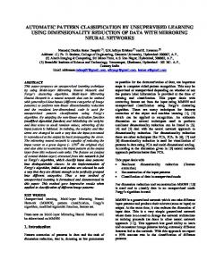
1.2 Pit patterns Diagnosis of tumorous lesions by endoscopy is always based on some sort of staging, which is a method used to evaluate the progress of cancer in a patient and to see to what extent a tumorous lesion has spread to other parts of the body. Staging is also very important for a physician to choose the right treatment of the colorectal cancer according to the respective stage. Several classification methods have been developed in the past such as Duke’s classification system, the modified Duke staging system and, more recently, the TNM staging system (Tumor, node, metastasis). Another classification system, based on so-called pit patterns of the colonic mucosa, was originally reported by Kudo et al. [16, 30]. As illustrated in figure 1.1 this classification differentiates between five main types according to the mucosal surface of the colon. The higher the type number the higher is the risk of a lesion to be malignant. While lesions of type I and II are benign, representing the normal mucosa or hyperplastic tissue, and in fact are nontumorous, lesions of type III to V in contrast represent lesions which are malignant. Lesions of type I and II can be grouped into non-neoplastic lesions, while lesions of type III to V can be grouped into neoplastic lesions. Thus a coarser grouping of lesions into two instead of six classes is also possible. There exist several studies which found a good correlation between the mucosal pit pattern and the histological findings, where especially techniques using magnifying colonoscopes led to excellent results [23, 27, 28, 29, 42, 17]. As depicted in figure 1.1 pit pattern types I to IV can be characterized fairly well, while type V is a composition of unstructured pits. Table 1.1 contains a short overview of the main characteristics of the different pit pattern types. Figure 1.2 again shows the different pit pattern types, but this time in the third dimension. This makes it easier to understand how the different pit pattern types develop over time.

2

1.2 Pit patterns

(a) Pit pattern I

(b) Pit pattern II

(c) Pit pattern IIIS

(d) Pit pattern IIIL

(e) Pit pattern IV

(f) Pit pattern V

Figure 1.1: Pit pattern classification according to Kudo et al.

(a) Pit pattern I

(b) Pit pattern II

(c) Pit pattern IIIS

(d) Pit pattern IIIL

(e) Pit pattern IV

(f) Pit pattern V

Figure 1.2: Images showing 3D views of the different types of pit pattern according to Kudo. Although at a first glance this classification scheme seems to be straightforward and easy to be applied, it needs some experience and exercising to achieve fairly good results [22, 45].

3

1 Introduction Pit pattern type I II III S III L IV V

Characteristics roundish pits which designate a normal mucosa stellar or papillary pits small roundish or tubular pits, which are smaller than the pits of type I roundish or tubular pits, which are larger than the pits of type I branch-like or gyrus-like pits non-structured pits

Table 1.1: The characteristics of the different pit pattern types.

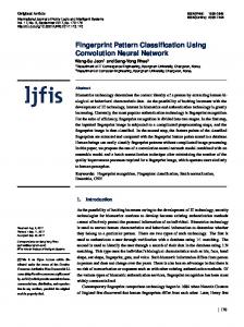
To show this, figure 1.3 contains images out of the training image set used throughout this thesis.

(a) Pit pattern I

(b) Pit pattern II

(c) Pit pattern IIIS

(d) Pit pattern IIIL

(e) Pit pattern IV

(f) Pit pattern V

Figure 1.3: Images showing the different types of pit pattern.

From these images it is not as easy anymore to tell which type of pit pattern each of these images represents. Apart from that it is important to mention that a classification solely based on pit pattern classification is not possible. There is always a final histological finding needed for the physician to decide whether a lesion in a colon is tumorous or non-tumorous.

4

1.3 Computer based pit pattern classification

1.3 Computer based pit pattern classification The motivation behind computer based pit pattern classification is to assist the physician in analyzing the colon images taken with a colonoscope just in time. Thus a classification can already be done during the colonoscopy and therefore this makes a fast classification possible. But as already mentioned above, a final histological finding is needed here too to confirm the classification made by the computer. The process of the computer based pit pattern classification can be divided into the following steps: 1. First of all as many images as possible have to be acquired. These images serve for training as well as for testing a trained classification algorithm. 2. The images are analyzed for some specific features such as textural features, color features, frequency domain features or any other type of features. 3. A classification algorithm of choice is trained with the features gathered in the last step. 4. The classification algorithm is presented some unknown image to classify. The unknown image in this context is an image which has not been used during the training step. From these steps the very important question which features to extract from the images arises. Since there are many possibilities for image features, chapter 3 will give a short overview of some possible features for texture classification. However, as the title of this thesis already suggests, the features we intend to use are solely based on the wavelet transform. Hence, before we start thinking about possible features to extract from endoscopic images, the next chapter tries to give a short introduction to wavelets and the wavelet transform.

5

1 Introduction

6

2 Wavelets Every great advance in science has issued from a new audacity of imagination. - John Dewey, The Quest for Certainty

2.1 Introduction In the history of mathematics wavelet analysis shows many origins. It was Joseph Fourier who did the first step towards wavelet analysis by doing research in the field of frequency analysis. He asserted that any 2π-periodic function can be expressed as a sum of sines and cosines with different amplitudes and frequencies. The first wavelet function developed was the Haar wavelet developed by A. Haar in 1909. This wavelet has compact support but unfortunately is not continuously differentiable, a fact, which limits its applications. The wavelet theory adopts the idea to express a function as a sum of other so-called basis functions. But the key difference between a fourier series and a wavelet is the choice of the basis functions. A fourier series expresses a function, as already mentioned, in terms of sines and cosines which are periodic functions whereas the discrete wavelet transform for example only uses basis functions with compact support. This means that wavelet functions vanish outside of a finite interval. This choice of the basis functions eliminates a disadvantage of the fourier analysis. Wavelet functions are localized in space, the sine and cosine functions of the fourier series are not. The name “wavelet” originates from the important requirement of wavelets that they should integrate to zero, “waving” above and below the x-axis. This requirement can be expressed more mathematically as Z ∞ ψ(t)dt = 0 (2.1) −∞

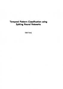
where ψ is the wavelet function used. Figure 2.1 shows some different choices for ψ. An important fact is that wavelet transforms do not have a single set of basis functions like the Fourier transform. Instead, the number of possible basis functions for the wavelet transforms is infinite. The range of applications where wavelets are used nowadays is wide. It includes signal compression, pattern recognition, speech recognition, computer graphics, signal processing, just to mention a few.

7

2 Wavelets

(a) Haar

(b) Mexican hat

(c) Sinc

Figure 2.1: Different wavelet functions ψ This chapter tries to give an introduction to the wavelet transform. A more detailed description covering also the mathematical details behind wavelets can be found in [2, 32, 46, 19, 4, 34, 24, 6].

2.2 Continuous wavelet transform The basic idea behind the wavelet theory, as already mentioned above, is to express a function as a combination of basis functions ψa,b . These basis functions are just dilated and scaled versions of a so-called mother wavelet ψ. The dilations and translations of the mother wavelet or analyzing wavelet ψ define an orthogonal basis. To allow dilation and translation the dilation parameter a and the translation parameter b are introduced. Thus the resulting wavelet function can be formulated as   1 t−b ψa,b (t) = √ ψ (2.2) a a Based on these basis functions the wavelet transform for a continuous signal x(t) with respect to the defined wavelet function can be written as   Z ∞ t−b 1 dt (2.3) T (a, b) = √ x(t)ψ a a −∞

8

2.3 Discrete wavelet transform Using equation (2.2), T (a, b) can be rewritten in a more compact way as Z ∞ x(t)ψa,b (t)dt T (a, b) =

(2.4)

−∞

This can than be expressed as an inner product of the signal x(t) and the wavelet function ψa,b (t) T (a, b) = hx, ψa,b i

(2.5)

Since a, b ∈ R this is called the continuous wavelet transform. Simply spoken equation (2.5) returns the correlation between a signal x(t) and a wavelet ψa,b .

2.3 Discrete wavelet transform The discrete wavelet transform is very similar to the continuous wavelet transform, but while in equation (2.2) the parameters a and b were continuous, in the discrete wavelet transform these parameters are restricted to discrete values. To achieve this, equation (2.2) is slightly modified   t − nb0 am 1 0 (2.6) ψm,n (t) = √ m ψ a0 am 0
1 = √ m ψ a−m (2.7) 0 t − nb0 a0 where m controls the dilation and n the translation with m, n ∈ Z. a0 is a fixed dilation step parameter greater than 1 and b0 is the location parameter which must be greater than 0. The wavelet transform of a continuous signal x(t) using discrete wavelets of the form of equation (2.7) is then Z ∞
1 Tm,n = √ m x(t)ψ a−m (2.8) 0 t − nb0 dt a0 −∞ which again can be written in a more compact way Z ∞ Tm,n = x(t)ψm,n (t)dt

(2.9)

−∞

and therefore leads to Tm,n = hx, ψm,n i

(2.10)

9

2 Wavelets For the discrete wavelet transform, the values Tm,n are known as wavelet coefficients or detail coefficients. Common choices for the parameters a0 and b0 in equation (2.7) are 2 and 1, respectively. This is known as the dyadic grid arrangement. The dyadic grid wavelet can be written as
m (2.11) ψm,n (t) = 2− 2 ψ 2−m t − n The original signal x(t) can be reconstructed in terms of the wavelet coefficients Tm,n as follows: ∞ X

x(t) =

∞ X

Tm,n ψm,n (t)

(2.12)

m=−∞ n=−∞

The scaling function of a dyadic discrete wavelet is associated with the smoothing of the signal x(t) and has the same form as the wavelet, given by
m (2.13) φm,n (t) = 2− 2 φ 2−m t − n In contrast to equation (2.1) scaling functions have the property Z ∞ Z ∞ φ0,0 (t)dt = φ(t)dt = 1 −∞

(2.14)

−∞

where φ(t) is sometimes referred to as the father scaling function. The scaling function can be convolved with the signal to produce approximation coefficients as follows: Z ∞ Sm,n = x(t)φm,n (t)dt (2.15) −∞

A continuous approximation of the signal at scale m can be generated by summing a sequence of scaling functions at this scale factored by the approximation coefficients as follows: xm (t) =

∞ X

Sm,n φm,n (t)

(2.16)

n=−∞

where xm (t) is a smoothed, scaling-function-dependent, version of x(t) at scale m. Now the original signal x(t) can be represented using both the approximation coefficients and the wavelet (detail) coefficients as follows: x(t) =

∞ X n=−∞

10

Sm0 ,n φm0 ,n (t) +

m0 X

∞ X

m=−∞ n=−∞

Tm,n ψm,n (t)

(2.17)

2.3 Discrete wavelet transform From this equation it can be seen that the original signal is expressed as a combination of an approximation of itself (at an arbitrary scale index m0 ), added to a succession of signal details from scales m0 down to −∞. The signal detail at scale m is therefore defined as ∞ X

dm (t) =

Tm,n ψm,n (t)

(2.18)

n=−∞

hence equation (2.17) can be rewritten as x(t) = xm0 (t) +

m0 X

dm (t)

(2.19)

m=−∞

which shows that if the signal detail at an arbitrary scale m is added to the approximation at that scale it results in an signal approximation at an increased resolution (m − 1). The following scaling equation describes the scaling function φ(t) in terms of contracted and shifted versions of itself: X ck φ(2t − k) (2.20) φ(t) = k

where φ(2t − k) is a contracted version of φ(t) shifted along the time axis by step k ∈ Z and factored by an associated scaling coefficient, ck , with ck = hφ(2t − k), φ(t)i

(2.21)

Equation (2.20) basically shows that a scaling function at one scale can be constructed from a number of scaling functions at the previous scale. From equation (2.13) and (2.20) and examining the wavelet at scale index m + 1, one can see that for arbitrary integer values of m the following is true:     X m 1 t 2t − m+1 − − ck φ − 2n − k (2.22) 2 2 φ m+1 − n = 2 2 2 2 2 2 · 2m k which can be written more compactly as 1 X φm+1,n = √ ck φm,2n+k (t) 2 k

(2.23)

That is, the scaling function at an arbitrary scale is composed of a sequence of shifted scaling functions at the next smaller scale each factored by their respective scaling coefficients.

11

2 Wavelets Now, that we have defined the scaling function φ, we can construct a suited wavelet function 1 X ψm+1,n = √ bk φm,2n+k (t) 2 k

(2.24)

bk = (−1)k cNk −1−k

(2.25)

where

and Nk is the number of scaling coefficients. Analogous to equation (2.21) we can express bk as bk = hφ(2t − k), ψ(t)i

(2.26)

From equation (2.24) we can see, that the wavelet function ψ can be expressed in terms of the scaling function φ. This is an important relationship which is used in the next section to obtain the filter coefficients.

2.4 Filter based wavelet transform In signal processing usually a signal is a discrete sequence. To analyze such a signal with the wavelet transform based on filters so-called filter banks are needed, which guarantee a perfect reconstruction of the signal. A filter bank consist of a low pass filter and a high pass filter. While the low pass filter (commonly denoted by h) constructs an approximation subband for the original signal, the high pass filter (commonly denoted by g) constructs a detail subband consisting of those details, which would get lost if only the approximation subband would be used for signal reconstruction. To construct a filter bank we need to compute the coefficients for the low pass filter h first. However, since the scaling equation is used to get the approximation for a signal, h can be composed by using the coefficients ck from equation (2.20): h[k] = ck

(2.27)

Now, using equations (2.24) and (2.25), we are able compute g from h: g[k] = (−1)k h[Nk − 1 − k]

(2.28)

For a discrete signal sequence x(t) the decomposition can be expressed in terms of a convolution as ya (k) = (h ∗ x)[k]

12

(2.29)

2.4 Filter based wavelet transform and yd (k) = (g ∗ x)[k]

(2.30)

where ya and yd denote the approximation and the detail subband. The discrete convolution between a discrete signal x(t) and a filter f (t) is defined as (f ∗ x)(k) =

l X

f (i)x(k − i)

(2.31)

i=0

where l is the length of the respective filter f . To avoid redundant data in the decomposed subbands, the signal of length N is downsampled to length N/2. Therefore the result of equation (2.29) and (2.30) are sequences of length N/2 and the decomposed signal has a length of N . To reconstruct the original signal x from ya and yd a reconstruction filter bank consisting ˆ and gˆ, which are the low pass and high pass reconstruction filters, is used. of the filters h Since during the decomposition the signal was downsampled, the detail and the approximation subband have to be upsampled from size N/2 to size N . Then the following formula is used to reconstruct the original signal x. ˆ ∗ ya )(t) + (ˆ x(t) = (h g ∗ yd )(t)

(2.32)

ˆ and gˆ can be computed from the previously computed decomThe reconstruction filters h position filters h and g using the following equations ˆ = (−1)k+1 g[k] h[k]

(2.33)

gˆ[k] = (−1)k h[k]

(2.34)

and

A special wavelet decomposition method without any downsampling and upsampling involved is the algorithme a` trous. This algorithm provides approximate shift-invariance with an acceptable level of redundancy. Since in the discrete wavelet transform at each decomposition level every second coefficient is discarded, this can result in considerably large shift-variances. When using the algorithme a` trous however the subbands are not downsampled during decomposition and the same amount of coefficients is stored for each subband - no matter at which level of decomposition a subband is located in the decomposition tree. As a consequence no upsampling is needed at all when reconstructing a signal.

13

2 Wavelets

2.5 Pyramidal wavelet transform While the transformation process described in section 2.4 transforms a 1D-signal, in image processing the main focus lies on 2D-data. To apply the wavelet transform on images first the column vectors are transformed, then the row vectors are transformed - or vice versa. This results in four subbands - an approximation subband and three detail subbands. In the pyramidal wavelet transform only the approximation subband is decomposed further. Thus, if repeating the decomposition step of the approximation subband again and again, the result is a pyramidal structure, no matter what image is used as input. Figure 2.2(a) shows such a pyramidal decomposition quadtree. The motivation behind the pyramidal wavelet transform is the fact that in most natural images the energy is concentrated in the approximation subband. Thus by decomposing the approximation subband again and again the highest energies are contained within very few coefficients since the approximation subband gets smaller and smaller with each decomposition step. This is an important property for image compression for example. But there are also images for which this decomposition structure is not optimal. If an image for example has periodic elements the pyramidal transform is not able anymore to concentrate the energy into one subband. A solution to this problem are wavelet packets.

2.6 Wavelet packets Wavelet packets have been introduced by Coifman, Meyer and Wickerhauser as an extension to multiresolution analysis and wavelets. In contrast to the pyramidal wavelet transform, where only the approximation subband is decomposed further the wavelet packet transform also allows further decomposition of detail subbands. This allows an isolation of other frequency subbands containing high energy which is not possible in the pyramidal transform. Due to the fact that any subband can now be decomposed further this results in a huge number of possible bases. But depending on the image data and the field of application an optimal basis has to be found. In the next sections some methods for basis selection are presented.

2.6.1 Basis selection When performing a full wavelet packet decomposition all subbands are decomposed recursively until a maximum decomposition level is reached, no matter how much information is contained within each subband. The task of basis selection is used to optimize this process by selecting a subset of all possible bases which fits as well as possible for a specific task. Depending on whether the goal is compression of digital data or data classification for example different basis selection algorithms are used. The reason for this is that there is currently

14

2.6 Wavelet packets

(a)

(b)

Figure 2.2: Pyramidal decomposition (a) and one possible best-basis wavelet packet decomposition (b) no known basis selection algorithm with has to be proven to perform well in classification tasks as well as in compression tasks. This is mainly due to the fact that the underlying principles of compression and classification are quite different. While in compression the main goal is to reduce the size of some data with as few loss as possible, the main goal in classification is to find a set of features which is similar among inputs of the same class and which differ among inputs from different classes.

2.6.1.1 Best-basis algorithm The best-basis algorithm, which was developed by Coifman and Wickerhauser [11] mainly for signal compression, tries to minimize the decomposition tree by focusing on subbands only which contain enough information to be regarded as being interesting. To achieve this, an additive cost function is used to decide whether a subband should be further decomposed or not. The algorithm can be outlined by the following steps: 1. A full wavelet packet decomposition is calculated for the input data which results in a decomposition tree. 2. The resulting decomposition tree is traversed from the leafs upwards to the tree root comparing the additive cost of the children nodes and the according parent node for each node in the tree having children nodes. 3. If the summed cost of the children nodes exceeds the cost of the according parent node the tree gets pruned at that parent node, which means that the children nodes are removed. The resulting decomposition is optimal in respect to the cost function used. The most common additive cost functions used are

15

2 Wavelets Logarithm of energy (LogEnergy) cost(I) =

N X

log∗ (s)

s = I(i)2

with

i=1

Entropy cost(I) = −

N X

s log∗ (s)

s = I(i)2

with

i=1

Lp -Norm cost(I) =

N X

|I(i)|p

i=1

Threshold cost(I) =

N X

 a

a=

with

i=1

1 if I(i) > t 0 else

where I is the input sequence (the subband), N is the length of the input, log∗ is the logfunction with the convention log(0) = 0 and t is some threshold value.

(a) Source image

(b) LogEnergy

(c) Entropy

(d) L-Norm

(e) Threshold

Figure 2.3: Different decomposition trees resulting from different cost functions using the Haar wavelet.

16

2.6 Wavelet packets

(a) Source image

(b) LogEnergy

(c) Entropy

(d) L-Norm

(e) Threshold

Figure 2.4: Different decomposition trees resulting from different cost functions using the biorthogonal Daubechies 7/9 wavelet. In figure 2.3 the resulting decomposition trees for an example image using different cost functions are shown. The image in 2.3(a) was decomposed using the Haar wavelet with a maximum decomposition level of 5. In this example the threshold value t for the threshold cost function was set to 0. In figure 2.4 again the resulting decomposition trees for different cost functions are shown. But this time the biorthogonal Daubechies 7/9 wavelet was used. The parameters used for the decomposition and the source image are the same as used to produce the decomposition trees in figure 2.3. Note the difference between the decomposition trees in figure 2.3 and 2.4. While using the threshold cost function in these examples results in quite similar decomposition trees (figure 2.3(e) and 2.4(e)), the other cost functions exhibit fairly different decomposition trees. The best-basis algorithm has proven to be well suited for signal compression but is not necessarily as good for classification problems. A further example of a basis found with the best-basis algorithm is shown in figure 2.2(b). 2.6.1.2 Tree-structured wavelet transform The tree-structured wavelet transform introduced by Chang and Kuo [10] is another adaptive decomposition method for wavelets which is very similar to the best-basis algorithm. But instead of pruning the decomposition tree in a bottom-up manner, as it is done in the best-basis algorithm, the decisions which subbands to decompose further are already made during the top-down decomposition process.

17

2 Wavelets While the best-basis algorithm is based on a full wavelet packet decomposition, the algorithm presented in [10] stops the decomposition process for a node of the decomposition tree if the subbands (i.e. the child nodes) do not contain enough information to be regarded as interesting for further decomposition. In other words this algorithm tries to detect significant frequency channels which are then decomposed further. The stopping criterion for a subband s at scale j is met if e < Cemax where e is the energy contained in the subband s, emax is the maximum energy among all subbands at scale j and C is a constant less than 1. For a small C a subband is more likely to be decomposed further than it is the case for a value near 1. 2.6.1.3 Local discriminant bases The local discriminant bases algorithm is an extension to the best-basis algorithm developed by Saito and Coifman [39] primarily focused on classification problems. The local discriminant bases algorithm searches for a complete orthonormal basis among all possible bases in a time-frequency decomposition, such that the resulting basis can be used to distinguish between signals belonging to different signal classes and therefore to classify different signals. As the time-frequency decomposition model we use the wavelet packet decomposition, but others such as the local cosine transform or the local sine transform for example can be chosen as the time-frequency decomposition method too. First of all the images are normalized to have zero mean and unit variance as suggested in [41]. This is done by applying the following formula to the input sequence: I(i) =

I(i) − µI σI

where I is the input signal sequence, µI is the mean of the input sequence N 1 X I(i), µI = N i=1

σI is the standard deviation of the input sequence v u N q uX
2 2 I(i) − µI σI = σI = t i=1

and 1 ≤ i ≤ N for an input length of N . After this preprocessing the wavelet packet decomposition is used to create a so-called time-frequency dictionary which is just a collection of all nodes in a full n-level decomposition. Then, signal energies at each node in the decomposition tree are accumulated at each

18

2.6 Wavelet packets coefficient for each signal class l separately to get a so-called time-frequency energy map Γl for each signal class l, which is then normalized by the total energy of the signals belonging to class l. This can be formulated as Γl (j, k) =

Nl X

(l) (si,k )2 /

Nl X

(l)

kxi k2

(2.35)

i=1

i=1

where j denotes the j-th node of the decomposition tree, Nl is the number of samples (l) (images) in class l, si,j,k is the k-th wavelet coefficient of the j-th subband (node) of the i-th (l)

image of class l and xi is the i-th signal of class l. This time-frequency energy map is then used by the algorithm to determine the discrimination between signals belonging to different classes l = 1, . . . , L where L is the number of total different signal classes. The discriminant power of a node is calculated using a discriminant measure D, which measures statistical distances among classes. There are many choices for the discriminant measure such as the relative entropy which is also known as the cross-entropy, Kullback-Leibler distance or I-divergence. Other possible measures include the J-divergence, which is a symmetric version of the I-divergence, the Hellinger distance, the Jenson-Shannon divergence and the euclidean distance. I-divergence D(pa , pb ) =

n X

pai log

i=1

p ai pbi

J-divergence D(pa , pb ) =

n X i=1

n

X pb pa pbi log i pai log i + pbi p ai i=1

Hellinger-distance D(pa , pb ) =

n X √

p ai −

√

pbi


2

i=1

Jenson-Shannon divergence X  n n p ai X pbi D(pa , pb ) = pai log + pbi log /2 q q i i i=1 i=1 with qi =

pai + pbi 2

19

2 Wavelets Euclidean distance D(pa , pb ) = kpa − pb k2 where pa and pb are two nonnegative sequences representing probability distributions of signals belonging to classes a and b respectively and n is number of elements in pa and pb . Thus, the discriminant measures listed above are distance measures for probability distributions and are used to calculate the discriminant power between pa and pb . To use these measures to calculate the discriminant power over L classes we use the following equation: D({pl }Ll=1 ) =

L−1 X L X

D(pi , pj )

(2.36)

i=1 j=i+1

In terms of the time frequency energy map equation (2.36) can be written as D({Γl (n)}Ll=1 ) =

L−1 X L X

D(Γi (n), Γj (n))

(2.37)

i=1 j=i+1

where n denotes the n-th subband (node) in the decomposition tree. The algorithm to find the optimal basis can be outlined as follows: 1. A full wavelet packet decomposition is calculated for the input data which results in a decomposition tree. 2. The resulting decomposition tree is traversed from the leafs upwards to the tree root comparing the additive discriminant power of the children nodes and the according parent node for each node in the tree having children nodes. To calculate the discriminant power the discriminant measure D is used to evaluate the power of discrimination of the nodes in the decomposition tree between different signal classes. 3. If the discriminant power of the parent node exceeds the summed discriminant power of the children nodes the tree gets pruned at that parent node, which means that the children nodes are removed. To obtain a fast computational algorithm to find the optimal basis, D has to be additive just as the cost function used in the best-basis algorithm. After the pruning process we have a complete orthonormal basis and all wavelet expansion coefficients of signals in this basis could be used as features already. But due to the fact that the dimension of such a feature vector would be rather high it is necessary to reduce the dimensionality of the problem such that k  n where n is the number of all basis vectors of the orthonormal basis and k is the dimension of the feature vector after dimensionality reduction.

20

2.6 Wavelet packets To reduce the dimension of the feature vector the first step is to sort the basis functions by their power of discrimination. There are several choices as a measure of discriminant power of one of the basis functions such as using the discriminant measure D on the timefrequency distribution among different classes of a single decomposition tree node, which is just the power of discrimination of one node and therefore a measure of usefulness of this node for the classification process. Another measure would be the Fisher’s class separability of wavelet coefficients of a single node in the decomposition tree, which expresses the ratio of the between-class variance to (c) the in-class variance of a specific subband si,j and can be formulated as (l) (l)
2 π mean (s ) − mean (mean (s l i l i i,j i,j )) l=1 PL (l) l=1 πl variancei (si,j )

PL

(2.38) (l)

where L is the number of classes, πl is the empirical proportion of class l, si,j is the j-th subband for the i-th image of class l containing the wavelet coefficients and meanl (·) is the mean over class l, meani (·) and variancei (·) are operations to take mean and variance for (l) the wavelet coefficients of si,j , respectively. The following equation is similar to equation (2.38), but it uses the median instead of the mean, and the median absolute deviation instead of the variance: PL (l) (l)
l=1 πl | medi (si,j ) − medl (medi (si,j )) | (2.39) PL (l) l=1 πl madi (si,j ) An advantage of using this more robust method instead of the version in equation (2.38) is that it is more resistant to outliers. Having the list of basis functions (nodes of the decomposition tree) which is sorted now, the k most discriminant basis function can be chosen for constructing a classifier by feeding the features of the remaining k subbands into a classifier such as linear discriminant analysis (LDA) [39, 3], classification and regression trees (CART) [35], k-nearest neighbours (kNN) [18] or artificial neural networks (ANN) [38]. This process can then be regarded as a training process for a given classifier, which labels each given feature vector with a class name. The classification of a given signal is then done by expanding the signal into the LDB and feeding the classifier already trained with the respective feature vector of the signal sequence to classify. The classifier then tries to classify the signal and returns the according class. After this introduction to wavelets and showing some important preliminaries regarding wavelets, we are now prepared to start thinking about possible features which might be used for the classification of pit pattern images. Hence the next chapter will present some already existing techniques regarding texture feature extraction with a focus on wavelet based methods. Chapter 4 then gives a more thorough overview regarding possible features, when the different technique are presented, which are used to test the pit pattern classification.

21

2 Wavelets

22

3 Texture classification It is not enough to do your best; you must know what to do, and then do your best. - W. Edwards Deming

3.1 Introduction If a computer program has to discriminate between different classes of images some sort of classification algorithm has to be applied to the training data during the training phase. During the classification of some unknown image the formerly trained classification algorithm is presented the new, unknown image and tries to classify it correctly. Thus the classification process mainly consist of two parts: the extraction of relevant features from images and the classification based on these features. This chapter will give a literature review, presenting approaches which mainly employ features based on wavelets presented in chapter 2. But we will also see some examples of endoscopic classification which do not use any wavelet based features. Apart from the feature extraction this chapter gives an introduction to some well-known classification algorithms.

3.2 Feature extraction 3.2.1 Wavelet based features To use wavelet based features, the image to be analyzed has to be decomposed using a wavelet decomposition method such as the pyramidal wavelet transform or wavelet packets (see chapter 2). Then, having the resulting subbands, different types of features can be extracted from the coefficients contained within the according subbands. These include the mean and standard deviation of coefficients in a subband, features based on wavelet coefficient histograms, features based on wavelet coefficient co-occurrence matrices (see section 4.2.1.1) and modeling parameters for wavelet coefficient histograms, just to mention a few. The method presented in [5], for example, uses features based on the mean and standard deviation of coefficients inside of wavelet subbands. Bhagavathy presents a wavelet-based

23

3 Texture classification image retrieval system based on a wavelet-based texture descriptor which is based upon a weighted standard deviation (WSD) descriptor. To extract the WSD texture feature vector from a gray scale image the first step is a L-level wavelet decomposition using the Haar wavelet. Then the standard deviation is calculated for the three resulting detail images of each level (HL, LH and HH) and the approximation image at level L. Additionally the mean of the approximation image is calculated. The WSD texture feature vector is then built up from these values as follows: f = {σ1LH , σ1HL , σ1HH , ν2 σ2LH , ν2 σ2HL , ν2 σ2HH , . . . , νL σLLH , νL σLHL , νL σLHH , νL σ A , µA } (3.1) with νk = 2−k+1

(3.2)

where σiLH , σiHL and σiHH are the standard deviations of the according detail subbands of level i and µA is the mean of the approximation image. The weighting factor at each level is motivated by the expectation that higher frequency subbands contain more texture information and should therefore contribute more to the WSD feature vector. The mean of the approximation image gives information about the intensity in the image. The resulting feature vector for a L-level wavelet decomposition then has a magnitude of 3L + 2. For the image retrieval process the images are first mapped from RGB space to YCrCb space to separate textural information and color information of the image. Then the WSD feature vector is calculated for each image component (Y, Cr and Cb) which results in a final feature vector containing 33 elements. This content descriptor now compactly describes both texture and color in images. One major advantage of this descriptor is the possibility to be able to give weights to the texture and color components. The approach presented in [37] is also based on the discrete wavelet transform, but it utilizes the local discriminant bases (see 2.6.1.3) to extract the optimal features for classification. Rajpoot presents a basis selection algorithm which extends the concept of “Local Discriminant Basis” to two dimensions. The feature selection is addressed by the features according to their relevance, which has a significant advantage over other feature selection methods since the basis selection and reduction of dimensionality can be done simultaneously. Since in contrast to the wavelet decomposition in a wavelet packet decomposition high frequency subbands can be further decomposed as well, this results in a huge number of possible bases. From these bases the most suitable basis for texture classification, a basis with a maximum discriminating power among all possible bases, needs to be chosen. For this purpose Rajpoot employed the concept of Local Discriminant Bases and used four different cost functions in his experiments. Namely, Kullback-Leibler divergence, JensenShannon divergence, Euclidean distance and Hellinger distance. Feature selection is done by selecting a subset out of all subbands of the wavelet packet

24

3.2 Feature extraction decomposition. This subset is composed of subbands which show a high discrimination between different classes of textures such that it highlights the frequency characteristics of one class but not the other. Once it has been ensured that the optimal basis for texture classification is chosen, the selection of most discriminant subbands can proceed by using the cost function as a measure of relevance to classification. The feature used for classification in this approach is the discriminant power of a subband (see section 2.6.1.3). Another approach based on the wavelet transform is presented by Wouver et al. in [14]. The authors describe a method which uses first order statistics as well as second order statistics to describe the characteristics of texture. The first step of the feature extraction process is a four-level wavelet frame decomposition, which is an overcomplete representation since the detail images are not subsampled at all. The resulting wavelet detail coefficients are then used for the calculation of the wavelet coefficient histograms, which capture all first order statistics and the wavelet coefficient co-occurrence matrices (see section 4.2.1.1), which reflect the second order statistics. The authors propose that a combination of these two feature sets outperforms the use of the traditionally used energy signature in terms of classification accuracy. In another paper, Wouver et al. [15] investigate the characterization of textures by taking a possible asymmetry of wavelet detail coefficient histograms into account. In this approach the image is transformed to a normalized gray level image which is then decomposed using a four-level wavelet decomposition. For the resulting detail subbands the multiscale asymmetry signatures (MAS) are calculated as follows: Z ∞ |hni (u) − hni (−u)|u du (3.3) Ani = 0

where hni is the wavelet coefficient histogram for the i-th detail subband of the n-th decomposition level. For perfectly symmetric textures this value equals 0, whereas for asymmetric textures this value represents the degree of asymmetry. These MAS are calculated for each detail subband which results in a feature vector E containing the energy signatures. Additionally a second feature vector A+E containing the energy signatures and the asymmetry signatures is computed. These two feature vectors are then compared in terms of the classification error rate during the tests performed. This approach shows that texture classification can indeed be improved by also using asymmetry signatures, which however are very data-dependent since they are only of value for textures which exhibit asymmetry on a particular decomposition scale. A method using the extraction of histogram model parameters is presented in [12]. Cossu describes a method to discriminate different texture classes by searching for subbands with multimodal histograms. These histograms are then modeled using a model which is parameterized by the following data: a dyadic partition of one quadrant of the Fourier domain, T , which, given a mother wavelet, defines a wavelet packet basis; a map from T to the set of the three different models used; a map from T to the space of model parameters of each subband.

25

3 Texture classification By approximating the used model to a subband histogram, the respective parameters of the model are evaluated and can be used as features for a classification process. Another approach by Karkanis et al. [25], which is already focused on the classification of colonoscopic images, is based on a feature extraction scheme which uses second order statistics of the wavelet transformation of each frame of the endoscopic video. These features are then used as input to a Multilayer Feed Forward Neural Network (MFNN). As already proposed in other publications a major characteristic to differentiate between normal tissue and possible malignant lesions is the texture of the region to examine. Therefore the classification of regions in endoscopic images can be treated as a texture classification problem. For this texture classification process this approach uses the discrete wavelet transform (DWT) with Daubechies wavelet bases to extract textural feature vectors. Using the DWT a one-level wavelet decomposition is performed resulting in four wavelet subbands which are then used to obtain statistical descriptors for the texture in the region being examined. The statistical descriptors are estimated over the co-occurrence matrix (see section 4.2.1.1) for each region. These co-occurrence matrices are calculated for various angles (0◦ , 45◦ , 90◦ and 135◦ ) with a predefined distance of one pixel in the formation of the co-occurrence matrices. Based on these matrices four statistical measures are calculated which provide high discrimination accuracy. Namely angular second moment, correlation, inverse difference moment and the entropy. Calculating these four measures for each subband of the one-level wavelet decomposition, results in a feature vector containing 16 features for each region which is then used as input for the MFNN. An implementation of this approach along with classification results is documented in [33]. The methods in [31] and [43] are very similar to this method but slightly differ in the way features are extracted. While the approach by Karkanis et al. is based on co-occurrence matrix features of all subbands resulting from the wavelet decomposition, in [43] only the subband whose histogram presents the maximum variance is chosen for further feature extraction. The last method presented here using wavelet based features can be found in [26]. Karkanis et al. describe a method which first decomposes the image into the three color bands according to the RGB color model. Each of the resulting color bands is then scanned using a fixed size sliding squared window. The windows of this process are then transformed using a discrete three-level wavelet transform. Since the texture features are best represented in the middle wavelet detail channels only the detail subbands of the second level of the decomposition are considered for further examination. Since this sliding window wavelet decomposition is done for each color channel this step results in a set of nine subimages for each sliding window position. For all nine subimages the co-occurrence matrices in four directions (0◦ , 45◦ , 90◦ and 135◦ ) are calculated to obtain statistical measures which results in a set of 36 matrices. The four statistical measures used are the same as in [25], namely, angular second moment, correlation, inverse difference moment and entropy. This results in a feature vector containing 144 components.

26

3.2 Feature extraction Finally the covariances between pairs of values out of these 144 elements are calculated which results in a 72-component vector which is called the color wavelet covariance (CWC) feature vector. This CWC feature vector is then used for the classification of the image regions.

3.2.2 Other possible features for endoscopic classification The method presented by Huang et al. in [13], describes a computerized diagnosis method to analyze and classify endoscopic images of the stomach. In this paper the first step is the selection of regions of interest (ROIs) by a physician. This is done for three images, one each from the antrum, body and cardia of the stomach. These ROIs are then used for further examination for which the authors developed image parameters based on two major characteristics, color and texture. The image parameters compromising the color criterion were further defined for gray-scale intensity and the components of red, green and blue color channels of an image. For each sub-image three statistical parameters were derived: the maximum, the average and extension, indicating the maximum value, mean value and distribution extent of the histogram in the sub-image. Thus the result was a total of 12 (4 × 3) color features. To obtain the texture parameters, the same features as used in the color feature computation were introduced for the texture. Additionally three texture descriptors were generated based on sum and difference histograms in the horizontal and vertical direction. These descriptors are contrast, entropy and energy. This further refinement of texture features results in a total number of 72 (4 × 3 × 3 × 2) texture features and therefore in a total number of 84 features (color and texture). Another method also focused on the computer based examination of the colon is presented in [44]. Instead of examining an image in total texture units (TU’s) are introduced. A TU characterizes the local texture information for a given pixel. Statistics of all TUs over the whole image can then be used to gather information about the global texture aspects. Each entry of a TU can hold one of the following three values: 0 if the value of the center pixel is less than the neighbouring pixel value 1 if the value of the center pixel is equal to the neighbouring pixel value 2 if the value of the center pixel is greater than the neighbouring pixel value Having three possible values for each entry of a TU, the neighbourhood of a pixel covering eight pixels can represent one out of 38 (6561) possible TU’s. The texture unit number is then calculated from the elements of a texture unit by using the formula (δ×δ)−1

NT U =

X

Ei × δ i−1

(3.4)

i=1

27

3 Texture classification where Ei is the i-th element of the TU and δ is the length and width of the neighbourhood measured in pixels (3 in this approach). Using this texture unit numbers a texture spectrum histogram for an image can be calculated revealing the frequency distribution of the various texture units. Such a texture spectrum is calculated for the image components Intensity, Red, Green, Blue, Hue and Saturation. These spectra are then used to obtain statistical measures such as energy, mean, standard-deviation, skew, kurtosis and entropy. Apart from the textural descriptors color-based features are extracted too. This is motivated by the fact that malignant tumors tend to be reddish and more severe in color than the surrounding tissue. Benign tumors on the other hand exhibit less intense hues. Based on these properties color features for various image components (Intensity, Red, Green, Blue, Hue and Saturation) are extracted. This is done by specifying threshold values L1 and L2 . Then all histogram values for the intensities from 0 to L1 are summed up to form S1 . Similarly all histogram values for the intensities between L1 and L2 are summed up to form S2 . The color feature for the according image component is then S2 divided by S1 .

3.3 Classification In the previous section some methods used to extract features from images were presented. Without any classification process however these features would be meaningless. In the following we present the methods used for classification in the approaches presented in the previous section which are the k-NN classifier (k-NN), artificial neural networks (ANNs) and support vector machines (SVMs).

3.3.1 k-NN The k-NN classifier is one of the simplest classifiers but already delivers promising results. This classifier has been used for example in [14] for evaluation of the features’ discriminative power. To apply the k-NN classifier first of all feature vectors for each sample to classify must be calculated. Then the k-NN algorithm searches for the k training samples for which the respective feature vectors have the smallest distances to the feature vector to be classified according to some distance function such as the euclidean distance. The euclidean distance D between two feature vectors f and g is defined as follows: D(f, g) =

sX max

(fi − gi )2

(3.5)

i=1

The class label which is represented most among these k images is then assigned to unclassified data sample.

28

3.3 Classification In figure 3.1 an example 2-dimensional feature space is shown. The filled circles represent feature vectors of a class A, while the outlined circles represent feature vectors of a second class, B. The filled quad is the feature vector for an image sample which has to be classified. If we choose now a k-value of 2 for example the unknown sample will be assigned to class A. However, if the value of k is set to a higher value, we can clearly see, that the unknown sample has more nearest neighbours in class B, and will thus be assigned to the second class. This little example illustrates very well, that different values of k may result in different classification results - especially if more classes are used.

Figure 3.1: The k-NN classifier for a 2-dimensional feature space. The method presented in [5] uses a simple similarity measure. This measure is obtained by computing the L1 -distance between the 33-dimensional feature vectors of two images. As already pointed out in section 3.2.1, in this approach such a feature vector contains a weighted standard deviation descriptor, which is built up from the weighted standard deviations in the detail subbands and the mean of the approximation image resulting from a pyramidal wavelet decomposition. The distance between two feature vectors f and g of two images is then defined as follows:

D(f, g) =

1 1 1 |f1 − g1 | + |f2 − g2 | + . . . + |f33 − g33 | σ1 σ2 σ33

(3.6)

where σi is the standard deviation of the i-th element of the feature vector.

3.3.2 ANN In [25], [43], [33] and [31] the artificial neural network classifier was used for classification. Since the latter three approaches are based on the same paper, they all use a Multilayer Feed Forward Neural network (MFNN). The MFNN used is trained using the momentum backpropagation algorithm which is an extension of the standard backpropagation algorithm.

29

3 Texture classification After the MFNN has been trained successfully it is able to discriminate between normal and abnormal texture regions by forming hyperplane decision boundaries in the pattern space. In [43], [33] and [31] the ANN is fed with feature vectors, which contain wavelet coefficient co-occurrence matrix based features based on the subbands resulting from a 1-level DWT. Karkanis et al. use in [25] a very similar approach, but consider only the subband exhibiting the maximum variance for feature vector creation. According to the results in the publications the classification results are promising since the system used has been proven capable to classify and locate regions of lesions with a success rate of 94 up to 99%. The approach in [44] uses an artificial neural network for classification too. The color features extracted in this approach are used as input for a Backpropagation Neural Network (BPNN) which is trained using various training algorithms such as resilient propagation, scaled conjugate gradient algorithm and the Marquardt algorithm. Depending on the training algorithm used for the BPNN and the combination of features which is used as input for the BPNN this approach reaches an average classification accuracy between 89 and 98%. The last of the presented methods also using artificial neural networks is presented in [13]. The 84 features extracted with this method are used as input for a multilayer backpropagation neural network. This results in a classification accuracy between 85 and 90%.

3.3.3 SVM The SVM classifier, further described in [7, 20], is another, more recent technique for data classification, which has already been used for example by Rajpoot in [36] to classify texture using wavelet features. The basic idea behind support vector machines is to construct classifying hyperplanes which are optimal for separation of given data. Apart from that the hyperplanes constructed from some training data should have the ability to classify any unknown data presented to the classifier as well as possible. In figure 3.2(a) an example 2-dimensional feature space with linear separable features of two classes A (filled circles) and B (outlined circles) is shown. The black line running through the feature space is the hyperplane separating the feature space into to half spaces. Additionally on the left side of the hyperplane as well as on the right side of the hyperplane two other lines can be seen - drawn in gray in figure 3.2. These lines are boundaries, which have the same distance h to the separating hyperplane at any point. These boundaries are important, as feature vectors are allowed to be on the boundaries, but not inside them. Therefore all feature vectors must always satisfy the constraint, that the distances to the hyperplane are always equal or greater than h. Since there are many classifying hyperplanes possible the SVM algorithm now tries to maximize the value of h, such that only one possible hyperplane remains.

30

3.3 Classification

(a) linear separable

(b) not linear separable

Figure 3.2: The SVM classifier for two different 2-dimensional feature spaces. The feature vectors lying on the boundary are called support vectors, hence the name support vector machines. If all feature vectors were removed except the support vectors, the resulting classifying hyperplane will remain the same. This is why those feature vectors are called support vectors. SVM training For a classification problem using two classes the training data consists of feature vectors ~xi ∈ Rn and the associated class labels yi ∈ {−1, 1} where n is the number of elements in the feature vectors. All feature vectors which lie on the separating hyperplane satisfy the equation ~xi w ~ +b=0

(3.7)

where w ~ is the normal to the hyperplane and b/kwk ~ is the perpendicular distance from the hyperplane to the origin. The training data must satisfy the equations ~xi w ~ +b≥1

for

yi = 1

(3.8)

~xi w ~ +b≤1

for

yi = −1

(3.9)

and

which can be combined into yi (~xi w ~ + b) − 1 ≥ 0

∀i

(3.10)

We now consider the feature vectors which lie on the boundaries and satisfy the following equations ~xi w ~ +b=1

for

yi = 1

(3.11)

31

3 Texture classification and ~xi w ~ + b = −1

for

yi = −1

(3.12)

Using the euclidean distance between a vector ~x and the hyperplane (w, ~ b) d(w, ~ b; ~x) =

|~xw ~ + b| kwk ~

(3.13)

and the constraints imposed by equations (3.11) and (3.12), the distance between the feature vectors which are closest to the separating hyperplane is defined by h=

1 kwk ~

(3.14)

Thus, the optimal hyperplane can be found by maximizing h, which is equal to minimizing kwk ~ 2 and satisfying the constraint defined by equation (3.10). Nonlinear problems The method described above works well for problems which are linear separable. But as depicted in figure 3.2(b), many problems are not linear separable. The boundaries are no longer lines, like in figure 3.2(a), but curves. In the nonlinear case the main problem is that the separating hyperplane is no longer linear which imposes computational complexity to the problem. To overcome this problem the SVM classifier uses the Kernel trick. The basic idea is to map the input data to some higher dimensional (maybe infinite) euclidean space H using a mapping function Φ. Φ : Rn → H

(3.15)

Then the SVM finds a linear separating hyperplane in this higher dimensional space. Since the mapping can be very costly a kernel function K is used. K(~ xi , x~i ) = Φ(~ xi ) · Φ(x~j )

(3.16)

Using K we need never to know explicitly what Φ looks like, but only use K. Some commonly used choices for the kernel function K are Linear K(xj , xj ) = xTi xj

(3.17)

Polynomial K(xj , xj ) = (γxTi xj + r)d

32

with

γ>0

(3.18)

3.3 Classification Radial basis function (RBF) K(xj , xj ) = e−γkxi −xj k

2

with

γ>0

(3.19)

Sigmoid K(xj , xj ) = tanh(γxTi xj + r)

with

γ>0

(3.20)

where γ, r and d are kernel parameters. Multi-class case So far we only focused on the two-class case. To handle the multiclass case as well the classification has to be extended in some way. An overview of possible methods to handle more classes with the SVM can be found in [21]. Here we present the one-against-one approach only, since this is the method used in libSVM [8]. This method creates k(k − 1)/2 classifiers, where k is the number of different classes. Each of these classifiers can then be used to make a binary classification between some classes ca and cb where a, b ∈ {1, . . . , k} and a 6= b. Now, each binary classification is regarded as voting. An input vector ~xi , which has to be classified, is classified using each of the binary classifiers. This results in a class label, whose according voting is incremented by one. After ~xi has been classified with all of the k(k − 1)/2 binary classifiers, the class with the maximum number of votes is assigned to ~xi .

33

3 Texture classification

34

4 Automated pit pattern classification In order to succeed, your desire for success should be greater than your fear of failure. - Bill Cosby

4.1 Introduction Based on the preliminaries introduced in the last two chapters this chapter now presents methods we developed for an automated classification of pit pattern images. We describe a few techniques and algorithms to extract features from image data and how to perform a classification based on these features. Additionally this chapter introduces two classification schemes without any wavelet subband feature extraction involved.

4.2 Classification based on features The methods presented in this section first extract feature vectors from the images used, which are then used to train classifiers. The used classifiers and the process of classifier training and classification is then further described in section 4.4.

4.2.1 Feature extraction 4.2.1.1 Best-basis method (BB) In section 2.6.1 two different methods for basis selection have been presented. The classification scheme presented in this section is based on the best-basis algorithm, which, as already stated before, is primarily used for compression of image data. This approach however uses the best basis algorithm to try to classify image data. During the training process all images in IT are decomposed to obtain the wavelet packet coefficients for each image. Additionally during the decomposition some cost information is stored along with each node of the respective quadtree. This cost information is based on the chosen cost function and is used to determine the importance of a subband for the

35

4 Automated pit pattern classification feature extraction. This is important since during the feature extraction process the question arises, which subbands to choose to build the feature vector from. If the number of subbands for an image I is denoted by sI the maximum number of subbands which can be used to extract features smax from each of the images is smax = min sIi

(4.1)

1 0 ⇔ T1 6= T2

(4.38)

d(T1 , T2 ) = 0 ⇔ T1 = T2

(4.39)

d(T1 , T2 ) = d(T2 , T1 )

(4.40)

Therefore this distance between two quadtrees can be used to express the similarity between two quadtrees.

46

4.3 Structure-based classification 4.3.2.6 The distance function We can now represent each node vi in the quadtree by its unique value ui which is a unique number for the path to the node too as shown in section 4.3.2.4. Thus we now create the unordered sets of unique values for the trees T1 and T2 which are denoted by LT1 and LT2 defined as LT1 = {u1j |1 ≤ j ≤ n1 }

(4.41)

where n1 is the number of nodes in T1 and u1j is the unique number for the j-th node of T1 subtracted from 5ml+1 . The definition of LT2 is similar LT2 = {u2j |1 ≤ j ≤ n2 }

(4.42)

where n2 is the number of nodes in T2 and u2j is the unique number for the j-th node of T2 subtracted from 5ml+1 . ml is the maximum quadtree depth level among the two quadtrees to compare. Having this set we now can compare them for similarity and calculate a distance. To compare the quadtrees T1 and T2 we compare the lists LT1 and LT2 for equal nodes. To do this for each element u1j we look into LT2 for a u2k such that u1j = u2k

with

1 ≤ j ≤ n1

and

1 ≤ k ≤ n2

(4.43)

Apart from that we introduce the value t1 and t2 which are just the sum over all unique values of the nodes of T1 and T2 respectively. Additionally the value tmax is introduced as the maximum of t1 and t2 . This can be written as: t1 =

n1 X

u1j

(4.44)

u2j

(4.45)

j=1

t2 =

n2 X j=1

tmax = max(t1 , t2 )

(4.46)

If we do not find a u1j and a u2k satisfying equation (4.43) we calculate a similarity value sv using the following formula sv1 =

S X

u1z

(4.47)

z=1

47

4 Automated pit pattern classification where S is the number of different nodes in the two trees and u1z is the z-th node value which is only contained in the first quadtree subtracted from 5ml+1 . The same procedure is done for all nodes in the second tree. We sum up all unique node values of the second tree which are not contained within the first quadtree.

sv2 =

S X

u2z

(4.48)

z=1

The final similarity value is then sv = sv1 + sv2

(4.49)

Finally this similarity value is normalized to always be between 0 and 1. This is done by dividing sv by the maximum difference which can occur in terms of the unique node values. This results in the final formula for sv: sv =

sv1 + sv2 t1 + t2

(4.50)

It is obvious that sv is 0 for equal trees since then the expression sv1 + sv2 equals zero. And it is also obvious that sv can never exceed 1, since if all nodes are different sv1 + sv2 becomes t1 + t2 which results in a similarity value of 1. This function already satisfies the requirement of the distance function from equation (4.40) for equal trees to be 0, thus the final distance can be formulated as d(T1 , T2 ) = sv

(4.51)

This distance in now in the range between 0 (for equal trees) and 1 for completely different trees. Apart from that the distance has the property that differences in the first levels of the quadtree contribute more to the distance than differences in the deeper levels. This is due to the fact that the unique numbers contained within LT1 and LT2 get smaller down the tree. The biggest value is therefore assigned to the root node of the trees. Figures 4.2(b)-(e) show some example quadtrees for which the distances to the tree in figure 4.2(a) have been measured. The resulting distances listed in table 4.1 clearly show, that, as intended, differences in the upper levels of a quadtree contribute more to the distance than differences in the lower levels.

4.3.3 Distance by decomposition strings This approach measures the distance between two quadtrees by creating a decomposition string for each tree and comparing these strings for equal string sequences.

48

4.3 Structure-based classification

(a) tree A

(b) tree B1

(c) tree B2

(d) tree B3

(e) tree B4

Figure 4.2: Different example quadtrees for distance measurement tree B1 B2 B3 B4

distance 0,1408 0,0711 0,0598 0,5886

Table 4.1: Distances to tree A according to figure 4.2 using “distance by unique nodes”

4.3.3.1 Creating the decomposition string A decomposition string - in this context - is a string representation of a quadtree which is obtained by an preorder traversal of the quadtree. Let DS be the decomposition string of a quadtree T , which is initialized as an empty string. Then, during the traversal, for each node a ’1’, ’2’, ’3’ or ’4’ is appended to the string, if the first, the second, the third or the fourth child node is further subdivided, which means it contains more child nodes. Additionally an ’U’ is appended to the string if there are no more subdivisions in the child nodes and the traversal goes back one level towards the root. Figure 4.3 shows an example quadtree which results in the decomposition string 112UU32UUU2U312UU33UU43UUU434UU44UUU where the numbering from equation (4.33) is used. Using this procedure the decomposition strings DS1 and DS2 for two given quadtrees T1 and T2 are created.

49

4 Automated pit pattern classification

Figure 4.3: An example quadtree 4.3.3.2 The distance function Using DS1 and DS2 from above, we can now determine the similarity of the quadtrees T1 and T2 by comparing the according decomposition strings. This is done by comparing the strings character by character. As long as the strings are identical we know that the underlying quadtree structure is identical too. A difference at some position in the strings means that one of the strings has further child nodes where the other quadtree has no child nodes. When such a situation arises the decomposition string which contains more child nodes is scanned further until the string traversal reaches again the quadtree position of the other quadtree node which has no more child nodes. During this process for each character of the first string the difference value dv is updated according to the depth level of the different child nodes as follows: dv = dv +

1 d

(4.52)

where d is the depth of the child nodes not contained within the other quadtree. This process is repeated until DS1 and DS2 are scanned until their ends. dv then represents the number of different nodes with the according depth levels taken into account. Therefore a difference in upper levels of the quadtrees contributes more to the difference value than a difference deeper in the quadtree. Finally, to clamp the distance value between 0 and 1 the resulting difference value is divided by the sum of the lengths of DS1 and DS2 . The final distance can then be written as Pn 1 d(T1 , T2 ) =

50

i=1 di

|DS1 | + |DS2 |

(4.53)

4.3 Structure-based classification tree B1 B2 B3 B4

distance 0,1 0,0833 0,0583 0,8552

Table 4.2: Distances to tree A according to figure 4.2 using “distance by decomposition strings”

where n is the number of different nodes among the two quadtrees T1 and T2 and di is the depth level of the i-th different node. It is obvious that the distance for equal trees is 0 since in that case the sum is zero. It can also easily be seen that the distance for two completely different quadtrees never exceeds 1 since for two completely different quadtrees n becomes |DS1 | + |DS2 | which can also be written as Pn 1 d(T1 , T2 ) =

i=1 di

n

(4.54)

Since d1i is always less than 1 it is easy to see that the upper part of the fraction is always less than n. Therefore the distance is always less than 1. In table 4.2 the resulting distances according to figure 4.2 using “distance by decomposition strings” are shown. Again, just like the previous method, the results in the table clearly show, that, as intended, differences in the upper levels of a quadtree contribute more to the distance than differences in the lower levels. Compared to the distances in table 4.1, the results in table 4.2 are quite similar as long as the number of differences between two trees is low. But the more differences between two trees are present, the more different are the distance values between the two presented methods. The method based on decomposition strings shows significantly higher distance values if there are many differences between the trees.

4.3.3.3 Best basis method using structural features (BBS) This method is very similar to the best-basis method presented section 4.2.1.1 in that it is also based on the best-basis algorithm. But in contrast to the best-basis method, this method uses feature extractors which are not based on the coefficients of the subbands resulting from a wavelet decomposition but on the decomposition structures resulting from the best-basis algorithm. For this we developed three distinct feature extractors.

51

4 Automated pit pattern classification Unique node values (FEUNV) The first feature extractor constructs a feature vector for a given decomposition from the unique node values stored along with each subband (see 4.3.2). This feature extractor limits the number of subbands to use too, just like explained at the beginning of section 4.2.1.1. Thus a feature vector created by this feature extractor can be written as Fi = {U1 , U2 , . . . , Usmax }

(4.55)

where Uj denotes the unique node value of the j-th leaf node of Ti chosen to be in the feature vector (based on a cost information) and smax is the number of subbands to be used for the feature vector. For this feature extraction we again use the dominance tree extension to guarantee that all created feature vectors contain the same subbands in the same order. However, if a tree T1 contains a unique node value v which is not present among the other trees the according feature vector entry in the feature vectors for all other trees is set to 0.

(a)

(b)

Figure 4.4: Illustration of the feature vector equalization for FEUNV This process is illustrated in figure 4.4. In figure 4.4(a) we see feature vectors for some images 1 to n. As we notice, each of these feature vectors contains a feature vector entry

52

4.3 Structure-based classification (unique node value in this context), which is not present among the other feature vectors (denoted by v, w, x and y in the colored boxes). Since the feature vectors are not compareable in this form, a zero is inserted at each position, where a feature vector is missing a unique node value which is present in another feature vector. The resulting feature vectors are shown in figure 4.4(b). Now, the unique node values are located at the same positions among all feature vectors and the feature vectors can be compared by some distance metric. When using this feature extractor along with the k-NN classifier, the distance metric used to calculate the distances between the feature vectors is the euclidean distance metric already presented in equation (3.5). For example the distance between the feature vectors for images 1 and 2 presented in figure 4.4(b) along with euclidean distance metric would then result in the following distance D(f1 , f2 ) = v 2 + w2

(4.56)

where f1 and f2 are the first two feature vectors from figure 4.4(b). Tree structure (FETS) This feature extractor is very similar to the feature extractor presented in the previous paragraph since it is based on the unique node values too. But instead of limiting the number of subbands to use for feature vector generation, this feature extractor always uses the complete decomposition tree for the process of feature vector creation. A feature vector for a decomposition tree Ti can be written as Fi = {U1 , U2 , . . . , Un }

(4.57)

where Uj denotes the unique node value of the j-th leaf node of Ti and n is the total number of leaf nodes in Ti . Since this feature extractor uses all subbands of a decomposition tree to construct the feature vector from the dominance tree extension is not needed. But due to the nature of the best-basis algorithm it is also possible, like it was the case for the FEUNV feature extractor, that some feature vector contains a unique node value, which is not present among the other feature vectors. Thus, again the process illustrated in figure 4.4 is applied to the feature vectors before they are passed into any classifier. Again, if this feature extractor is used along with the k-NN classifier, the distance metric is the euclidean distance metric from equation (3.5). Tree distances (KNNTD) The last structural feature extractor we developed, uses the quadtree structures resulting from the best-basis algorithm directly to compute the k nearest neighbours in the k-NN algorithm. Thus we search for the k nearest neighbours with respect to the decomposition trees which can be regarded here as feature vectors, along with a quadtree distance metric. As quadtree distance metric we use the “distance based on unique node values” here (see section 4.3.2)

53

4 Automated pit pattern classification

4.3.4 Centroid classification (CC) Similar to the best-basis method presented in section 4.2.1.1 this method is based on the calculation of the best wavelet packet basis too. But in contrast to the best-basis method this method is not based on features extracted from the subbands resulting from the wavelet packet decomposition but on the quadtrees resulting from the wavelet packet decomposition. The idea behind this method is the question whether images decomposed using the wavelet packets algorithm in conjunction with the best-basis algorithm result in decomposition trees which can be further used for classification. A perfect classification would then be possible if trees of one image class are more similar than trees resulting from images of different classes. In other words, the similarity between trees of the same class must be much higher than the similarity of trees of different classes to be able to perform some useful classification. The similarity of two quadtrees can be expressed by the distance between them as explained in section 4.3.1. It is worthwhile to mention that having a method to express the distances between two quadtrees we could easily use that distance measure for a k-NN classification. This is exactly what the feature extractor KNNTD (see section 4.3.3.3 above) does. Since we know the classes for all training images, for an unknown test image we create the respective bestbasis decomposition tree and calculate the quadtree distances to all trees of the training images. The class, which dominates over the k nearest training images is then assigned to the unknown training image. Now, having a method to express the distance between two quadtrees and a set of images IT used for training, first of all the distances between all possible pairs of quadtrees of images out of this set are calculated as follows di,j = d(Ti , Tj )

i, j ∈ {1, . . . , n}

(4.58)

where Ti and Tj are the decomposition trees of the i-th and the j-th image respectively, n is the number of images in IT and d is the quadtree distance metric used. ITc is the subset of IT which contains all images of class c. IT = IT1 ∪ IT2 ∪ · · · ∪ ITC

(4.59)

where C is the total number of classes of images. The trees Ti and Tj , as stated above, are the result of the best-basis algorithm and are the optimal basis for the respective images in respect to a certain cost function such as the ones listed in section 4.2.1.1. The distances di,j obtained above are now used to construct a distance matrix D of size n × n with dTi ,Ti = 0

54

∀i = 1, . . . , n

(4.60)

4.3 Structure-based classification since dTi ,Ti is just the distance of a quadtree of an image to itself, which must by definition of a metric always be 0. Therefore D is   0 dT1 ,T2 . . . dT1 ,Tn  dT ,T 0 . . . dT2 ,Tn   2 1  D =  .. .. ..  . .  . . . .  dTn ,T1 dTn ,T2 . . . 0 This matrix then contains the quadtree distances (similarities) between all possible pairs of images out of the training image set. For each class c the matrix contains a submatrix Dc which contains the distances between all images belonging to class c. Therefore D can also be written as   0 dT11 ,T12 . . . dT11 ,T1n . . . dT11 ,TC1 . . . dT11 ,TCn  dT1 ,T1 0 . . . dT12 ,T1n . . . dT12 ,TC1 . . . dT12 ,TCn  2 1   .. .. .. .. .. .. ..   .. . . . . . . . .      dT1n ,T11 dT1n ,T12 . . . 0 . . . dT1n ,TC1 . . . dT1n ,TCn   D= .. .. .. .. .. .. .. ..   . . . . . . . .    d 0 . . . dTC1 ,TCn   TC1 ,T11 dTC1 ,T12 . . . dTC1 ,T1n . . .    . . . . . . . . .. .. .. .. .. .. .. ..   dTCn ,T11 dTCn ,T12 . . . dTCn ,T1n . . . dTCn ,TC1 . . . 0 where dTij ,Tkl is the distance between the j-th image (quadtree) of class i and the l-th image (quadtree) of class k. Figure 4.5(a) shows an example distance matrix for the two-class case. This example shows a perfect distance matrix with very small intra-class distances (black boxes) and very high inter-class distances (white boxes). In reality however, a distance matrix is more likely to look like the one illustrated in figure 4.5(b), since the trees for different images from a specific class hardly will be totally identical in real-world applications. As can been seen in figure 4.5 and following from equation (4.40) the distance matrices are all symmetric. Having calculated the matrix D the next task is to find the centroid of each class. A centroid of a class c in this context is the training image out of ITc which has the smallest average distance to all other images of class c. In other words, it is now necessary to find the image of class c to which all other images of class c have the smallest distance in respect to the chosen quadtree distance metric. After the centroids of all classes have been found the classification process can now take place. To classify an arbitrary image first of all the image is decomposed using the wavelet packets transform to get the respective decomposition tree. It is important to note that for classification the same cost function has to be used for pruning the decomposition tree as was used during the training phase for all training images. Then the distances of the resulting decomposition tree to the decomposition trees of the centroids of all possible classes are

55

4 Automated pit pattern classification

(a) Perfect

(b) Noisy

Figure 4.5: Distance matrices for the two-class case calculated. The class which is assigned to the image to classify is the one which has the centroid with the smallest distance to the input image according to the respective decomposition trees.

4.3.5 Centroid classification based on BB and LDB (CCLDB) Like the previous method, this method does not use any wavelet based features too, although, in contrast to the previous method, it is based on the best-basis algorithm and the LDB algorithm. This approach uses the BB and the LDB just for the creation of wavelet decomposition trees. First of all the LDB is calculated for the training images which results in a LDB tree TLDB . Then, using the best-basis algorithm, the decomposition trees Ti for all training images based on some cost function are calculated. Based on these decomposition information, for each training image Ii a distance vector Di is calculated: Di = dv(Ti , TLDB )

(4.61)

where dv is a function, which returns a vector containing all subband ids which are not equal among the two trees passed as arguments. In other words the distance vector contains all subband ids which are present either in Ti or TLDB but not in both trees. Thus the distance vectors represent the differences between the LDB tree and the trees for the images in terms of the tree structure. Then, based on the distance vectors of the images, a distance matrix D can be calculated. The matrix D is similar to the one described in section 4.3.4, but the matrix now contains the euclidean distances between the difference vectors instead of the distances between the

56

4.4 Classification decomposition trees. Therefore D is 

0

 dD1 ,D1 2 1  ..  .    dD1n ,D11 D= ..  .   d  DC1 ,D11  ..  . dDCn ,D11

dD11 ,D12 0 .. .

. . . dD11 ,D1n . . . dD12 ,D1n .. ... .

. . . dD11 ,DC1 . . . dD12 ,DC1 .. .. . .

dD1n ,D12 .. .

... .. .

. . . dD1n ,DC1 . . . dD1n ,DCn .. .. .. .. . . . . ... 0 . . . dDC1 ,DCn .. .. .. .. . . . . . . . dDCn ,DC1 . . . 0

0 .. .

dDC1 ,D12 . . . dDC1 ,D1n .. .. .. . . . dDCn ,D12 . . . dDCn ,D1n

. . . dD11 ,DCn . . . dD12 ,DCn .. .. . .

             

where dDij ,Dkl now is the euclidean distance between the j-th image (distance vector) of class i and the l-th image (distance vector) of class k. Then similar to section 4.3.4, the centroids for all classes can be calculated. But in this approach the centroids are not decomposition trees anymore, but distance vectors. Thus, a centroid in this context is the distance vector of the image of class c, which has the smallest average euclidean distance to all other distance vectors of class c. Once the centroids have been calculated, the classification is done by first decomposing an arbitrary test image IT into the according decomposition tree TT using the best-basis algorithm. Then the distance vector DT between the decomposition tree TT and the LDB tree TLDB is calculated. Having calculated the distance vector, the class of the closest centroid can be assigned to the image TT , where the closest centroid is the one having the smallest euclidean distance to DT .

4.4 Classification In this section we present the two concrete classifiers used in this thesis - namely the knearest neighbour classifier and the support vector machines.

4.4.1 K-nearest neighbours (k-NN) The k-NN classifier (see section 3.3.1) was chosen due to its simplicity when it comes to implementation. And yet this classifier already delivers promising results. To apply the k-NN classifier to the data first of all the feature vector Fα for the image Iα to classify is calculated. Then the k-NN algorithm searches for the k training images for which the respective feature vectors have the smallest distances to Fα according to some distance function such as the euclidean distance. The class label which is represented most among these k images is then assigned to the image Iα .

57

4 Automated pit pattern classification Throughout this thesis an extended version of the euclidean distance metric from equation (3.5) is used: d(Fa , Wa , Fb , Wb ) =

sX max

(Fa (i)Wa (i) − Fb (i)Wa (i))2

(4.62)

i=1

where Wa and Wb are weighting vectors for the according feature vectors. The weights in these vectors are derived from the cost information obtained by a wavelet decomposition. The motivation behind using a weighted version of the euclidean distance is that feature vector entries associated with large weights (features from subbands with high energy for example) should contribute more to the distance the more these entries differ among different feature vectors. However, regarding our test results presented in chapter 5 it does not make much of a difference whether we use the common version of the euclidean distance from equation (3.5) or the weighted version from equation (4.62).

4.4.2 Support vector machines (SVM) The other classifier chosen for this thesis is the SVM classifier (see section3.3.3). For our implementation we use the libSVM [8]. For the training process of this classifier the training data for all images in I is calculated and provided to the classifier. The classification is similar to the k-NN classifier - for a given image Iα , which should be classified, the according feature vector Fα is calculated and presented to the SVM classifier. The SVM classifier then returns a class prediction which is used to assign the given test image to a specific pit pattern class. To improve classification accuracy the feature vectors extracted from the subbands are scaled down to the range between −1 and +1 before they are used to train the SVM classifier as suggested in [20]. As a consequence the feature vectors used to test the classifier must be scaled down by the same factor before they can be used for classification. Additionally to scaling down the feature space we use a naive grid search for the SVM parameters γ and ν [20]. γ is a parameter used in the gaussian radial basis function kernel type. The parameter ν is used to control the number of support vectors and errors [9]. Since optimal values for γ and ν are not known beforehand we employ a naive grid search to find the best choices for these parameters for a single test run. The goal is to identify such γ and ν that the classifier is able to classify unknown data as accurate as possible. The grid search is done by iterating two values a and b which are then used as follows to calculate γ and ν: γ = 2a

58

with

al ≤ a ≤ au

and

a, al , au ∈ Z

(4.63)

4.4 Classification

ν = 2b

with

bl ≤ b ≤ bu

and

b, bl , bu ∈ Z

(4.64)

where al and au are the lower and the upper bound for parameter a and bl and bu are the lower and the upper bound for parameter b. In our implementation the parameter ν is limited by 1 [9], thus we set bu = 0. From equations (4.63) and (4.64) it is clear that in our implementation the grid search is not optimal at all since it suffers from a high granularity because a ∈ Z and b ∈ Z. It is therefore quite possible that the best choices for γ and ν are not in Z but in R. For the sake of speed and simplicity however we use the naive and faster approach and simply iterate over values out of Z regardless of the possibility to miss the best possible choices for γ and ν.

59

4 Automated pit pattern classification

60

5 Results If I have a thousand ideas and only one turns out to be good, I am satisfied. - Alfred Nobel

In the previous chapter the methods implemented for this thesis have been presented. In this chapter we will now present the used test setup and the obtained classification results.

5.1 Test setup 5.1.1 Test images In our experiments with the different methods from the previous chapter we used two different sets of images. First of all, as already mentioned in the first chapter, we used 364 endoscopic color images of size 256 × 256 pixel, which were acquired in 2005 at the Department of Gastroenterology and Hepatology (Medical University of Vienna) with a zoom-colonoscope (Olympus Evis Exera CF-Q160ZI/L) which produced images 150-fold magnified. These images haven been histopathologically classified, which resulted in the classification results shown in table 5.1, which are used as ground truth for our experiments. Pit Pattern 2 classes 6 classes

I

II 156 99 57

III-S 12

III-L IV 208 59 112

V 25

Table 5.1: Histopathological classification of the images acquired

As can been seen in table 5.1 the number of images for the different pit pattern types available for our tests significantly differs from class to class. Especially in the 6-class case we had only a very few images for types III-S and V to test our algorithms with. Figure 5.1 shows for each pit pattern type five different examples images from our test set of endoscopic images.

61

5 Results

(a) Pit Pattern I

(b) Pit Pattern II

(c) Pit Pattern III-S

(d) Pit Pattern III-L

(e) Pit Pattern IV

(f) Pit Pattern V

Figure 5.1: Example images taken from our test set of endoscopic images.

The second set of images, used throughout our experiments, was taken from the Outex image database [1]. This image database provides gray scale images at different resolutions

62

5.1 Test setup exhibiting many classes of patterns for which always the same number of images is available. For our experiments we chose images of size 128 × 128 pixel. Table 5.2 shows the used classes and the number of images used from these classes for the 2-class and 6-class case. Class 2 classes 6 classes

Canvas002 180 180

Carpet002 180 180

Canvas011

Canvas032

Carpet009

Tile006

180

180

180

180

Table 5.2: Details about the Outex images used (6 classes)

Figure 5.2 shows five different examples images from each class of the used Outex images. One advantage of the Outex images is the fact, that we have the same number of images among all image classes, which is not the case for the endoscopic images as already pointed out above.

5.1.2 Test scenarios The methods introduced in chapter 4 are based on parameters for which the best choices were not known beforehand. Therefore during our tests we had to test several different values for each of the parameters, which are • the wavelet family to be used for the decomposition process (Haar, Daubechies 4, Daubechies 8 or the biorthogonal Daubechies 7/9). • the maximum depth of wavelet decomposition (3-5). • a specific quadrant for further wavelet decomposition. This parameter limits the decomposition to one specific quadrant (child node in terms of the decomposition tree), but - if set to a specific quadrant - this parameter is only used for the first decomposition step. All further decomposition steps are done for all four possible sub-quadrants of the chosen quadrant. • a specific color channel combination to be used for the wavelet decomposition process (Intensity, Red, Green, Blue or a combination of Red, Green and Blue). The intensity i is calculated by the simple equation 

 i = min r, min(g, b) + max(r, max(g, b) /2 (5.1) where r, g and b are the color components representing red, green and blue, respectively. For combinations of these color channels we simply set the components to be discarded to zero in this formula.

63

5 Results

(a) Canvas002

(b) Carpet002

(c) Canvas011

(d) Canvas032

(e) Carpet009

(f) Tile006

Figure 5.2: Example images taken from the Outex image database.

If we want to use a combination of the green and blue color component for example

64

5.2 Results for the decomposition process, the intensity would be calculated by the equation 

 i = min 0, min(g, b) + max(0, max(g, b) /2 = max(g, b)/2 (5.2) This parameter affected tests only which are based on the endoscopic images, since the Outex images do not contain any color information. • a cost function for best basis based methods (see section 2.6.1.1). • a quadtree distance metric (see section 4.3). • the number of subbands to use for feature extraction (1-50). • the number of neighbours for the k-NN classifier (1-100) (see section 3.3.1). • the type of feature to extract from a given subband (see section 4.2.1). • the type of discriminant measure for the LDB algorithm (see section 2.6.1.3). • the SVM gridsearch parameters ν and γ (see section 3.3.3). Looking at this list of parameters it is obvious that testing our algorithms with the different choices resulted in a huge number of different tests.

5.2 Results In this section we will present the best results from our experiments for each of our implemented methods. Since, as mentioned above, the number of test performed during our experiments, we select the feature extraction and classification configuration based on the maximal value of correctly classified images, applied to the 2 or 6 classes case. Tables 5.3, 5.4 and 5.5 show the final results of our experiments. The values throughout these tables are the number of true positives divided by the overall number of images in the according class. It is also important to mention that the results are rounded throughout all tables presented in this chapter. In the following sections we well investigate the results in more detail.

5.2.1 Best-basis method (BB) The best results with this method have been obtained using the gray scale versions of the images (i.e. the color information contained within the original pit pattern images has been discarded). As we can see in table 5.3, in the two classes case the best result achieved was 70% using the SVM classifier. The best result achieved with the k-NN classifier was clearly lower with

65

5 Results Pit Pattern Type I II III-S III-L IV V Total BEST-BASIS METHOD (BB) k-NN (2 classes) 65 57 60 k-NN (6 classes) 50 0 0 42 52 0 36 SVM (2 classes) 76 66 70 SVM (6 classes) 56 37 8 27 40 16 39 BEST-BASIS METHOD (STRUCTURAL FEATURES) (BBS) k-NN (2 classes) 19 87 58 k-NN (6 classes) 28 0 0 0 89 0 35 SVM (2 classes) 78 77 78 SVM (6 classes) 88 9 0 14 91 8 56 BEST-BASIS CENTROIDS (BBCB) k-NN (2 classes) 66 71 69 k-NN (6 classes) 68 26 0 44 49 0 45 SVM (2 classes) 74 71 72 SVM (6 classes) 52 37 0 44 53 12 56 PYRAMIDAL WAVELET TRANSFORM (WT) k-NN (2 classes) 54 74 62 k-NN (6 classes) 62 37 0 34 54 0 45 SVM (2 classes) 58 78 70 SVM (6 classes) 47 44 8 34 47 12 41 LOCAL DISCRIMINANT BASES (LDB) k-NN (2 classes) 49 88 71 k-NN (6 classes) 61 37 0 58 52 0 45 SVM (2 classes) 67 83 76 SVM (6 classes) 47 47 8 47 59 20 48 CENTROID CLASSIFICATION (CC) 2 classes 95 59 74 6 classes 95 0 0 7 52 3 43 CC BASED ON BB AND LDB (CCLDB) 2 classes 74 67 70 6 classes 47 14 33 42 25 48 34 Table 5.3: Percentage of correctly classified images (Pit pattern images)

a percentage of correctly classified images of only 60%. Both, the SVM classifier and the k-NN classifier show slightly different classification results for both classes. The images belonging to the non-neoplastic class are clearly better classified by both classifiers. Regarding the six classes case the best result achieved was 39%, again using the SVM classifier. The best result for the k-NN classifier again is a bit lower with a classification

66

5.2 Results Class 1 2 Total BEST-BASIS METHOD (STRUCTURAL FEATURES) (BBS) k-NN 95 99 97 SVM 72 92 89 BEST-BASIS CENTROIDS (BBCB) k-NN 100 100 100 SVM 100 100 100 PYRAMIDAL WAVELET TRANSFORM (WT) k-NN 100 100 100 SVM 100 100 100 LOCAL DISCRIMIANNT BASES (LDB) k-NN 100 100 100 SVM 100 100 100 CENTROID CLASSIFICATION (CC) 100 96 98 CC BASED ON BB AND LDB (CCLDB) 86 84 85 Table 5.4: Percentage of correctly classified images (Outex images, 2 classes)

Class 1 2 3 4 5 6 Total BEST-BASIS METHOD (STRUCTURAL FEATURES) (BBS) k-NN 23 72 57 54 52 58 53 SVM 51 51 41 50 58 18 45 BEST-BASIS CENTROIDS (BBCB) k-NN 99 100 97 94 100 99 98 SVM 100 100 100 99 100 100 100 PYRAMIDAL WAVELET TRANSFORM (WT) k-NN 100 96 100 99 97 93 98 SVM 100 100 99 100 99 99 100 LOCAL DISCRIMINANT BASES (LDB) k-NN 100 100 100 100 100 100 100 SVM 100 100 100 100 99 99 100 CENTROID CLASSIFICATION (CC) 96 93 77 64 52 64 74 CC BASED ON BB AND LDB (CCLDB) 65 47 38 54 58 32 49 Table 5.5: Percentage of correctly classified images (Outex images, 6 classes)

67

5 Results Feature Feature vector length s k-value for k-NN BEST-BASIS METHOD (BB) k-NN (2 classes) Subband energy 1 14 k-NN (6 classes) Subband energy 1 50 SVM (2 classes) Subband energy 8 N/A SVM (6 classes) Subband energy 41 N/A BEST-BASIS METHOD (STRUCTURAL FEATURES) (BBS) k-NN (2 classes) KNNTD N/A 50 k-NN (6 classes) KNNTD N/A 43 SVM (2 classes) FEUNV 14 N/A SVM (6 classes) FEUNV 30 N/A BEST-BASIS CENTOIDS (BBCB) k-NN (2 classes) Subband energy 32 3 k-NN (6 classes) Subband energy 23 33 SVM (2 classes) Subband variance 45 N/A SVM (6 classes) Subband variance 29 N/A PYRAMIDAL WAVELET TRANSFORM (WT) k-NN (2 classes) Subband energy 9 22 k-NN (6 classes) Subband energy 9 25 SVM (2 classes) Subband variance 50 N/A SVM (6 classes) Subband energy 15 N/A LOCAL DISCRIMINANT BASES (LDB) k-NN (2 classes) Subband variance 7 13 k-NN (6 classes) Subband energy 21 14 SVM (2 classes) Subband energy 19 N/A SVM (6 classes) Subband variance 69 N/A Table 5.6: Test configuration details for the best results obtained (Pit pattern images)

result of 36%. However, in the six classes case the k-NN classifier shows only poor classification results for the pit pattern types II, III-S and V. For the latter two types this is possibly due to the limited number of images available for these classes. The SVM classifier however shows a clearly better classification performance for the pit pattern type II. The tables 5.8 and 5.9 show the result distribution matrices for the two classes case and the six classes case, respectively, using pit pattern images. An entry ai,j in such a result distribution matrix located at row i and column j means, that ai,j percent of the images belonging to class i have been classified as class-j images. Therefore, a result distribution matrix for a perfect classification result would be a matrix having only values of 100 on the main diagonal - thus a diagonal matrix. Looking at the tables 5.8 and 5.9, we can clearly see that these matrices are far from be-

68

5.2 Results Feature Feature vector length s k-value for k-NN BEST-BASIS METHOD (STRUCTURAL FEATURES) (BBS) k-NN (2 classes) KNNTD N/A 2 k-NN (6 classes) KNNTD N/A 2 SVM (2 classes) FETS N/A N/A SVM (6 classes) FETS N/A N/A BEST-BASIS CENTOIDS (BBCB) k-NN (2 classes) Subband energy 1 2 k-NN (6 classes) Subband energy 33 1 SVM (2 classes) Subband variance 4 N/A SVM (6 classes) Subband variance 31 N/A PYRAMIDAL WAVELET TRANSFORM (WT) k-NN (2 classes) Subband energy 1 1 k-NN (6 classes) Subband energy 10 5 SVM (2 classes) Subband variance 3 N/A SVM (6 classes) Subband energy 8 N/A LOCAL DISCRIMINANT BASES (LDB) k-NN (2 classes) Subband variance 3 1 k-NN (6 classes) Subband energy 43 3 SVM (2 classes) Subband energy 3 N/A SVM (6 classes) Subband variance 41 N/A Table 5.7: Test configuration details for the best results obtained (Outex images)

ing diagonal matrices, although the SVM case in table 5.8 already shows high classification results on the main diagonal. In the six classes case however we can see, that most images are assigned to the pit pattern types I, III-L and IV. For the k-NN classifier no images at all are assigned to pit types II, III-S and V. Compared to the k-NN classifier the SVM classifier classifies many more images of II and V correctly, but nevertheless, the classification performance is very low here too. Pit Pattern Type Non-Neoplastic Neoplastic Non-Neoplastic Neoplastic

Non-Neoplastic k-NN 64 42 SVM 76 34

Neoplastic 35 57 24 66

Table 5.8: Result distribution matrices for BB for 2 classes (Pit pattern images) From table 5.6 we can see that the best test results were obtained using the feature ex-

69

5 Results Pit Pattern Type I II III-L III-S IV V I II III-L III-S IV V

I

II k-NN 49 0 36 0 30 0 25 0 33 0 40 0 SVM 56 11 33 37 27 5 25 0 27 13 36 12

III-L

III-S

IV

V

5 14 42 50 14 8

0 0 0 0 0 0

45 49 27 25 51 52

0 0 0 0 0 0

14 2 27 50 13 12

5 4 8 8 2 0

12 19 27 8 40 24

2 5 5 8 4 16

Table 5.9: Result distribution matrices for BB for 6 classes (Pit pattern images)

tractor “Subband energy”. The feature vector dimensions are quite different among the classifiers used, with s = 1, 1 for the k-NN classifier and s = 8, 41 for the SVM classifier (note that these values for s correspond to the number of subbands used to compute features for the two classes case and the six classes case, respectively). Additionally the k-value for the k-NN classifier differs very much between the two classes case and the six classes case, with k = 14 and k = 50, respectively. Figure 5.3 shows the results obtained for different choices for s and k in the six classes case using pit pattern images and the k-NN classifier.

While figure 5.3(a) shows the classification results for all classes, figures 5.3(b)-(g) show the classification results for the separate classes. In these figures the color shows the classification result for a specific combination of s and k, where a black pixel denotes a classification rate of 0% and yellow denotes a classifcation result of 100%.

As we can see from 5.3(a) the best overall classification results are obtained by using a small value for s, while the choice of k does not play such an important role. As already pointed out above, we can clearly see that for pit pattern types II, III-S and V the classification accuracy is very low no matter what choice we make for s and k. For all other types we clearly obtain better classification results.

70

5.2 Results

(a) All classes

(b) Pit Pattern I

(c) Pit Pattern II

(d) Pit Pattern III-L

(e) Pit Pattern III-S

(f) Pit Pattern IV

(g) Pit Pattern V

Figure 5.3: Results for the BB method (6 classes, k-NN, pit pattern images)

71

5 Results

5.2.2 Best-basis method based on structural features (BBS) As we saw in section 4.3.3.3 this method is similar to the method in the previous section. But for the tests with this method we used the structural feature extractors FEUNV (based on the unique node values) and FETS (based on the complete tree structure) already presented in section 4.3.3.3. Apart from that we used KNNTD (distances based on trees and a quadtree distance metric instead of feature vectors and a vector distance metric) in conjunction with the k-NN classifier. Just like in the previous method, the best results have been obtained using the gray scale versions of the pit pattern images. As we can see in table 5.3, in the two classes case the best result obtained for the pit pattern images was 78% using the SVM classifier. The best result achieved with the k-NN classifier was clearly lower with a percentage of correctly classified images of 58%. In the six classes case again the SVM classifier clearly outperforms the k-NN classifier with a classification result of 56% compared to 35% and the misclassification rates for pit pattern types III-S and V again are extremely high, just like in the previous method. Additionally we can see in table 5.3 that the classification performance seems to be superior for the second class in the two classes case for the k-NN classifier. In the six classes case the results are similar - while pit pattern type I gets classified clearly worse than type IV, the classification fails completely for all other types. Compared to the tests with the pit pattern images, the tests performed using the Outex images resulted in very high classification results, as can been seen in the tables 5.4 and 5.5. In the two classes case the total classification result was 97% for the k-NN classifier and 89% for the SVM classifier. In the six classes case the classification result was 53% for the k-NN classifier. The top result achieved with the SVM classifier is a bit lower with an overall classification result of 45%. At this point it is worthwhile to mention that during the first test runs the SVM results for the Outex images were conspicuously worse with a top result of 0%. After limiting the number of SVM training samples however, we were able to get clearly higher results. To achieve these results we trained the SVM classsifier with only 10% out of all images. From table 5.6 we see, that regarding the pit pattern images in conjunction with the k-NN classifier the structural feature extractor KNNTD always delivered the best results. While in the two classes case the best result has been achieved with a value for k of 50, the best results in the six classes case has been obtained using a smaller k-value of 43. When using the SVM classifier however, the best results have been achieved using the FEUNV feature extractor. For the Outex images in connection with the k-NN classifier the values for k leading to the best overall classification results are clearly much lower than for the pit pattern images

72

5.2 Results as we can see in figure 5.7. For the two classes case as well as for the six classes case the best results have been obtained with a k-value of 2. In figure 5.4 we see the results obtained for different choices for s in the six classes case using pit pattern images and the SVM classifier. As we can see from figure 5.4(a) the overall classification results seem to get higher with increasing values for s until a value of 33. Then the classification rate drops and remains constant for higher values for s. From the figures for the separate classes we again see, that pit pattern type III-S delivers very low results only, while all other classes definitely show better classification results.

5.2.3 Best-basis centroids (BBCB) Just like with the previous method, the best results have been achieved using the gray scale versions of the pit pattern images. As we can see in table 5.3, in the two classes case the best result obtained for the pit pattern images was 72% using the SVM classifier. The best result achieved with the k-NN classifier was only insignificantly lower with a percentage of correctly classified images of 69%. In contrast to the BB method, both classifiers show approximately the same classification results for each separate class. In the six classes case again the SVM classifier outperforms the k-NN classifier with a classification result of 56% compared to 45% and the misclassification rates for pit pattern types III-S and V again are extremely high, just like in the previous method. The tables 5.10 and 5.11 show the result distribution matrices for the two classes case and the six classes case, respectively, using pit pattern images. For the two classes case the classification results are very similar to the BB method and also for the six classes case we again observe a poor classification performance for pit pattern types III-S and V, just like in the BB method. Pit Pattern Type Non-Neoplastic Neoplastic Non-Neoplastic Neoplastic

Non-Neoplastic k-NN 66 28 SVM 73 28

Neoplastic 33 71 26 71

Table 5.10: Result distribution matrices for BBCB for 2 classes (Pit pattern images)

The BBCB method has also been tested with the Outex images, which resulted in excellent classification results, as can been seen in the tables 5.4 and 5.5. In the two classes case the

73

5 Results

(a) All classes

(b) Pit Pattern I

(c) Pit Pattern II

(d) Pit Pattern III-L

(e) Pit Pattern III-S

(f) Pit Pattern IV

(g) Pit Pattern V

Figure 5.4: Results for the BBS method (6 classes, SVM, pit pattern images)

74

5.2 Results Pit Pattern Type I II III-L III-S IV V I II III-L III-S IV V

I

II k-NN 67 10 43 26 37 3 33 0 33 8 24 12 SVM 51 10 17 36 20 11 25 8 7 14 16 16

III-L

III-S IV

V

7 12 44 50 8 8

0 0 0 0 0 0

15 17 15 16 49 56

0 0 0 0 0 0

16 19 44 33 20 8

2 0 0 0 1 0

20 22 20 33 52 48

0 3 3 0 3 12

Table 5.11: Result distribution matrices for BBCB for 6 classes (Pit pattern images)

total classification result was 100% for the k-NN classifier as well as for the SVM classifier. In the six classes case the classification result was 100% for the k-NN classifier and 100% for each separate class. The result achieved with the SVM classifier is even better with an overall classification result of 100% and classification results for each separate class between 99% and 100%. The result distribution matrix for the two classes case is a diagonal matrix, containing 100’s only on the main diagonal and zero at all other positions in the matrix. In the six classes case all the entries on the main diagonal are very close to 100. According to table 5.6 the best test results for the tests with the pit pattern images were obtained using the feature extractors “Subband energy” and “Subband variance”. The feature vector dimensions are s = 32, 23 for the k-NN classifier and s = 45, 29 for the SVM classifier. Additionally the k-value for the k-NN classifier differs very much between the two classes case and the six classes case, with k = 3 and k = 33, respectively. For the test with the Outex images, these parameters are very similar as we can see from table 5.7. But the feature vector dimensions as well as the k-values for the k-NN classifier are lower in general. The feature vector dimensions for the classifiers are s = 1, 33 for the k-NN classifier and s = 4, 31 for the SVM classifier. The k-value for the k-NN classifier are very similar between the two classes case and the six classes case, with k = 2 and k = 1, respectively. In figure 5.5 we see that for the two classes case the overall classification results for pit pattern images in conjunction with the k-NN classifier are better for choices for k between 1 and 40 and values for s between 22 and 35. But more interesting are the figures for the

75

5 Results

(a) All classes

(b) Non-neoplastic

(c) Neoplastic

Figure 5.5: Results for the BBCB method (2 classes, k-NN, pit pattern images) two separate classes shown in 5.5(b) and 5.5(c). While the classification results for the nonneoplastic images seem to get better when using lower values for k, the neoplastic images seems to get better classified the higher we set value k. Regarding the two classes case the overall classification results are pretty constant, not matter what value we choose for s, as we can see from figure 5.6. The classification results for the non-neoplastic images are a bit jagged but the results are always between 60% and 80%. Despite some small spikes, the curve for the neoplastic images is more smooth than the curve for the non-neoplastic images. In figure 5.7 we see the classification results for six classes case using the Outex images in conjunction with the k-NN classifier. As we can see the overall classification results are clearly better than the overall classification results for the pit pattern images. This applies to the results obtained for the the single classes too. For the overall classification result as well as for the classes 3 and 4 it seems like smaller values for k and values for s between 10 and 35 lead to an excellent classification performance, while for the classes 2 and 6 we also obtain good classification results for a higher value of k. For classes 1 and 5 it seems like the value of k has no great effect on the classification results as long as the value of s is chosen between 5 and 35.

76

5.2 Results

(a) All classes

(b) Non-neoplastic

(c) Neoplastic

Figure 5.6: Results for the BBCB method (2 classes, SVM, pit pattern images)

5.2.4 Pyramidal decomposition (WT) In contrast to the previous two methods, regarding the tests with the pit pattern images, this method achieved the best classification result using only the R-channel of the pit pattern images (i.e. the information stored in the color channels for green and blue has been discarded). As we can see in table 5.3, in the two classes case the best result obtained for the pit pattern images was 70% using the SVM classifier. The best result achieved with the k-NN classifier was a bit lower, with a percentage of correctly classified images of 62%. Therefore, with this method, the SVM classifier again outperforms the k-NN classifier. However, it is interesting that in contrast to the previous two methods the neoplastic images seem to get significantly more accurately classified than the non-neoplastic ones. This property might be interesting for future extensions, since by combining this method with another method which classifies the non-neoplastic images more accurately, we could possibly expect better overall classification results. In the six classes case again the SVM classifier outperforms the k-NN classifier with a classification result of 56% compared to 45% and the misclassification rates for pit pattern types III-S and V again are very high, just like in the previous method.

77

5 Results

(a) All classes

(b) Class 1

(c) Class 2

(d) Class 3

(e) Class 4

(f) Class 5

(g) Class 6

Figure 5.7: Results for the BBCB method (6 classes, SVM, Outex images)

78

5.2 Results Pit Pattern Type Non-Neoplastic Neoplastic Non-Neoplastic Neoplastic

Non-Neoplastic k-NN 54 25 SVM 57 21

Neoplastic 45 74 42 78

Table 5.12: Result distribution matrices for WT for 2 classes (Pit pattern images) Pit Pattern Type I II III-L III-S IV V I II III-L III-S IV V

I

II k-NN 61 9 14 36 33 8 25 0 19 17 12 24 SVM 47 19 17 43 22 8 8 0 14 16 16 16

III-L

III-S

IV

V

8 14 33 50 8 8

0 0 0 0 0 0

21 35 23 25 53 56

0 0 0 0 0 0

17 12 33 41 17 20

0 1 0 8 0 0

16 22 33 41 47 36

0 1 1 0 3 12

Table 5.13: Result distribution matrices for WT for 6 classes (Pit pattern images)

The tables 5.12 and 5.13 show the result distribution matrices for the two classes case and the six classes case, respectively, using pit pattern images. For the two classes case, as already stated above, we observe significantly better classification results for the neoplastic images. For the six classes case we again observe a poor classification performance for pit pattern types III-S and V, just like in the previous two methods. The method has been tested with the outex images too, which again resulted in excellent classification results, as can been seen in the tables 5.4 and 5.5. In the two classes case the total classification result was 100% for the k-NN classifier as well as for the SVM classifier. In the six classes case the classification result was 98% for the k-NN classifier and only slightly below 100% for some separate classes. The result achieved with the SVM classifier is pretty similar with an overall classification result of nearly 100%. The result distribution matrix for the two classes case is a diagonal matrix, containing 100’s only on the main diagonal and zero at all other positions in the matrix. In the six

79

5 Results classes case all the entries on the main diagonal are very close to 100. From table 5.6 we see that the best test results for the tests with the pit pattern images were obtained using the feature extractors “Subband energy” and “Subband variance”. The feature vector dimensions are s = 9, 9 for the k-NN classifier and s = 50, 15 for the SVM classifier. Additionally the k-value for the k-NN classifier is very similar between the two classes case and the six classes case, with k = 22 and k = 25, respectively. For the test with the outex images, these parameters are different as we can see from table 5.7. The feature vector dimensions as well as the k-values for the k-NN classifier are lower in general. The feature vector dimensions for the classifiers are s = 1, 10 for the k-NN classifier and s = 3, 8 for the SVM classifier. The k-value for the k-NN classifier are very similar between the two classes case and the six classes case, with k = 1 and k = 5, respectively.

(a) All classes

(b) Non-neoplastic

(c) Neoplastic

Figure 5.8: Results for the WT method (2 classes, k-NN, Pit pattern images) In figure 5.8 we see the overall classification results for the two classes case for the pit pattern images in conjunction with the k-NN classifier. As we can see the best overall

80

5.2 Results

(a) All classes

(b) Non-neoplastic

(c) Neoplastic

Figure 5.9: Results for the WT method (2 classes, SVM, Pit pattern images) classification results are obtained for values for k between 10 and 70. Apart from that we see that for a given value for k the results remain constant for values for s between 10 and 50. The reason for this is the fact that for this test set we used a decomposition level of 3 which results in a total number of 10 subbands after a pyramidal decomposition. Thus the method can only use 10 subbands and therefore higher values for s are clamped to a value of 10, which results in the same classification results. For the separate classes we see a similar behaviour like for the BBCB method in figure 5.5. While for the non-neoplastic images smaller values for k result in better classification results it is the other way round for the neoplastic images. Apart from that we clearly see that the combination of s and k exhibiting the best results for the neoplastic images delivers the worst results for the non-neoplastic images. In figure 5.9 we again see the overall classification results for the two classes case for the pit pattern images, but this time for the SVM classifier. The results are very similar to the results shown above for the k-NN classifier. The results remain constant as soon as s exceeds 13. In this case this value is a bit higher than above for the k-NN classifier since we used a decomposition level of 4 for this test set. Interestingly the results for the non-neoplastic start high and get lower with an increasing value for s, while it is the other way round for the neoplastic images. This is very similar to

81

5 Results the behaviour described above for the k-NN classifier, but this time the choice of s seems to lead to this effect.

5.2.5 Local discriminant bases (LDB) Just like in the previous method, this method achieved the best result using the R-channel information of the pit pattern images only. As we see from table 5.3, in the two classes case the best result obtained for the pit pattern images was 76% using the SVM classifier. The best result achieved with the k-NN classifier was a bit lower, with a percentage of correctly classified images of 71%. Again, it is interesting that in contrast to the first two methods the neoplastic images seem to get significantly more accurately classified than the non-neoplastic ones. In contrast to all previous methods, using the LDB method in the six classes case the kNN classifier outperforms the SVM classifier with a classification result of 45% compared to 41% and again the misclassification rates for pit pattern types III-S and V are extremely high. Pit Pattern Type Non-Neoplastic Neoplastic Non-Neoplastic Neoplastic

Non-Neoplastic k-NN 48 12 SVM 67 17

Neoplastic 51 87 32 82

Table 5.14: Result distribution matrices for LDB for 2 classes (Pit pattern images)

The tables 5.14 and 5.15 show the result distribution matrices for the two classes case and the six classes case, respectively, using pit pattern images. For the two classes case, as already stated above, we observe significantly better classification results for the neoplastic images. For the six classes case we again observe a poor classification performance for pit pattern types III-S and V, just like in all previous methods. The method has been tested with the outex images too, which again resulted in excellent classification results, as can been seen in the tables 5.4 and 5.5. In the two classes case the total classification result was 100% for the k-NN classifier as well as for the SVM classifier. In the six classes case the classification result was 100% for the k-NN classifier. The result achieved with the SVM classifier is very similar with an overall classification result of nearly 100% and only slightly below 100% for some separate classes.

82

5.2 Results Pit Pattern Type I II III-L III-S IV V I II III-L III-S IV V

I

II k-NN 60 6 17 36 16 3 16 0 14 14 4 24 SVM 47 15 8 47 15 6 16 16 7 12 12 20

III-L

III-S IV

V

16 21 57 66 19 8

0 0 0 0 0 0

17 24 22 16 51 64

0 0 0 0 0 0

17 14 47 41 16 8

0 0 0 8 0 0

19 26 28 16 58 40

1 3 1 0 4 20

Table 5.15: Result distribution matrices for LDB for 6 classes (Pit pattern images)

The result distribution matrix for the two classes case is a diagonal matrix, containing 100’s only on the main diagonal and zero at all other positions in the matrix. In the six classes case all the entries on the main diagonal are very close to 100. From table 5.6 we see that the best test results for the tests with the pit pattern images were obtained using the feature extractors “Subband energy” and “Subband variance”. The feature vector dimensions are s = 7, 21 for the k-NN classifier and s = 19, 69 for the SVM classifier. Additionally the k-value for the k-NN classifier is very similar between the two classes case and the six classes case, with k = 13 and k = 14, respectively. For the test with the outex images, these parameters are different as we can see from table 5.7. The feature vector dimensions as well as the k-values for the k-NN classifier are lower in general. The feature vector dimensions for the classifiers are s = 3, 43 for the k-NN classifier and s = 3, 41 for the SVM classifier. The k-value for the k-NN classifier are very similar between the two classes case and the six classes case, with k = 1 and k = 3, respectively. In figure 5.10 we see the overall classification results for the two classes case for the pit pattern images in conjunction with the k-NN classifier. Obviously the overall classification performance is better for values for k between 2 and 25 and values for s between 3 and 70. For the separate classes we again observe the behaviour that non-neoplastic images get classified better with small value for k while the neoplastic get classifier better for higher values for k. Figure 5.11 shows the overall classification results for the six classes case for the pit pattern images in conjunction with the k-NN classifier. As we can clearly see, the best

83

5 Results

(a) All classes

(b) Non-neoplastic

(c) Neoplastic

Figure 5.10: Results for the LDB method (2 classes, k-NN, Pit pattern images) overall classification results have been achieved with a value for s of 21 and a k-value between 24 and 41. For the separate classes we instantly see that again we obtain a poor classification performance for pit pattern types III-S and V for most different combinations of k and s. For the Outex images the results are mostly superior no matter which value we choose for k and s as shown in figure 5.12. But as we can see, the overall classification results are better for values for k between 1 and 24. For the classes 1, 2, 5 and 6 we get excellent results for nearly all combinations of k and s, while for the classes 3 and 4 the classification performance gets clearly worse for values for k between 40 and 50 and values for s between 30 and 100.

5.2.6 Centroid classification (CC) For the two classes case the centroid classification achieved the best result using the Rchannel of the pit pattern images too. In the six classes case the best result was obtained using the information stored in the R-channel and G-channel of the pit pattern images (i.e. the information stored in the color channel for blue has been discarded).

84

5.2 Results

(a) All classes

(b) Pit Pattern I

(c) Pit Pattern II

(d) Pit Pattern III-L

(e) Pit Pattern III-S

(f) Pit Pattern IV

(g) Pit Pattern V

Figure 5.11: Results for the LDB method (6 classes, k-NN, Pit pattern images)

85

5 Results

(a) All classes

(b) Class 1

(c) Class 2

(d) Class 3

(e) Class 4

(f) Class 5

(g) Class 6

Figure 5.12: Results for the LDB method (6 classes, k-NN, Outex images)

86

5.2 Results As we can see from table 5.3, in the two classes case the best result obtained for the pit pattern images was 74%. It is worthwhile to mention that the classification of the nonneoplastic images results in a very high classification rate of 95% while the classification of the neoplastic images reaches a classification rate of 59% only. In the six classes case the classification result is 43% with a very high classification rate of 95% for pit pattern type I and very high misclassification rates for pit pattern types II, III-S and V. Pit Pattern Type Non-Neoplastic Neoplastic

Non-Neoplastic 95 41

Neoplastic 5 59

Table 5.16: Result distribution matrix for CC for 2 classes (Pit pattern images)

Pit Pattern Type I II III-L III-S IV V

I II 95 0 91 0 20 0 25 0 46 0 72 0

III-L 5 9 7 25 2 20

III-S IV 0 0 0 0 0 73 0 50 0 52 0 0

V 0 0 0 0 0 8

Table 5.17: Result distribution matrix for CC for 6 classes (Pit pattern images)

The tables 5.16 and 5.17 show the result distribution matrices for the two classes case and the six classes case, respectively, using pit pattern images. For the two classes case, as already stated above, we observe significantly better classification results for the nonneoplastic images. For the six classes case we observe a poor classification performance for pit pattern types II, III-S and V. If wee look at table 5.17, we see that most of the type II images are misclassified as being of type I, which explains, why the classification for type II is that poor. This behaviour can also be observed for images of type V. Figure 5.13 shows the distance matrices for the two classes and the six classes case. The red bars at the top and the left of the images denote the different classes. Compared to the example distance matrices presented in figure 4.5 (section 4.3.4) we can clearly see, that there is no visible structure in these matrices. Testing this method with the outex images resulted in fairly good results as can be seen in tables 5.4 and 5.5. For the two classes case the best overall result was 98%, while in the six classes case the best classification result is only 74% which is a fairly bad result compared to all previous methods. While in the two classes case the result distribution matrix is nearly identical to the result distribution matrices for the previous methods in conjunction with the outex images, the

87

5 Results

(a) 2 classes

(b) 6 classes

Figure 5.13: Distance matrices for the two classes and the six classes case (Pit pattern images) Class 1 2 3 4 5 6

1 96 7 0 0 0 0

2 3 4 5 6 4 0 0 0 0 93 0 0 0 0 0 77 9 9 4 0 10 64 14 12 0 4 19 52 24 0 0 8 27 64

Table 5.18: Result distribution matrix for CC for 6 classes (Outex images)

result distribution matrix for the six classes case is quite different compared to the result distribution matrices for the previous methods, as we notice from table 5.18. We can see that while the first two classes get classified fairly well, the classification rate is getting lower for the classes 3 to 6, with the lowest classification result of 52% only for class 4.

Figure 5.14 shows the distance matrices for the two classes and the six classes case. In contrast to the distance matrices presented above for the pit pattern images, these matrices are similar to the example distance matrices presented in figure 4.5. Especially for the distance matrix for the two classes case shown in figure 5.14(a) we are able to clearly identify a typical structure for low intra-class distances and high inter-class distances.

88

5.2 Results

(a) 2 classes

(b) 6 classes

Figure 5.14: Distance matrices for the two classes and the six classes case (Outex images)

5.2.7 CC based on BB and LDB (CCLDB) The last of the used methods achieved the best result for the two classes case using the Bchannel of the pit pattern images (i.e. discarding the red and green color components). In the six classes case the best result was obtained using the information stored in the G-channel of the pit pattern images (i.e. the information stored in the color channels for red and blue has been discarded). As we can see from table 5.3, in the two classes case the best result obtained for the pit pattern images was 70%. The classification results for the separate classes are fairly equal with 74% and 67% for non-neoplastic and neoplastic images, respectively. In the six classes case the classification result is 34%, which is the lowest classification result for pit pattern images using six classes throughout all methods. But interestingly this method does not suffer from such low classification rates for pit pattern types II, III-S and V, like all other previous methods did. This might be an interesting property for combining this method with other method to obtain better, more stable classification results. Pit Pattern Type Non-Neoplastic Neoplastic

Non-Neoplastic 74 33

Neoplastic 26 67

Table 5.19: Result distribution matrix for CCLDB for 2 classes (Pit pattern images)

The tables 5.19 and 5.20 show the result distribution matrices for the two classes case and the six classes case, respectively, using pit pattern images. As already stated above, we observe fairly equal classification rates over the two classes. For the six classes case we observe a poor classification performance for all pit pattern types, which means, that no

89

5 Results Pit Pattern Type I II III-L III-S IV V

I II 47 21 45 14 14 5 0 8 21 10 8 12

III-L 7 12 42 17 15 4

III-S 4 5 10 33 13 4

IV V 17 3 19 4 24 5 33 8 25 15 24 48

Table 5.20: Result distribution matrix for CCLDB for 6 classes (Pit pattern images)

pit pattern type has a classification rate exceeding 48%. But as already mentioned above, this method does not suffer from low classification rates for pit pattern types II, III-S and V compared to the other pit pattern types, as shown in table 5.20. Using this method with the outex images resulted in good results, at least for the two classes case, as shown in table 5.4. For the two classes case the best overall result was 85%, which is the worst result for outex tests compared to all other methods. In the six classes case the results are even worse. The best result obtained here is only 49% which is a fairly bad result compared to all previous methods as shown in table 5.5. Pit Pattern Type Non-Neoplastic Neoplastic

Non-Neoplastic 86 16

Neoplastic 14 84

Table 5.21: Result distribution matrix for CCLDB for 2 classes (Outex images)

Class 1 2 3 4 5 6

1 2 3 65 0 13 12 47 10 19 4 38 6 0 8 1 11 6 3 3 9

4 5 6 5 3 13 5 22 4 6 22 11 54 15 17 7 58 17 8 45 32

Table 5.22: Result distribution matrix for CCLDB for 6 classes (Outex images)

From table 5.21 we see that the classification rates and therefore the misclassification rates for the two classes in the two classes case are nearly identical. In the six classes case, as depicted in table 5.22, we see that although the highest classification rates for the classes are located on the main diagonal, almost any other entry in the table contains a value greater than 0, which results in a bad classification result for each single class, and thus in a fairly bad total classification result.

90

5.2 Results

5.2.8 Summary 5.2.8.1 Pit pattern images Regarding our experiments with pit pattern images and two classes of images the results differ from method to method, using the feature extractors “Subband energy”, “Subband variance”, FETS, FEUNV and KNNTD only. When looking at table 5.3, we see that all methods achieve overall classification results between 43% and 78%, where the BBS method in combination with the SVM classifier returns the best result (78%) using the FEUNV feature extractor. The worst result (58%) was obtained again using the BBS method, but this time in conjunction with the k-NN classifier using the KNNTD feature extractor. Regarding our experiments with pit pattern images and six classes of images the results again are quite different between the methods. Looking at table 5.3, we see that the overall classification results are between 34% and 56%, where the BBS method (using the FEUNV feature extractor) and the BBCB method - both in combination with the SVM classifier return the best overall classification result (both 56%). The worst result (34%) has been obtained using the CCLDB method. Apart from that, we obviously have the problem that all methods tested except for the CCLDB method and the BB method in conjunction with the SVM classifier have significant problems with classifying some specific pit pattern types. This can be observed especially for the pit pattern types III-S and V. But as already mentioned earlier, this is most likely due to the low number of images available for these classes. However, the CCLDB method, although delivering quite bad classification results for the six classes case, does not seem to suffer from this problem. In general, from the results obtained, we can say that the SVM classifier seems to outperform the k-NN classifier, except for the six classes case of the WT method, where the k-NN classifier returns a slightly better overall classification result of 45 % compared to the SVM classifier achieving only 41%. But from table 5.3 we see, that for most methods the results between the SVM classifier and the k-NN classifier are very much alike. Interestingly, as we can see from table 5.6, it seems that the SVM classifier needs a much higher feature vector dimension (ranging from 8 to 69) than the k-NN classifier (ranging from 1 to 32) to perform well. The k-value mostly is rather high with values between 13 and 50. Only the BBCB method seems to achieve higher results with a rather low k-value of 3. 5.2.8.2 Outex images The results we obtained from our experiments with the outex images are superior compared to the results we got for the pit pattern images. From table 5.4 we see that all methods but BBS, CC and CCLDB are able to classify all outex images correctly in the two classes case. The CC method and the CCLDB method reach overall classification results of 98%

91

5 Results and 85%, respectively. The BBS method achieved overall classification results of 97% and 89% for the k-NN classifier and the SVM classifier, respectively. As we can see from table 5.5, the results for the six classes tests return very similar classification rates. Again, the CC method and the CCLDB method return lower classification results of 74% and 49%, respectively, The BBS method delivers 53% and 45% for the kNN classifier and the SVM classifier, respectively. All other methods return overall results between 97% and 100%. For the outex images we cannot say that a particular classifier performs better, since both classifiers used return only slightly different results, if at all. Only for the BBS method it seems that k-NN classifier outperforms the SVM classifier. The classification rates for the separate classes are all very much alike, in contrast to the test with the pit pattern images. As we already saw above, the feature vector dimensions as well as the k-values are rather low compared to the pit pattern tests. In the two classes cases the feature vectors have dimensions between 1 and 4 only, while in the six classes cases the dimensions are quite higher with values between 7 and 43. The k-values are equally low among all tests with values between 1 and 5.

92

6 Conclusion It is good to have an end to journey toward, but it is the journey that matters in the end. - Ursula K. LeGuin

The main aim of this work was to investigate whether computer assisted pit pattern classification is feasible. For this purpose we first shortly introduced the concept of wavelets and some possible classification methods. Based on these preliminaries we then implemented various wavelet based methods such as Local discriminant bases, Pyramidal decomposition, Best-basis based methods, Centroid classification and combinations of these methods. When it came to the choice of a classifier we restricted our tests to k-NN and SVM, since the first one is easy to implement, while the latter one has strong capabilities in adapting to more complex classification problems. To have comparable results we did not limit our tests to the pit pattern images only. We also used the Outex image library to test the classification abilities of our methods in general. From the previous chapter we see that the results already obtained by our methods are encouraging. Especially the classification of pit pattern images in the two classes case delivers promising results for some methods. On the other hand, we also see that especially the classification of neoplastic lesions in the six classes case is a serious problem. Examining the results it is obvious that for a clinical usage there is still a physician needed who still provides significantly higher recognition rates. One possible explanation of the results for the pit pattern images, as already mentioned repeatedly in the previous chapters, is that the image set we were provided for our experiments was rather limited. Especially for the pit pattern types III-S and V we only had very few images, due to the fact that these types of lesions are rare compared to the other types. Thus the bad classification results may stem from this fact. Apart from the partly limited image set we mainly focused on standard wavelet based textural features known from texture classification. But pit patterns have not yet been proven to exhibit specific textural properties. Additionally the ground truth classification does not rely on visual properties, therefore it is not even clear yet whether visual properties exist which could theoretically be used to correctly classify. Regarding the tests carried out with the Outex images we obtained excellent classification results, especially for the two classes case, where most methods classified all images

93

6 Conclusion correctly. But also in the six classes case we obtained very promising results for the Outex images. The results we gained from our experiments showed that for nearly all methods the SVM classifier outperformed the k-NN classifier, although the differences are not that huge. Regarding our results and the much higher computational complexity of the SVM classifier for most of our methods implemented the k-NN would be the better choice. When looking at our results for the Outex images, the differences between the two classifiers get even smaller and for one method the classification accuracy of the k-NN classifier is even a bit higher than for the SVM classifier. Comparing the results obtained for the pyramidal wavelet transform and the adaptive methods, we see that in most cases the adaptive methods perform better. This is the case for the pit pattern images as well as for the Outex images, although the differences are not very big. In the six classes case with the Outex images the results are even equally well.

6.1 Future research Regarding our methods and the resulting classification accuracy for each method the main goal of future research must be to get better results, also across the different image classes. To accomplish this there are several possibilities, which may lead to better results. As already mentioned above, it is not proven yet whether pit patterns exhibit specific textural properties. Thus one possibility is trying to find features which describe a pit pattern more appropriately. Therefore what we need are features which are more focused on the structure of pit patterns. Another possibility is to combine several different features for the classification process. This could possibly stabilize the results and eventually produce even better classification results than we obtained until now. Also artificial neural networks have been widely used successfully for classification problems. Perhaps this classifier could deliver more accurate classification results than the classifiers we used throughout this thesis.

94

List of Figures 1.1 1.2 1.3 2.1 2.2 2.3 2.4

Pit pattern classification according to Kudo et al. . . . . . . . . . . . . . . Images showing 3D views of the different types of pit pattern according to Kudo. . . . . . . . . . . . . . . . . . . . . . . . . . . . . . . . . . . . . . Images showing the different types of pit pattern. . . . . . . . . . . . . . .

3

Different wavelet functions ψ . . . . . . . . . . . . . . . . . . . . . . . . . Pyramidal decomposition (a) and one possible best-basis wavelet packet decomposition (b) . . . . . . . . . . . . . . . . . . . . . . . . . . . . . . . . Different decomposition trees resulting from different cost functions using the Haar wavelet. . . . . . . . . . . . . . . . . . . . . . . . . . . . . . . . Different decomposition trees resulting from different cost functions using the biorthogonal Daubechies 7/9 wavelet. . . . . . . . . . . . . . . . . . .

8

3 4

15 16 17

3.1 3.2

The k-NN classifier for a 2-dimensional feature space. . . . . . . . . . . . The SVM classifier for two different 2-dimensional feature spaces. . . . . .

29 31

4.1 4.2 4.3 4.4 4.5

An example image with its according co-occurrence matrix Different example quadtrees for distance measurement . . An example quadtree . . . . . . . . . . . . . . . . . . . . Illustration of the feature vector equalization for FEUNV . Distance matrices for the two-class case . . . . . . . . . .

40 49 50 52 56

5.1 5.2 5.3 5.4 5.5 5.6 5.7 5.8 5.9 5.10 5.11 5.12 5.13

. . . . .

. . . . .

. . . . .

. . . . .

. . . . .

. . . . .

. . . . .

. . . . .

. . . . .

Example images taken from our test set of endoscopic images. . . . . . . . Example images taken from the Outex image database. . . . . . . . . . . . Results for the BB method (6 classes, k-NN, pit pattern images) . . . . . . Results for the BBS method (6 classes, SVM, pit pattern images) . . . . . . Results for the BBCB method (2 classes, k-NN, pit pattern images) . . . . . Results for the BBCB method (2 classes, SVM, pit pattern images) . . . . . Results for the BBCB method (6 classes, SVM, Outex images) . . . . . . . Results for the WT method (2 classes, k-NN, Pit pattern images) . . . . . . Results for the WT method (2 classes, SVM, Pit pattern images) . . . . . . Results for the LDB method (2 classes, k-NN, Pit pattern images) . . . . . Results for the LDB method (6 classes, k-NN, Pit pattern images) . . . . . Results for the LDB method (6 classes, k-NN, Outex images) . . . . . . . . Distance matrices for the two classes and the six classes case (Pit pattern images) . . . . . . . . . . . . . . . . . . . . . . . . . . . . . . . . . . . . 5.14 Distance matrices for the two classes and the six classes case (Outex images)

62 64 71 74 76 77 78 80 81 84 85 86 88 89

95

List of Figures

96

List of Tables 1.1

The characteristics of the different pit pattern types. . . . . . . . . . . . . .

4

4.1 4.2

Distances to tree A according to figure 4.2 using “distance by unique nodes” Distances to tree A according to figure 4.2 using “distance by decomposition strings” . . . . . . . . . . . . . . . . . . . . . . . . . . . . . . . . . . . .

49

Histopathological classification of the images acquired . . . . . . . . . . Details about the Outex images used (6 classes) . . . . . . . . . . . . . . Percentage of correctly classified images (Pit pattern images) . . . . . . . Percentage of correctly classified images (Outex images, 2 classes) . . . . Percentage of correctly classified images (Outex images, 6 classes) . . . . Test configuration details for the best results obtained (Pit pattern images) Test configuration details for the best results obtained (Outex images) . . Result distribution matrices for BB for 2 classes (Pit pattern images) . . . Result distribution matrices for BB for 6 classes (Pit pattern images) . . . Result distribution matrices for BBCB for 2 classes (Pit pattern images) . Result distribution matrices for BBCB for 6 classes (Pit pattern images) . Result distribution matrices for WT for 2 classes (Pit pattern images) . . . Result distribution matrices for WT for 6 classes (Pit pattern images) . . . Result distribution matrices for LDB for 2 classes (Pit pattern images) . . Result distribution matrices for LDB for 6 classes (Pit pattern images) . . Result distribution matrix for CC for 2 classes (Pit pattern images) . . . . Result distribution matrix for CC for 6 classes (Pit pattern images) . . . . Result distribution matrix for CC for 6 classes (Outex images) . . . . . . Result distribution matrix for CCLDB for 2 classes (Pit pattern images) . Result distribution matrix for CCLDB for 6 classes (Pit pattern images) . Result distribution matrix for CCLDB for 2 classes (Outex images) . . . . Result distribution matrix for CCLDB for 6 classes (Outex images) . . . .

61 63 66 67 67 68 69 69 70 73 75 79 79 82 83 87 87 88 89 90 90 90

5.1 5.2 5.3 5.4 5.5 5.6 5.7 5.8 5.9 5.10 5.11 5.12 5.13 5.14 5.15 5.16 5.17 5.18 5.19 5.20 5.21 5.22

. . . . . . . . . . . . . . . . . . . . . .

51

97

List of Tables

98

Bibliography [1] University of oulu texture database. Available online at http://www.outex. oulu.fi/temp/ (28.11.2005). [2] Paul S. Addison. The Illustrated Wavelet Transform Handbook. Institute of Physics Publishing, 2002. [3] S. Balakrishnama and A. Ganapathiraju. Linear Discriminant Analysis - A Brief Tutorial. Institute for Signal and Information Processing, Mississippi State University, 1998. [4] Werner B¨ani. Wavelets - Eine Einf¨uhrung f¨ur Ingenieure. Oldenbourg, 2002. [5] Sitaram Bhagavathy and Kapil Chhabra. A wavelet-based image retrieval system. Technical report, Vision Research Laboratory, Department of Electrical and Computer Engineering, University Of California, Santa Barbara, 2004. [6] Christian Blatter. Wavelets - Eine Einf¨uhrung. Vieweg, 1998. [7] Christopher J. C. Burges. A tutorial on support vector machines for pattern recognition. Data Mining and Knowledge Discovery, 2(2):121–167, 1998. [8] Chih-Chung Chang and Chih-Jen Lin. LIBSVM: A Library for Support Vector Machines, 2001. Software available at http://www.csie.ntu.edu.tw/ ˜cjlin/libsvm (01.04.2005). [9] Chih-Chung Chang and Chih-Jen Lin. LIBSVM: A Library for Support Vector Machines, 2001. Implementation details, available at http://www.csie.ntu.edu. tw/˜cjlin/papers/libsvm.pdf (01.04.2005). [10] T. Chang and C.C.J. Kuo. Texture analysis and classification with tree-structured wavelet transform. IEEE Transactions on Image Processing, 2(4):429–441, October 1993. [11] R. R. Coifman and M. V. Wickerhauser. Entropy-based algorithms for best basis selection. IEEE Transactions on Information Theory, 38(2):713–719, 1992. [12] R. Cossu, I. H. Jermyn, and J. Zerubia. Texture discrimination using multimodal wavelet packet subbands. IEEE International Conference on Image Processing (ICIP’04), 3:1493–1496, October 2004.

99

Bibliography [13] Huang C.R., Sheu B.S., Chung P.C., and Yang H.B. Computerized diagnosis of helicobacter pylori infection and associated gastric inflammation from endoscopic images by refined feature selection using a neural network. Endoscopy, 36(7):601–608, July 2004. [14] G. Van de Wouwer, P. Scheunders, and D. Van Dyck. Statistical texture characterization from discrete wavelet representations. IEEE Transactions on Image Processing, 8(4):592–598, April 1999. [15] G. Van de Wouwer, B. Weyn, and D. Van Dyck. Multiscale asymmetry signatures for texture analysis. IEEE International Conference on Image Processing (ICIP ’04), 3:1517–1520, 2004. [16] Shin-Ei Kudo et al. Diagnosis of colorectal tumorous lesions by magnifying endoscopy. Gastrointestinal Endoscopy, 44(1):8–14, July 1996. [17] K.-I. Fu et al. Chromoendoscopy using indigo carmine dye spraying with magnifying observation is the most reliable method for differential diagnosis between non-neoplastic and neoplastic colorectal lesions: a prospective study. Endoscopy, 36(12):1089–1093, 2004. [18] Keinosuke Fukunaga. Statistical Pattern Recognition. Morgan Kaufmann, 2nd edition, 1990. [19] Rafael C. Gonzalez and Richard E. Woods. Digital Image Processing. Prentice Hall, 2nd edition, 2002. [20] Chih-Wei Hsu, Chih-Chung Chang, and Chih-Jen Lin. A practical guide to support vector classification. http://www.csie.ntu.edu.tw/˜cjlin/papers/ guide/guide.pdf (23.11.2005). [21] Chih-Wei Hsu and Chih-Jen Lin. A comparison of methods for multi-class support vector machines. IEEE Transactions on Neural Networks, 13(2):415–425, 2002. [22] D.P. Hurlstone. High-resolution magnification chromoendoscopy: Common problems encountered in “pit pattern” interpretation and correct classification of flat colorectal lesions. American Journal of Gastroenterology, 97:1069–1070, 2002. [23] D.P. Hurlstone et al. Efficacy of high magnification chromoscopic colonoscopy for the diagnosis of neoplasia in flat and depressed lesions of the colorectum: a prospective analysis. Gut, 53:284–290, 2004. [24] Gerald Kaiser. A Friendly Guide To Wavelets. Birkh¨auser, 1995. [25] S. Karkanis, D. Iakovidis, D. Karras, and D. Maroulis. Detection of lesions in endoscopic video using textural descriptors on wavelet domain supported by artificial neural network architectures. In Proceedings of the IEEE International Conference in Image Processing (ICIP’01), pages 833–836, 2001.

100

Bibliography [26] Stavros A. Karkanis. Computer-aided tumor detection in endoscopic video using color wavelet features. IEEE Transactions on Information Technology in Biomedicine, 7(3):141–152, September 2003. [27] S. Kato et al. Assessment of colorectal lesions using magnifying colonoscopy and mucosal dye spraying: Can significant lesions be distinguished? Endoscopy, 33:306– 310, 2001. [28] R. Kiesslich et al. Methylene blue-aided chromoendoscopy for the detection of intraepithelial neoplasia and colon cancer in ulcerative colitis. Gastroenterology, 124:880– 888, 2003. [29] K. Konishi et al. A comparison of magnifying and nonmagnifying colonoscopy for diagnosis of colorectal polyps: a prospective. Gastrointestinal Endoscopy, 57:48–53, 2003. [30] Shin-Ei Kudo et al. Colorectal tumorous and pit pattern. Journal of Clinical Pathology, 47:880–885, 1994. [31] G. D. Magoulas, M. Grigoriadou, M. Schurr, and S. A. Karkanis. Detecting abnormalities in colonoscopic images by textural description and neural networks. In ACAI99, Workshop on Machine Learning in Medical Applications, pages 59–62, July 1999. [32] St´ephane Mallat. A Wavelet Tour Of Signal Processing (2nd Ed.). Academic Press, 1999. [33] D.E. Maroulis, D.K. Iakovidis, S.A. Karkanis, and D.A. Karras. CoLD: a versatile detection system for colorectal lesions in endoscopy video-frames. In Computer Methods Programs Biomed., volume 70, pages 151–166, February 2003. [34] Peter Maß. Wavelets. Teubner, 1998. [35] Michael Nashvili. Decision Tree Learning, 2004. Resources and information available online at http://decisiontrees.net (30.01.2006). [36] Kashif Mahmood Rajpoot and Nasir Mahmood Rajpoot. Wavelets and support vector machines for texture classification. In Proceedings of the 8th IEEE International Multioptic Conference (INMIC’04), pages 328–333, 2004. [37] Nasir Rajpoot. Local discriminant wavelet packet basis for texture classification. In Proceedings of the International Society for Optical Engineering SPIE Wavelets: Applications in Signal and Image Processing X, pages 774–783, San Diego, California (USA), August 2003. [38] Ra´ul Rojas. Theorie der Neuronalen Netze. Springer, 1996. [39] N. Saito and R. R. Coifman. Local discriminant bases. In Proceedings of the International Society for Optical Engineering SPIE Wavelets: Applications in Signal and Image Processing II, volume 2303, pages 2–14, 1994.

101

Bibliography [40] Naoki Saito. Classification of geophysical acoustic waveforms and extraction of geological information using time-frequency atoms. In 1996 Proceedings of the Computing Section of the American Statistical Association, pages 322–327, 1997. [41] Naoki Saito and Ronald R. Coifman. Local discriminant bases and their applications. J. Mathematical Imaging and Vision, 5(4):337–358, 1995. [42] N. Stergiou et al. Reduction of miss rates of colonic adenomas by zoom chromoendoscopy. International Journal of Colorectal Diseases, 2006. To appear. [43] N. G. Theofanous, D. E. Maroulis, D. K. Iakovidis, G. D. Magoulas, and S. A. Karkanis. Tumor recognition in endoscopic video images using artificial neural network architectures. In 26th EUROMICRO Conference, pages 423–429, September 2000. [44] Marta P. Tjoa and Shankar M. Krishman. Feature extraction for the analysis of colon status from the endoscopic images. BioMedical Engineering OnLine, April 2003. Online available at http://www.pubmedcentral.nih.gov/ articlerender.fcgi?artid=155673 (07.10.2004). [45] S.-Y. Tung, C.-S. Wu, and M.-Y. Su. Magnifying colonoscopy in differentiating neoplastic from nonneoplastic colorectal lesions. American Journal of Gastroenterology, 96:2628–2632, 2001. [46] Mladen Victor Wickerhauser. Adapted Wavelet Analysis from Theory to Software. A K Peters, 1994.

102