Pitfalls in Benchmarking Data Stream Classification and How to Avoid Them ˇ Albert Bifet1 , Jesse Read2 , Indr˙e Zliobait˙ e3 , Bernhard Pfahringer4 , and Geoff Holmes4 1
Yahoo! Research, Spain
[email protected] Universidad Carlos III, Spain
[email protected] Dept. of Information and Computer Science, Aalto University and Helsinki Institute for Information Technology (HIIT), Finland
[email protected] 4 University of Waikato, New Zealand {bernhard,geoff}@waikato.ac.nz 2
3
Abstract. Data stream classification plays an important role in modern data analysis, where data arrives in a stream and needs to be mined in real time. In the data stream setting the underlying distribution from which this data comes may be changing and evolving, and so classifiers that can update themselves during operation are becoming the state-of-the-art. In this paper we show that data streams may have an important temporal component, which currently is not considered in the evaluation and benchmarking of data stream classifiers. We demonstrate how a naive classifier considering the temporal component only outperforms a lot of current state-of-the-art classifiers on real data streams that have temporal dependence, i.e. data is autocorrelated. We propose to evaluate data stream classifiers taking into account temporal dependence, and introduce a new evaluation measure, which provides a more accurate gauge of data stream classifier performance. In response to the temporal dependence issue we propose a generic wrapper for data stream classifiers, which incorporates the temporal component into the attribute space. Keywords: data streams, evaluation, temporal dependence
1
Introduction
Data streams refer to a type of data, that is generated in real-time, arrives continuously as a stream and may be evolving over time. This temporal property of data stream mining is important, as it distinguishes it from non-streaming data mining, thus it requires different classification techniques and a different evaluation methodology. The standard assumptions in classification (such as IID) have been challenged during the last decade [14]. It has been observed, for instance, that frequently data is not distributed identically over time, the distributions may evolve (concept drift), thus classifiers need to adapt. Although there is much research in the data stream literature on detecting concept drift and adapting to it over time [10, 17, 21], most work on stream classification assumes that data is distributed not identically, but still independently. Except for our brief technical report [24], we are not aware of any work in data stream classification discussing what effects a temporal dependence can have on evaluation. In this paper we argue that the current evaluation practice of data stream classifiers may mislead us to draw wrong conclusions about the performance of classifiers.
Autocorrelation
Class prior, %
60 50 40 30 20
1
2 3 Time, instances
1 0.5 0 50
4 4
·10
100 150 Lag, instances
200
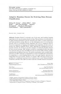
Fig. 1. Characteristics of the Electricity Dataset
We start by discussing an example of how researchers evaluate a data stream classifier using a real dataset representing a data stream. The Electricity dataset due to [15] is a popular benchmark for testing adaptive classifiers. It has been used in over 40 concept drift experiments5 , for instance, [10, 17, 6, 21]. The Electricity Dataset was collected from the Australian New South Wales Electricity Market. The dataset contains 45,312 instances which record electricity prices at 30 minute intervals. The class label identifies the change of the price (UP or DOWN) related to a moving average of the last 24 hours. The data is subject to concept drift due to changing consumption habits, unexpected events and seasonality. Two observations can be made about this dataset. Firstly, the data is not independently distributed over time, it has a temporal dependence. If the price goes UP now, it is more likely than by chance to go UP again, and vice versa. Secondly, the prior distribution of classes in this data stream is evolving. Figure 1 plots the class distribution of this dataset over a sliding window of 1000 instances and the autocorrelation function of the target label. We can see that data is heavily autocorrelated with very clear cyclical peaks at every 48 instances (24 hours), due to electricity consumption habits. Let us test two state-of-the-art data stream classifiers on this dataset. We test an incremental Naive Bayes classifier, and an incremental (streaming) decision tree learner. As a streaming decision tree, we use VFDT [16] with functional leaves, using Naive Bayes classifiers at the leaves. In addition, let us consider two naive baseline classifiers that do not use any input attributes and classify only using past label information: a moving majority class classifier (over a window of 1000) and a No-Change classifier that uses temporal dependence information by predicting that the next class label will be the same as the last seen class label. It can be compared to a naive weather forecasting rule: the weather tomorrow will be the same as today. We use prequential evaluation [11] over a sliding window of 1000 instances. The prequential error is computed over a stream of n instances as an accumulated loss L between the predictions yˆt and the true values yt : p0 =
n X t=1
5
Google scholar, 2013 March
L(ˆ yt , yt ).
100 Kappa Statistic, %
100 Accuracy, %
80 60 40 20 0
0
2 Time, instances No-Change Majority Class
80 60 40 20 0
4 4
·10
VFDT Naive Bayes
0
2 Time, instances No-Change Naive Bayes
4 ·104 VFDT
Fig. 2. Accuracy and Kappa Statistic on the Electricity Market Dataset
Since the class distribution is unbalanced, it is important to use a performance measure that takes class imbalance into account. We use the Kappa Statistic due to Cohen [7]. Other measures, such as, for instance, the Matthews correlation coefficient [19], could be used as well. The Kappa Statistic κ is defined as κ=
p0 − pc , 1 − pc
where p0 is the classifier’s prequential accuracy, and pc is the probability that a chance classifier - one that assigns the same number of examples to each class as the classifier under consideration—makes a correct prediction. If the tested classifier is always correct then κ = 1. If its predictions coincide with the correct ones as often as those of a chance classifier, then κ = 0. Figure 2 shows the evolving accuracy (left) of the two state-of-the-art stream classifiers and the two naive baselines, and the evolution of the Kappa Statistic (right). We see that the state-of-the-art classifiers seem to be performing very well if compared to the majority class baseline. Kappa Statistic results are good enough at least for the decision tree. Following the current evaluation practice for data stream classifiers we would recommend this classifier for this type of data. However, the No-Change classifier performs much better. Note that the No-Change classifier completely ignores the input attribute space, and uses nothing but the value of the previous class label. We retrospectively surveyed accuracies of 16 new stream classifiers reported in the literature that were tested on the Electricity dataset. Table 1 shows a list of the results reported using this dataset, sorted according to the reported accuracy. Only 6 out of 16 reported accuracies outperformed the No-Change classifier. This suggests that current evaluation practice needs to be revised. This paper makes a threefold contribution. First, in Section 2, we explain what is happening when data contains temporal dependence and why it is important to take into account when evaluating stream classifiers. Second, in Section 3, we propose a new measure to evaluate data stream classifiers taking into account possible temporal
Table 1. Accuracies of adaptive classifiers on the Electricity dataset reported in the literature. Algorithm name Accuracy (%) Reference DDM 89.6* [10] Learn++.CDS 88.5 [8] KNN-SPRT 88.0 [21] GRI 88.0 [22] FISH3 86.2 [23] EDDM-IB1 85.7 [1] No-Change classifier 85.3 ASHT 84.8 [6] bagADWIN 82.8 [6] DWM-NB 80.8 [17] Local detection 80.4 [9] Perceptron 79.1 [5] ADWIN 76.6 [2] Prop. method 76.1 [18] Cont. λ-perc. 74.1 [20] CALDS 72.5 [12] TA-SVM 68.9 [13] * tested on a subset
dependence. Third, in Section 5, we propose a generic wrapper classifier that enables conventional stream classifiers to take into account temporal dependence. In Section 4 we perform experimental analysis of the new measure. Section 6 concludes the study.
2
Why the Current Evaluation Procedures May Be Misleading
We have seen that a naive No-Change classifier can obtain very good results on the Kappa Statistic measure by using temporal information from the data. This is a surprising result since we would expect that a trivial classifier ignoring the input space entirely should perform worse than a well-trained intelligent classifier. Thus, we start by theoretically analyzing the conditions under which the No-Change classifier outperforms the majority class classifier. Next we discuss the limitations of the Kappa Statistic for measuring classification performance on data streams. Consider a binary classification problem with fixed prior probabilities of the classes P (c1 ) and P (c2 ). Without loss of generality assume P (c1 ) ≥ P (c2 ). The expected accuracy of the majority class classifier would be pmaj = P (c1 ). The expected accuracy of the No-Change classifier would be the probability that two labels in a row are the same pe = P (c1 )P (c1 |c1 ) + P (c2 )P (c2 |c2 ), where P (c1 |c1 ) is the probability of observing class c1 immediately after observing class c1 . Note that if data is distributed independently, then P (c1 |c1 ) = P (c1 ) and P (c2 |c2 ) = P (c2 ). Then the accuracy of the No-Change classifier is P (c1 )2 + P (c2 )2 . Using the fact that P (c1 ) + P (c2 ) = 1 it is easy to show that P (c1 ) ≥ P (c1 )2 + P (c2 )2 ,
that is pmaj ≥ pnc . The accuracies are equal only if P (c1 ) = P (c2 ), otherwise the majority classifier is more accurate. Thus, if data is distributed independently, then we can safely use the majority class classifier as a baseline. However, if data is not independently distributed, then, following similar arguments it can be shown that if P (c2 |c2 ) > 0.5 then P (c1 ) < P (c1 )P (c1 |c1 ) + P (c2 )P (c2 |c2 ). That is pmaj < pe , hence, the No-Change classifier will outperform the majority class classifier if the probability of seeing consecutive minority classes is larger than 0.5. This happens even in cases of equal prior probabilities of the classes. Similar arguments are valid in multi-class classification cases as well. If we observe the majority class, then the No-Change classifier predicts the majority class, the majority classifier predicts the same. They will have the same accuracy on the next data instance. If, however, we observe a minority class, then the majority classifier still predicts the majority class, but the No-Change classifier predicts a minority class. The NoChange strategy would be more accurate if the probability of observing two instances of that minority class in a row is larger than 1/k, where k is the number of classes. Table 2 presents characteristics of four popular stream classification datasets. Electricity and Airlines are available from the MOA6 repository, and KDD99 and Ozone are available from the UCI7 repository. Electricity and Airlines represent slightly imbalanced binary classification tasks, we see by comparing the prior and conditional probabilities that data is not distributed independently. Electricity consumption is expected to have temporal dependence. The Airlines dataset records delays of flights, it is likely that e.g. during a storm period many delays would happen in a row. We see that as expected, the No-Change classifier achieves higher accuracy than the majority classifier. The KDD99 cup intrusion detection dataset contains more than 20 classes, we report on only the three largest classes. The problem of temporal dependence is particularly evident here. Inspecting the raw dataset confirms that there are time periods of intrusions rather than single instances of intrusions, thus the data is not distributed independently over time. We observe that the No-Change classifier achieves nearly perfect accuracy. Finally, the Ozone dataset is also not independently distributed. If ozone levels rise, they do not diminish immediately, thus we have several ozone instances in a row. However, the dataset is also very highly imbalanced. We see that the conditional probability of the minority class (ozone) is higher than the prior, but not high enough to give advantage to the No-Change classifier over the majority classifier. This confirms our theoretical results. Thus, if we expect a data stream to contain temporal dependence, we need to make sure that any intelligent classifier is compared to the No-Change baseline in order to make meaningful conclusions about performance. Next we highlight issues with the prequential accuracy in such situations, and then move on to the Kappa Statistic. The main reason why the prequential accuracy may mislead is because it assumes that the data is distributed independently. If a data stream contains the same number of instances for each class, accuracy is the right measure 6 7
http://moa.cms.waikato.ac.nz/datasets/ http://archive.ics.uci.edu/ml/
Table 2. Characteristics of stream classification datasets P (c1 ) P (c2 ) P (c3 ) Majority acc. P (c1 |c1 ) P (c2 |c2 ) P (c3 |c3 ) No-Change acc. Electricity 0.58 0.42 0.58 0.87 0.83 0.85 Airlines 0.55 0.45 0.55 0.62 0.53 0.58 KDD99 0.60 0.18 0.17 0.60 0.99 0.99 0.99 0.99 Ozone 0.97 0.03 0.97 0.97 0.11 0.94 Dataset
to use, and will be sufficient to detect if a method is performing well or not. Here, a random classifier will have a 1/k accuracy for a k class problem. Assuming that the accuracy of our classifier is doing better than 1/k, we know that we are doing better than guessing the classes of the incoming instances at random. We see that when a data stream has temporal dependence, using only the Kappa Statistic for evaluating stream classifiers may be misleading. The reason is that when the stream has a temporal dependence, by using the Kappa Statistic we are comparing the performance of our classifier with a random classifier. Thus, we can view the Kappa Statistic as a normalized measure of the prequential accuracy p0 : p00 =
p0 − min p max p − min p
In the Kappa Statistic, we consider that max p = 1 and that min p = pc . This measure may be misleading because we assume that pc is giving us the accuracy of the baseline naive classifier. Recall that pc is the probability that a classifier that assigns the same number of examples to each class as the classifier under consideration, makes a correct prediction. However, we saw that the majority class classifier may not be the most accurate naive classifier when temporal dependence exists in the stream. NoChange may be a more accurate naive baseline, thus we need to take it into account within the evaluation measure.
3
New Evaluation for Stream Classifiers
In this section we present a new measure for evaluating classifiers. We start by more formally defining our problem. Consider a classifier h, a data set containing n examples and k classes, and a contingency table where cell Cij contains the number of examples for which h(x) = i and the class is j. If h(x) correctly predicts all the data, then all non-zero counts will appear along the diagonal. If h misclassifies some examples, then some off-diagonal elements will be non-zero. The classification accuracy is defined as Pk Cii . p0 = i=1 n
80
80
60 40 20 0
0
Kappa Plus Statistic, %
100 Kappa Statistic, %
Accuracy, %
100
60 40 20 0
2 4 Time, instances ·105
0
VFDT Maj. Class
No-Change N. Bayes
0
−200
−400
2 4 Time, instances ·105 No-Change N. Bayes
0
2 4 Time, instances ·105
VFDT
No-Change N. Bayes
VFDT
Fig. 3. Accuracy, κ and κ+ on the Forest Covertype dataset
Kappa Statistic, %
Accuracy, %
80
60 0
80 60 40 20 0
2 4 Time, instances ·105 No-Change Lev. Bagging
100 Kappa Plus Statistic, %
100
100
0
HAT
−100 −200 −300
2 4 Time, instances ·105 No-Change Lev. Bagging
0
0
2 4 Time, instances ·105
HAT
No-Change Lev. Bagging
Fig. 4. Accuracy, κ and κ+ on the Forest Covertype dataset
Let us define Pr[class is j] =
k X Cij i=1
n
, Pr[h(x) = i] =
k X Cij j=1
n
Then the accuracy of a random classifier is pc =
k X
(Pr[class is j] · Pr[h(x) = j])
j=1 k k k X X Cij X Cji = · n i=1 n j=1 i=1
! .
We can define pe as the following accuracy: pe =
k X j=1
2
(Pr[class is j]) =
k k X X Cij j=1
i=1
n
!2 .
.
HAT
Then the Kappa Statistic is κ=
p0 − pc . 1 − pc
Remember that if the classifier is always correct then κ = 1. If its predictions coincide with the correct ones as often as those of the chance classifier, then κ = 0. An interesting question is how exactly do we compute the relevant counts for the contingency table: using all examples seen so far is not useful in time-changing data streams. Gama et al. [11] propose to use a forgetting mechanism for estimating prequential accuracy: a sliding window of size w with the most recent observations. Note that, to calculate the statistic for a k class problem, we need to maintain only 2k + 1 estimators. We store the sum of all rows and columns in the confusion matrix (2k values) to compute pc , and we store the prequential accuracy p0 . Considering the presence of temporal dependencies in data streams we propose a new evaluation measure the Kappa Plus Statistic, defined as κ+ =
p0 − p0e 1 − p0e
where p0e is the accuracy of the No-Change classifier. κ+ takes values from 0 to 1. The interpretation is similar to that of κ. If the classifier is perfectly correct then κ+ = 1. If the classifier is achieving the same accuracy as the No-Change classifier, then κ+ = 0. Classifiers that outperform the No-Change classifier fall between 0 and 1. Sometimes it can happen that κ+ < 0, which means that the classifier is performing worse than the No-Change baseline. In fact, we can compute p0e as the probability that for all classes, the class of the new instance it+1 is equal to the last class seen in instance it . It is the sum for each class of the probability that the two instances in a row have the same class: p0e =
k X
(Pr[it+1 class is j and it class is j]) .
j=1
Two observations can be made about κ+ . First, when there is no temporal dependence, κ+ is closely related to κ since Pr[it+1 class is j and it class is j] = P r[it class is j]2 holds, and p0e = pe . It means that if there is no temporal dependence, then the probabilities of selecting a class will depend on the distributions of the classes, so does κ. Second, if classes are balanced and there is no temporal dependence, then κ+ is equal to κ and both are linearly related to the accuracy p0 : κ+ =
n 1 · p0 − . n−1 n−1
Therefore, using κ+ instead of κ, we will be able to detect misleading classifier performance for data that is dependently distributed. For highly imbalanced, but independently distributed data, the majority class classifier may beat the No-Change classifier.
κ+ and κ measures can be seen as orthogonal, since they measure different aspects of the performance. Hence, for a thorough evaluation we recommend measuring both. An interested practitioner can take a snapshot of a data stream and measure if there is a temporal dependency, e.g. by comparing the probabilities of observing the same labels in a row with the prior probabilities of the labels as reported in Table 2. However, even without checking whether there is a temporal dependency in the data a user can safely check both κ+ and κ. If there is no temporal dependency, both measures will give the same result. In case there is a temporal dependency a good classifier should score high in both measures.
4
Experimental Analysis of the New Measure
The goal of this experimental analysis is to compare the informativeness of κ and κ+ in evaluating stream classifiers. These experiments are meant to be merely a proof of concept, therefore we restrict the analysis to two data stream benchmark datasets. The first, the Electricity dataset was discussed in the introduction. The second, Forest Covertype, contains the forest cover type for 30 × 30 meter cells obtained from US Forest Service (USFS) Region 2 Resource Information System (RIS) data. It contains 581, 012 instances and 54 attributes, and has been used in several papers on data stream classification. We run all experiments using the MOA software framework [3] that contains implementations of several state-of-the-art classifiers and evaluation methods and allows for easy reproducibility. The proposed κ+ is not base classifier specific, hence we do not aim at exploring a wide range of classifiers. We select several representative data stream classifiers for experimental illustration. Figure 3 shows accuracy of the three classifiers Naive Bayes, VFDT and No-Change using the prequential evaluation of a sliding window of 1000 instances, κ results and results for the new κ+ . We observe similar results to the Electricity Market dataset, and that for the No-Change classifier κ+ is zero, and for Naive Bayes and VFDT, κ+ is negative. We also test two more powerful data stream classifiers: – Hoeffding Adaptive Tree (HAT): which extends VFDT to cope with concept drift. [3]. – Leveraging Bagging: an adaptive ensemble that uses 10 VFDT decision trees [4]. For the Forest CoverType dataset, Figure 4 shows accuracy of the three classifiers HAT, Leveraging Bagging and No-Change using a prequential evaluation of a sliding window of 1000 instances. It also shows κ results and the new κ+ results. We see how these classifiers improve the results over the previous classifiers, but still have negative κ+ results, meaning that the No-Change classifier is still providing better results. Finally, we test the two more powerful stream classifiers on the Electricity Market dataset. Figure 5 shows accuracy, κ and κ+ for the three classifiers HAT, Leveraging Bagging and No-Change . κ+ is positive for a long period of time, but still contains some negative results.
100
80
60 0
2 4 Time, instances ·104 No-Change Lev. Bagging
HAT
100 Kappa Plus Statistic, %
Kappa Statistic, %
Accuracy, %
100
80 60 40 20 0
0
2 4 Time, instances ·104 No-Change Lev. Bagging
0 −100 −200 −300
HAT
0
2 4 Time, instances ·104 No-Change Lev. Bagging
HAT
Fig. 5. Accuracy, κ and κ+ on the Electricity Market dataset
Our experimental analysis indicates that using the new κ+ measure, we can easily detect when a classifier is doing worse than the simple No-Change strategy, by simply observing if negative values of this measure exist.
5
S WT: Temporally Augmented Classifier
Having identified the importance of temporal dependence in data stream classification we now propose a generic wrapper that can be used to wrap state-of-the-art classifiers so that temporal dependence is taken into account when training an intelligent model. We propose S WT, a simple meta strategy that builds meta instances by augmenting the original input attributes with the values of recent class labels from the past (in a sliding window). Any existing incremental data-stream classifier can be used as a base classifier with this strategy. The prediction becomes a function of the original input attributes and the recent class labels P r[class is c] ≡ h(xt , ct−` , . . . , ct−1 ) for the t-th test instance, where ` is the size of the sliding window over the most recent true labels. The larger `, the longer temporal dependence is considered. h can be any of the classifiers we mentioned (e.g., HAT or Leveraging Bagging). It is important to note that such a classifier relies on immediate arrival of the previous label after the prediction is casted. This assumption may be violated in real-world applications, i.e. true labels may arrive with a delay. In such a case it is still possible to use the proposed classifier with the true labels from more distant past. The utility of this approach will depend on the strength of the temporal correlation in the data. We test this wrapper classifier experimentally using HAT and VFDT as the internal stream classifiers. In this proof of concept study we report experimental results using ` = 1. Our goal is to compare the performance of an intelligent S WT, with that of the baseline No-Change classifier. Both strategies take into account temporal dependence. However, S WT, does so in an intelligent way considering it alongside a set of input attributes.
100
80
80
40 20 0
0
20 0
S WT VFDT
100
100
80
80
60 40 20 0
0
2 4 Time, instances ·104
No-Change S WT Lev. Bagging
S WT HAT
2 4 Time, instances ·104 No-Change S WT N. Bayes
Kappa Statistic, %
Accuracy, %
40
0
2 4 Time, instances ·104 No-Change S WT N. Bayes
60
−100 −200 −300
S WT VFDT
0
2 4 Time, instances ·104 No-Change S WT N. Bayes
S WT VFDT
100
60 40 20 0
0
Kappa Plus Statistic, %
60
100 Kappa Plus Statistic, %
100 Kappa Statistic, %
Accuracy, %
Figure 6 shows the S WT strategy applied to VFDT, Naive Bayes, Hoeffding Adaptive Tree, and Leveraging Bagging for the Electricity dataset. The results for the Forest Cover dataset are displayed in Figure 7. As a summary, Figure 8 (left and center) shows κ+ on the Electricity and Forest Cover datasets. We see a positive κ+ which means that the prediction is meaningful taking into account the temporal dependency in the data. Additional experiments reported in Figures 9, 10, 11 confirm that the results are stable under varying size of the sliding window (to ` > 1) and varying feature space (i.e., xt−` , . . . , xt−1 ). More importantly, we see a substantial improvement as compared to the state-of-the-art stream classifiers (Figures 3, 4, 5) that do not use the temporal dependency information.
0
2 4 Time, instances ·104
No-Change S WT Lev. Bagging
S WT HAT
0 −100 −200 −300
0
2 4 Time, instances ·104
No-Change S WT Lev. Bagging
Fig. 6. Accuracy, κ and κ+ on the Electricity Market dataset for the S WT classifiers
S WT HAT
80
80
40 20 0
0
40 20 0
2 4 Time, instances ·105 No-Change S WT N. Bayes
0
S WT VFDT
100
100
80
80
60 40 20 0
0
No-Change S WT Lev. Bagging
20
S WT HAT
0
2 4 Time, instances ·105 No-Change S WT N. Bayes
S WT VFDT
100
40
0
−1,000
S WT VFDT
60
2 4 Time, instances ·105
−500
2 4 Time, instances ·105 No-Change S WT N. Bayes
Kappa Statistic, %
Accuracy, %
60
Kappa Plus Statistic, %
60
0 Kappa Plus Statistic, %
100 Kappa Statistic, %
Accuracy, %
100
0
2 4 Time, instances ·105
No-Change S WT Lev. Bagging
0 −100 −200 −300
S WT HAT
0
2 4 Time, instances ·105
No-Change S WT Lev. Bagging
S WT HAT
Fig. 7. Accuracy, κ and κ+ on the Forest Covertype dataset for the S WT classifiers
Electricity dataset
0 −50
0
2 4 Time, instances ·104 No-Change S WT HAT
S WT VFDT
100 Accuracy of S WT, %
Kappa Plus Statistic, %
Kappa Plus Statistic, %
100
50
−100
Electricity dataset
Forest Cover dataset
100
50 0 −50 −100
0
2 4 Time, instances ·105 No-Change S WT HAT
S WT VFDT
90
80
70 70
80 90 100 Accuracy of No-Change , % S WT VFDT S WT HAT baseline
Fig. 8. κ+ and accuracy of the S WT VFDT, S WT HAT, and No-Change classifiers
100
1.8
60 40
1.4 1.2
20 0
1.6
Memory (Kb)
Time (sec.)
80 400
200
1 0
20 40 ` size of the sliding window
Accuracy Kappa Plus Statistic
0
Kappa Statistic
20 40 ` size of the sliding window
0
20 40 ` size of the sliding window Memory
Time
Fig. 9. Accuracy, κ, κ+ , time and memory of a VFDT on the Electricity Market dataset for the S WT classifiers varying the size of the sliding window parameter `
100 200 Time (sec.)
60 40
Memory (Kb)
2.5
80
2
100
20 0
0 0
20 40 ` size of the sliding window
Accuracy Kappa Plus Statistic
0
0
20 40 ` size of the sliding window
20 40 ` size of the sliding window Memory
Time
Kappa Statistic
Fig. 10. Accuracy, κ, κ+ , time and memory of a Hoeffding Adaptive Tree on the Electricity Market dataset for the S WT classifiers varying the ` size of the sliding window parameter
6,000
100 20
60 40
15
10
20 0
Memory (Kb)
Time (sec.)
80
0
20 40 ` size of the sliding window
Accuracy Kappa Plus Statistic
Kappa Statistic
0
20 40 ` size of the sliding window Time
4,000
2,000
0
20 40 ` size of the sliding window Memory
Fig. 11. Accuracy, κ, κ+ , time and memory of a Leveraging Bagging on the Electricity Market dataset for the S WT classifiers varying the ` size of the sliding window parameter
6
Conclusion
As researchers, we may have not considered temporal dependence in data stream mining seriously enough when evaluating stream classifiers. In this paper we explain why it is important, and we propose a new evaluation measure to consider it. We encourage the use of the No-Change classifier as a baseline, and compare classification accuracy against it. We emphasize, that a good stream classifier should score well on both: the existing κ and the new κ+ . In addition, we propose a wrapper classifier S WT, that allows to take into account temporal dependence in an intelligent way and, reusing existing classifiers outperforms the No-Change classifier. Our main goal with this proof of concept study is to highlight this problem of evaluation, so that researchers in the future will be able to build better new classifiers taking into account temporal dependencies of streams. This study opens several directions for future research. The wrapper classifier S WTis very basic and intended as a proof of concept. One can consider more advanced (e.g. non-linear) incorporation of the temporal information into data stream classification. Ideas from time series analysis could be adapted. Performance and evaluation of change detection algorithms on temporally dependent data streams present another interesting direction. We have observed ([24]) that under temporal dependence detecting a lot of false positives actually leads to better prediction accuracy than a correct detection. This calls for an urgent further investigation. ˇ Acknowledgments. I. Zliobait˙ e’s research has been supported by the Academy of Finland grant 118653 (ALGODAN).
References 1. M. Baena-Garcia, J. del Campo-Avila, R. Fidalgo, A. Bifet, R. Gavalda, and R. MoralesBueno. Early drift detection method. In Proc. of the 4th ECMLPKDD Int. Workshop on Knowledge Discovery from Data Streams, pages 77–86, 2006. 2. A. Bifet and R. Gavalda. Learning from time-changing data with adaptive windowing. In Proc. of the 7th SIAM Int. Conf. on Data Mining, SDM, 2007. 3. A. Bifet, G. Holmes, R. Kirkby, and B. Pfahringer. MOA: Massive online analysis. J. of Mach. Learn. Res., 11:1601–1604, 2010. 4. A. Bifet, G. Holmes, and B. Pfahringer. Leveraging bagging for evolving data streams. In Proc. of the 2010 European conf. on Machine learning and knowledge discovery in databases, ECMLPKDD, pages 135–150, 2010. 5. A. Bifet, G. Holmes, B. Pfahringer, and E. Frank. Fast perceptron decision tree learning from evolving data streams. In Proc of the 14th Pacific-Asia Conf. on Knowledge Discovery and Data Mining, PAKDD, pages 299 – 310, 2010. 6. A. Bifet, G. Holmes, B. Pfahringer, R. Kirkby, and R. Gavald`a. New ensemble methods for evolving data streams. In Proc. of the 15th ACM SIGKDD int. conf. on Knowledge discovery and data mining, KDD, pages 139–148, 2009. 7. J. Cohen. A coefficient of agreement for nominal scales. Educational and Psychological Measurement, 20(1):37–46, 1960. 8. G. Ditzler and R. Polikar. Incremental learning of concept drift from streaming imbalanced data. IEEE Transactions on Knowledge and Data Engineering, 2013.
9. J. Gama and G. Castillo. Learning with local drift detection. In Proc. of the 2nd int. conf. on Advanced Data Mining and Applications, ADMA, pages 42–55, 2006. 10. J. Gama, P. Medas, G. Castillo, and P. Rodrigues. Learning with drift detection. In Proc. of the 7th Brazilian Symp. on Artificial Intelligence, SBIA, pages 286–295, 2004. 11. J. Gama, R. Sebasti˜ao, and P. Rodrigues. On evaluating stream learning algorithms. Machine Learning, 90(3):317–346, 2013. 12. J. Gomes, E. Menasalvas, and P. Sousa. CALDS: context-aware learning from data streams. In Proc. of the 1st Int. Workshop on Novel Data Stream Pattern Mining Techniques, StreamKDD, pages 16–24, 2010. 13. G. Grinblat, L. Uzal, H. Ceccatto, and P. Granitto. Solving nonstationary classification problems with coupled support vector machines. IEEE Transactions on Neural Networks, 22(1):37–51, 2011. 14. D. Hand. Classifier technology and the illusion of progress. Statist. Sc., 21(1):1–14, 2006. 15. M. Harries. SPLICE-2 comparative evaluation: Electricity pricing. Tech. report, University of New South Wales, 1999. 16. G. Hulten, L. Spencer, and P. Domingos. Mining time-changing data streams. In Proc. of the 7th ACM SIGKDD int. conf. on Knowl. disc. and data mining, KDD, pages 97–106, 2001. 17. J. Kolter and M. Maloof. Dynamic weighted majority: An ensemble method for drifting concepts. J. of Mach. Learn. Res., 8:2755–2790, 2007. 18. D. Martinez-Rego, B. Perez-Sanchez, O. Fontenla-Romero, and A. Alonso-Betanzos. A robust incremental learning method for non-stationary environments. Neurocomput., 74(11):1800–1808, 2011. 19. B. Matthews. Comparison of the predicted and observed secondary structure of T4 phage lysozyme. Biochimica et biophysica acta, 405(2):442–451, 1975. 20. N. Pavlidis, D. Tasoulis, N. Adams, and D. Hand. Lambda-perceptron: An adaptive classifier for data streams. Pattern Recogn., 44(1):78–96, 2011. 21. G. Ross, N. Adams, D. Tasoulis, and D. Hand. Exponentially weighted moving average charts for detecting concept drift. Pattern Recogn. Lett, 33:191–198, 2012. 22. J. Tomczak and A. Gonczarek. Decision rules extraction from data stream in the presence of changing context for diabetes treatment. Knowl. Inf. Syst., 34(3):521–546, 2013. 23. I. Zliobaite. Combining similarity in time and space for training set formation under concept drift. Intell. Data Anal., 15(4):589–611, 2011. 24. I. Zliobaite. How good is the electricity benchmark for evaluating concept drift adaptation. CoRR, abs/1301.3524, 2013.