Amirkabir University of Technology (Tehran Polytechnic)
Amirkabir International Jounrnal of Science & Research
Modeling, Identification, Simulation and Control (AIJ-MISC) Vol. 48, No. 2, Fall 2016, pp. 75-91
Potentials of Evolving Linear Models in Tracking Control Design for Nonlinear Variable Structure Systems A. Kalhor1,*, N. Hojjatzadeh2, A. Golgouneh3 1- Assistant Professor, School of Electrical and Computer Engineering, University of Tehran 2- M.Sc. Student, Faculty of New Sciences and Technologies, University of Tehran 3- M.Sc. Student, Faculty of New Sciences and Technologies, University of Tehran (Received 15 May 2016, Accepted 3 September 2016)
ABSTRACT Evolving models have found applications in many real world systems. In this paper, potentials of the Evolving Linear Models (ELMs) in tracking control design for nonlinear variable structure systems are introduced. At first, an ELM is introduced as a dynamic single input, single output (SISO) linear model whose parameters as well as dynamic orders of input and output signals can change through the time. Then, the potential of ELMs in modeling nonlinear time-varying SISO systems is explained. Next, the potential of the ELMs in tracking control of a minimum phase nonlinear time-varying SISO system is introduced. To this end, two tracking control strategies are proposed, respectively for (a) when the ELM is known perfectly and (b) when the ELM model has uncertainties but dynamic orders of the input and output signals are fixed. The methodology and superiority of the proposed tracking control systems are shown via some illustrative examples: speed control in a DC motor and link position control in a flexible joint robot.
KEYWORDS: Evolving Linear Model, Nonlinear Time-Varying Systems, Tracking Control System
Please cite this article using: Kalhor, A., Hojjatzadeh, N., and Golgouneh, A., 2016. “Potentials of Evolving Linear Models in Tracking Control Design for Nonlinear Variable Structure Systems”. Amirkabir International Journal of Modeling, Identification, Simulation and Control, 48(2), pp. 75–91. DOI: 10.22060/miscj.2016.829 URL: http://miscj.aut.ac.ir/article_829.html * Corresponding Author, Email:
[email protected] AIJ - Modeling, Identification, Simulation and Control, Vol 48, No. 2, Fall 2016
75
Potentials of Evolving Linear Models in Tracking Control Design for Nonlinear Variable Structure Systems
1- INTRODUCTION
A. MOTIVATION AND RELATED WORKS
Nonlinearity and structural variability cause significant challenges in control design, particularly when the system is not affine or there are uncertainties. Robust control and adaptive control methods have been introduced and developed for such systems. Whereas robust control guarantees the stability and performance of the system under bounded uncertainties, adaptive control satisfies the required performance and stability by posing adaptation rules for the controller with regard to the new condition of the system. Among known robust control strategies, H-infinity, μ-synthesis and sliding mode are more popular and applicable. Considering unstructured uncertainty in a control system, H-infinity based methods are used to minimize the closed loop impact of perturbation [1,2] and in recent years, new aspects of the H-infinity are studied [3,4]. μ-synthesis based methods unlike H-infinity are used to design robust control against certain structured uncertainties [5,6]. Sliding mode control is a variable structure control method providing a systematic approach to the problem of maintaining stability in the face of modeling uncertainty [7,8]. This approach has been also used and developed in many nonlinear control systems [9-11]. A wide range of methods have been introduced in the literature of adaptive control systems. Adaptive pole placement, different self-tuning regulators and iterative learning control are straightforward techniques using direct or indirect approaches to provide stability and performance in the system [1214]. However, they are suggested principally for linear systems. Model Reference Adaptive Controllers often suggest direct solutions for adaptive control of continuous time systems based on a reference model. Regarding the structure of the system, the reference model can be chosen linear or nonlinear as well [15-17]. Gain scheduling based methods offer a set of control strategies corresponding to different operating regimes of the system prepared as a table [18,19]. Such methods are also developed for nonlinear and also time-varying systems. Also, for nonlinear systems, adaptive control systems such as self-oscillating adaptive systems [20,21], variable structure system [22,23] and duality controllers [24,25], have been proposed. On the other hand, during last decade, evolving
76
fuzzy and neuro-fuzzy models have been developed in modeling nonlinearity and time-varying structures. In an evolving model, the structure can evolve through the time based on observing samples of input and output signals. The structure of a nonlinear evolving model often can be described as an interpolated of locally linear models constructed from simple if-then fuzzy rules. There are two particularly influential works in this area of research [26,27]. Kasabov proposes an adaptive online learning algorithm as a dynamic evolving neural–fuzzy inference system (DENFIS). In this algorithm, fuzzy inference rules are created by using maximum distance clustering, which is utilized in partitioning of input space. Angelov and Filev introduce an online identification approach for the Takagi Sugeno (TS) model, where evolving clustering method along with a concept of potential is used to define the antecedent parts of the rules. This approach has been modified in [28] and [29]. In [30], to evolve a specific form of TS Fuzzy Model, Lughofer suggests to use a modified version of vector quantization for new rule generation. Although evolving nonlinear systems have been developed successfully in simulation, approximation, classification and prediction, they are not straightforward basis for analyzing and designing control systems, In recent years, by the author and its cooperators, there is a tendency toward using and developing Evolving Linear Models (ELMs) [31,32]. An ELM can adapt and follow the variations of the nonlinear and time-varying system with agility [33]. Moreover, it seems ELMs can fulfill facilities in control, analyze and design due to their linear forms.
B. OUR CONTRIBUTIONS
In this paper, some potentials of ELMs in tracking control of nonlinear variable structure systems are introduced. It is shown that if nonlinear models could be represented as ELMs, two significant challenges in tracking control systems will be solved. At first, the nonlinear systems do not have essentially an affine structure with regard to the input signal. This avoids using some given classic solutions like feedback linearization or sliding mode control [8] by which a stable differential equation of error is satisfied. ELM represents the system in an affine form which allows one to design a tracking control system easily for nonlinear non-affine systems. Also, when the dynamic order of a nonlinear system changes, computing its impulse effects is not straightforward and this causes
AIJ - Modeling, Identification, Simulation and Control, Vol. 48, No. 2, Fall 2016
A. Kalhor, N. Hojjatzadeh, A. Golgouneh
that one cannot solve the tracking control problem even when a general solution like lyapunov method is existed. Using ELMs allows the input signal to be computed in order that the tracking control system in switching time remains stable. Also, it is proved that using ELMs allows us to use Sliding Mode Control (SMC) for when the system has some inherent uncertainties or the linearization of the nonlinear system causes some bounded uncertainties. The rest of the paper is organized as follows: in section II, ELMs are introduced, then in section III the potential of ELM in modeling nonlinear models is explained and in section IV, the potential of ELM in tracking control systems are explained. In section V, the conclusion remarks are given.
2- EVOLVING LINEAR MODELS
An evolving linear model (ELM), in continuous time domain, is defined as a linear differential equation between input signal u(t) ϵ R and output signal y(t) ϵ R of a SISO system:
(1) where nt and mt, respectively denote dynamic orders of output and input signals which are bounded to nmax and mmax. Also, ai(t) ϵ R , bj(t) ϵ R denote respectively linear parameters for ith and jth derivatives of y(t) and u(t), and c(t) ϵ R denotes the bias parameter. In this paper, x[l](t) denotes the lth derivative of the signal x(t). As it is seen in (1), linear parameters as well as dynamic orders of exogenous input and output can change through the time. Assumption 1: In an ELM, the dynamic orders of input and output signals can change only at finite instants named as evolving instants (EIs). The set of EIs for the introduced ELM in (1) is defined as follows:
(3) Fig. 1 shows a diagram representing ELM model as switching LTI models. The above representation shows that ELMs is more capable of modeling nonlinearity than dynamic local linear models, such as ANFIS in [34], LOLIMOT in [35] and TS-SAMC in [36]. This is because, in such models the number of Local Linear Models (LLMs) is restricted and the output is defined as an interpolation of LLMs but in an ELM at each working point there is an independent LLM and the number of LLMs is not restricted; moreover, unlike most of the locally linear neuro-fuzzy models, in an ELM the dynamic order of the input or output can change at EIs.
3- POTENTIAL OF ELM IN MODELING NONLINEAR MODELS
A. TIME-VARYING NONLINEAR MODEL WITH TIME-VARYING DYNAMIC ORDER
Consider following input-output representation of a time-varying nonlinear model: (4) where F(nt,mt) denotes a time-varying nonlinear function of the input and output signals and their derivatives; nt and mt, respectively denote dynamic orders of the output and input signals at time t and their possible maximum values are nmax and mmax. Actually, the structure of a nonlinear dynamic model
(2) In another representation, an ELM can be supposed as a model which switches at each instancet to a new LTI model whose parameters and dynamic orders are fixed. Fig. 1. An evolving linear model is represented as switching LTI models
AIJ - Modeling, Identification, Simulation and Control, Vol. 48, No. 2, Fall 2016
77
Potentials of Evolving Linear Models in Tracking Control Design for Nonlinear Variable Structure Systems
may change through the time due to internal physical variations, erosions, delays and environmental factors. Assumption 2: For the function F(nt,mt)–similar to the considered assumption for ELMs–the dynamic order of the input and output signal: nt and mt can change just at finite instancets, i.e. EIs. Consider that the set A={σ1,σ2,…,σF} denotes EIs for the F(nt,mt)). Assumption 3: The function F(nt,mt)) and its variables are continuously differentiable except at its EIs.
C. POTENTIAL OF ELM IN MODELING CONTROL SYSTEMS
Consider T as sampling period of the input and output of the system. Considering variation variables: δy[i](t)=y[i](t)‑y[i](t‑T), δu[j](t)=u[j](t)‑u[j](t‑T) and δt=T, the Jacobian of the given nonlinear dynamic function in (4), for ∀tϵ(R‑A), can be stated as follows:
(5) where γ(t,T) denotes all high order terms in Taylor series; one can suppose that if for at least one coefficient of the input variations was not zero, γ(t,T) is negligible for small enough sampling period T. Here, we assume γ(t,T) and its derivatives are restricted. The above model in (5) can be also rewritten as follows:
stated as an ELM: (7) Definition 1: Corresponding to each time-varying nonlinear SISO system represented in (4), if Assumption 2 and Assumption 3 are satisfied, an ELM can be defined as (6) and (7).
4- POTENTIAL OF ELM IN TRACKING CONTROL SYSTEMS
In this section, for tracking control system of an ELM, two different control strategies are proposed, respectively for two different states: (a) the ELM is known perfectly and (b) the ELM is known but with some uncertainties. In the first state, it is assumed that the dynamic order can change through the time but in the second state, for the sake of simplicity, it is assumed the dynamic orders for the input and output signals are fixed through the time.
A. CONTROL STRATEGY FOR A KNOWN ELM
In this section, it is supposed that the ELM in (7) is perfectly known and there is no uncertainty in the model. Considering some assumptions and using a control strategy, it is aimed that the output of the system asymptotically converges to the reference signal. Assumption 4: For the ELM in (7), ∀t:∃ jϵ{0,1,… ,mmax}|bj(t)≠0. Assumption 5: The zero dynamic in (7) m0
∑b (t )u [ ] (t ) = α (t ) is stable for any bounded signal (6)
j =0
j
j
α(t). Assumption 6: The reference signal, yr(t), is real, bounded and continuously differentiable for all t >0. Theorem 1: Considering Assumptions 4-6 and applying the computed signal control from (8) to the system (4), the output y(t), will converge to yr(t)+π(t):
Here, the Jacobian of the nonlinear model at EIs: σh, h=1,2,…,F is defined as the same Jacobian for {t|t→σh+}. Accordingly, we can define the Jacobian for all over the time. Considering ai(t)=(∂F(nt,mt) / (∂uj(t)), bj(t)=(∂F(nt,mt)) / (∂uj(t)), c(t)=r(t) and respecting to (1), the considered nonlinear function in (4) can be
78
AIJ - Modeling, Identification, Simulation and Control, Vol. 48, No. 2, Fall 2016
(8)
A. Kalhor, N. Hojjatzadeh, A. Golgouneh
equation:
(13)
where the roots of the characteristic function: snma x+d snmax‑1+d snmax‑2+...+d nmax=0 are in the left part of 1 2 the complex plane s=σ+jω and σt denotes the last evolving instant before t.
In fact, by computing the control signal from above equation the initially considered EBE will be satisfied. The response of the EBE is the sum of the response to initial condition and the response to the input signal. We can discount response to the initial condition because it decays through the time. However, we can compute the steady response by applying the Laplace Transform to the EBE: (14)
(9)
Now by applying the inverse of the Laplace Transform, we get: where δ(.) denotes the Dirak delta function. Proof: Assume the following error differential equation:
(10)
We call the above differential equation Error Based Equation (EBE). Now, we compute the signal control which satisfies EBE. Regarding initial conditions for EBE at σt, by nmax‑nt times integral of the EBE, one can get the following equation:
(15) Accordingly, the e(t) will converge to π(t,T) or y(t) will converge to yr(t)+π(t,T). Here, two important notes about the Theorem 1 are stated: 1) If T converges to zero, γ(t,T), its derivatives and accordingly π(t,T) converges to zero and y(t) will follow yr(t), asymptotically. 2) The signal control u(t) can be computed easily by solving the non-homogenous time-varying linear differential equation in (7) [37]. This differential equation must be solved separately for each interval in which the dynamic order mt is fixed; also, when mt changes, the given initial conditions are considered.
1) ILLUSTRATIVE EXAMPLE (11)
As it is understood, the considered Dirac delta functions in EBE eliminate the effects of initial conditions from γ(t,T) and its derivatives. Now, by considering e[nt](t)=y[nt](t)‑yr[nt](t) we have: (12) Putting the ELM in (7) in the left hand of the above equation, we get the following differential
The Dynamics of a DC motor is stated as the following state model: (16) where x1 is the armature current, x2 is the motor speed , u is the field current and θ1 to θ5 are positive constants [8,38]. Assume the domain of operations will be restricted to regimes that the system is minimum phase. It is desired to design a controller based on
AIJ - Modeling, Identification, Simulation and Control, Vol. 48, No. 2, Fall 2016
79
Potentials of Evolving Linear Models in Tracking Control Design for Nonlinear Variable Structure Systems
Theorem 1 such that the output y asymptotically tracks the reference signal yr(t)=2+0.5sin(2t). For this reason, three following cases are considered: Case 1: T=0.001 seconds, θ1=θ2=θ4=θ5=1 and θ3=5 for t≥0. Case 2: T=0.1 seconds, θ1=θ2=θ4=θ5=1 and θ3=5 for t≥0. Case 3: T=0.001 seconds: - θ1=θ2=θ4=θ5=1 and θ3=5 : 0