Power Transmission Control Using Distributed Max-Flow A. Armbruster M. Gosnell B. McMillin M. Crow {aearmbru, mrghx4, ff}@umr.edu
[email protected] Department of Computer Science School of Materials, Energy, and Earth Resources Intelligent Systems Center University of Missouri–Rolla, Rolla, MO 65409-0350
Abstract— Existing maximum flow algorithms use one processor for all calculations or one processor per vertex in a graph to calculate the maximum possible flow through a graph’s vertices. This is not suitable for practical implementation. We extend the max-flow work of Goldberg and Tarjan to a distributed algorithm to calculate maximum flow where the number of processors is less than the number of vertices in a graph. Our algorithm is applied to maximizing electrical flow within a power network where the power grid is modeled as a graph. Error detection measures are included to detect problems in a simulated power network. We show that our algorithm is successful in executing quickly enough to prevent catastrophic power outages. Index Terms— Fault Injection, FT Algorithms, FT Communication, maximum flow, power system.
S
(100,100)
(50,50) E (22,22)
(28,28)
(50,50) D
(15,15)
(8,8) B
A (17,17)
(10,10)
(20,20) (3,3)
(40,40) C
I. I NTRODUCTION A maximum flow (max-flow) algorithm calculates the maximum flow possible between two given vertices through a connected graph. Although sequential and distributed algorithms exist for calculating max-flow, they are not practical for all applications. Existing max-flow algorithms use either one processor or one processor per vertex in a graph. In a realworld system, such as power flow control, many vertices will be computed by a single processor. We present a distributed algorithm to calculate the maximum flow where the number of processors is less than the number of vertices in the graph. Our algorithm is applied to electrical flow in a power network where the power grid is modeled as a graph. Fault tolerance measures are included in our application to govern problems in the simulated power network. Section II gives a background of maximum flow within a graph and its relationship to a power network. Our distributed maximum flow algorithm is presented in Section III. Error detection based on assertion checking is used to produce a fail-stop system for simulations on power systems. Section IV presents timing and error detection results from applying the algorithm to a power network simulation. A conclusion and future work follow in Sections V and VI, respectively. II. BACKGROUND A. Power Transmission as a Graph The power transmission grid can be modeled as a directed graph with power flowing from generators (sources) to loads This research supported in part by NSF IGERT grant DGE-9972752, NSF MRI grant CNS-0420869, and in part by the UMR Intelligent Systems Center.
(10,10)
(30,30)
t
Fig. 1. Power network shown as a directed flow graph with virtual vertices s and t. Edges are labeled with (flow, capacity). The capacity over all edges is fully utilized.
(sinks). Given a graph G′ (V ′ , E ′ ) where the set of vertices, V ′ , corresponds to the buses of the power network, the power flowing between vertices vi , vj ∈ V ′ is represented by an edge (vi , vj ) ∈ E ′ . For each vertex v ∈ V ′ , power in must equal power out. Generators, however, can be modeled as outputting power without any input and loads can be modeled as power in with no power out. This can be modeled as a flow problem by adding to the graph a virtual source, s, that connects to all the generators, and a virtual sink, t which connects to all loads [1]. The virtual source can supply infinite power, but its outward arcs are limited by the generator capacities. The virtual sink can potentially consume an infinite amount of power flow, but is constrained by the inward arcs representing loads. The resultant graph, G(V, E), is shown in Fig. 1. A power network G′ (V ′ , E ′ ) corresponding to the graph from Fig. 1 is shown in Fig. 2. The power network example shows generators at locations A and B which were supplied by s in Fig. 1. The arrows not connected to another power bus, or vertex, represent the edges to the virtual sink. It can be seen from Fig. 2 that the power in each edge of G′ corresponds to
E
III. M AX -F LOW
28 100
50
A
50
B
~
15
40
A. Sequential Max-Flow
22
17
D
3
~
8 20 10
10
C 30
Fig. 2. Example power system network with generators of 100 at A and 50 B and loads of 40, 50, 20, 30, and 10.
the maximum flow in each edge of G. B. Controlling Power Flow Cascading failures are the most severe form of failure that can occur in a power system. A cascading failure occurs when the loss of one line leads to the loss of another until the transmission grid can no longer sustain the power flow. Cascading failures have occurred in the United States in the 1960’s, 1970’s, and 2003. One reason for cascading failures is that present control of the transmission grid limits power service providers to selecting which lines are available, not how much power flows through them. When a power line is lost, remaining power redistributes throughout the grid according to the laws of physics. Since natural power flow is not determined by the capacity of the line, a line can be overloaded even though there is enough remaining capacity in the grid to transfer the power. To mitigate overloads, power companies either manually trip off a line when too much power is flowing through or redistribute generation. To use the other transmission lines that can handle the flow, power electronic devices need to be used to change properties of the lines so that power will choose to use the capacity of all lines. Flexible AC Transmission System (FACTS) devices can change power line properties and control the amount of flow on a line, preventing cascading failures due to line loss [2]. However, determining and coordinating FACTS devices is crucial to finding settings that will avoid cascading failures. A natural approach to calculate flow and determine FACTS settings is to model the power flow as a maximum flow problem as first reported in [3]. Using techniques from Section II-A, one can model the power network as a graph with vertex set V . Each FACTS device, Pi ∈ P contains power electronics and an embedded computer and computes settings for a subset of vertices Vpi using the state of the power system as a weighted graph of line flows. The state can be obtained through the techniques described in [4]. A distributed maxflow algorithm can then be used to determine settings to force the flow on the lines where FACTS devices are located. In the worst case, if the power network can no longer satisfy the load, max-flow can also shed load.
The sequential max-flow algorithm was developed in 1955 to calculate commodity flows in a graph. Many improvements followed, leading to the push and relabel method pioneered by Goldberg [5] that was further refined with Tarjan [6]. The push and relabel algorithm builds a ladder with vertices on various rungs. The flow can only pass from one vertex to a vertex a level below it [6]. B. Distributed Max-Flow In addition to the many sequential max-flow algorithms, several parallel or distributed max-flow algorithms have been developed [6]–[8]. Three solutions were presented by Goldberg and Tarjan: a parallel solution using a PRAM model, a synchronous distributed model, and an asynchronous distributed algorithm that requires one processor per vertex [6]. The asynchronous variant works by sending messages listed in Definition 3.1, which constitute the message sets in Definition 3.2. When flow is pushed from one graph vertex to another, a message PFm is sent. Each vertex maintains a distance variable that is the distance from the sink, t. The receiving vertex first checks the distance in the message to verify that the message can be accepted. If the distance sent is one more than the current distance, an accept message AFm is returned; otherwise, a reject message RFm is sent as the reply. A distance message, Distm, is sent to every neighboring vertex every time the distance at a vertex is updated. Although there are several distributed max-flow algorithms, for example the Goldberg-Tarjan asynchronous algorithm, none of them address the problem of executing where a single processor handles multiple vertices. Definition 3.1: Max-Flow Message Types Cm: The message currently being processed. PFm: A message attempting to push flow to a neighboring vertex. AFm: A message replying to a PFm indicating the requested flow is accepted. RFm: A message replying to a PFm indicating the requested flow cannot be accepted. Distm: A distance message indicating an update to a nodes distance. MFm: A max-flow message (PFm, AFm, RFm, or Distm). Tm: A token message used to get a snapshot to determine if the algorithm is finished. Dm: A done message indicating the algorithm is finished. Fm: A fault message indicating a fault was detected. Ctrlm: A control message (Tm, Dm, or Fm). Definition 3.2: Message Communication Sets MFSvi ,vj : A set of MFm’s sent from vi to vj where vi , vj ∈ V . MFSvi ,∗ : A set of MFm’s sent from vi ∈ V to all other v ∈ V − vi .
MFS∗,vj : A set of MFm’s received in vj ∈ V to all other vS∈ V − vj . MFSi,j = S MFSvm ,vn | ∀vm ∈ Vpi , vn ∈ Vpj . MFSi,∗ = S MFSvm ,vn | ∀vm ∈ Vpi , vn ∈ V − Vpi . MFS∗,j S = MFSvm ,vn | ∀vn ∈ Vpj , vm ∈ V − Vpj . MFS= MFSvi ,∗ | ∀vi ∈ V . Definition 3.3: Queue Definitions Let qi be the message queue on process pi ∈ P . Let ρ be the set of S messages added to qi . At any given time ρi = MFSvi ,∗ |vi ∈ Vpi . Let σi be the set of messages removed from qi , thus, qi = ρi − σi . Let F irst(qi ) = m|messageId(m) = min(messageId(l) ∀ l ∈ qi ). Definition 3.4: Time Definitions Let τ be the time to process a message locally. Let κ be the time from removing a message from qi , through adding the message to qj , and processing the message locally on pj . Definition 3.5: Graph Definitions Let P be the set of processors. Let V ′ be the set of vertices. Let V = V ′ ∪ {s, t}. Let E ′ be the set of edges. E ′ consists of pairs (vi , vj ) where vi , vj ∈ V . Let E be the set of edges such that if (vi , vj ) ∈ E ′ , then (vj , vi ) ∈ E. If (vj , vi ) ∈ / E ′ , c(vj , vi ) = 0. Let Vpi be the set of vertices processed on pi ∈ P . Let Epi be the set of edges entirely on process pi ∈ P . Epi consists of pairs (vi , vj ) where vi , vj ∈ Vpi . Let δvi be the set of edges connected to vi ∈ V . δvi consists of pairs (vi , vj ). Let Npi be the set of neighbors of pi ∈ P . Npi = {pj |pj , pi ∈ P, ∀v ∈ Vpi ∀w ∈ Vpj ∃(v, w) ∈ E or (w, v) ∈ E} − {pi } The algorithm of this paper was adapted from Goldberg and Tarjan’s push-relabel maximum flow algorithm mapping many vertices to one processor. The code for the blocked style max-flow is presented in Fig. 3 and Fig. 4. The algorithm uses the same accept and reject message passing system using messages from Definition 3.1, but instead of instantly sending the messages, they are queued at the processor. If message Cm is being delivered to a vertex located on the same processor, Cm is processed immediately and the generated messages are added to the end of its FIFO queue. If message Cm needs to be delivered to another processor, Cm is put in the other process’ queue and progress continues. Inherently, due to communication delays, it takes considerably longer to process a message that must be sent to another processor. This difference in time for sending messages to the same or different processes means partitioning and mapping of vertices to processes is an important factor to this algorithm. Grouping vertices in the same process saves time only if communication can be overlapped with computation. Definition 3.6 and Theorem 3.1 show that the new algorithm requires
no more messages between processes than the algorithm in [6]. A reasonable mapping of vertices to processes increases the number of local messages m ∈ MFSvi ,vj , where ∃pi ∈ P ∃vi , vj ∈ Vpi . Theorem 3.2 places a bound on the number of messages that pk could be waiting to complete processing before being allowed to communicate with pj . Experimental times for the power flow problem are reported in Section IV-B. Definition 3.6: Let Γ be the fraction of messages that are sent between all processes in P . Pn k=1 |MFSk,∗ | Γ = Pm i=1 |MFSvi ,∗ | Theorem 3.1: Γ ≤ 1 if |P | < |V |. Proof: Due to the pigeon hole principle, when |P | < |V | ∃pk ∈ P such that |Vpk | > 1. If ∃pk ∈ P and ∃vi , vj ∈ Vpk such that MFSvi ,vj 6= ∅, then Γ < 1 by Definitions 3.6 and 3.2. If ∀pk ∈ P ∀vi , vj ∈ Vpk MFSvi ,vj = ∅, Γ = 1 by Definitions 3.6 and 3.2. Theorem 3.2: The number of messages added to ρi on process pi ∈ P without an external communication ranges between 1 and ((2|V | − 1) × |Vpi |) + ((2|V | − 1) × |Epi |) + ((2|V | − 1) × 2(|Vpi ||Epi |)) + ((2|V | − 1)(|Vpi | − 1)). Proof: External communication occurs in pi during step 6a in Blocked Max-Flow (Fig. 3) only when qi = ∅ or during QMR (Fig. 4). The longest sequence of messages without external communication is the longest sequence of messages, s = hm1 , m2 , · · · , mn i, such that ∀mk ∈ s, intended vertex(mk ) ∈ Vpi and qi 6= ∅ between consecutive executions of 6 in Blocked Max-Flow. |s| is maximal when ∃vk ∈ Vpi ∀v ∈ V − vk d(v) = 0 when m1 = F irst(qi ) and ∀mn+1 , mn+2 , · · · d(v) does not change. That sequence is equivalent to computing max-flow on the smaller graph, G(Vpi − vk , Epi ). From Lemmas 3.8, 3.9, and 3.10 in [6], the number of relabelings per vertex is at most 2|V | − 1, the number of saturating push operations in the sequence is at most (2|V | − 1)|Epi |, and the number of nonsaturation push operations is at most (2|V |−1)×2(|Vpi ||Epi |)+(2|V |−1)(|Vpi |−1). Thus, sequence uses at most (2|V | − 1) × |Vpi | + (2|V | − 1) × |Epi | + (2|V | − 1) × 2(|Vpi ||Epi |) + (2|V | − 1)(|Vpi | − 1) messages. Theorem 3.3: With a reasonable mapping of vertices to processors, the algorithm runs in |MFS|×τ + Γ × |MFS| × (κ − τ ). |P | Proof: A reasonable mapping will balance the processing time on each processor. Since processing is based upon messages, |MFS| × τ time is needed to process each message, which becomes |MFS|×τ |P | , when processing is balanced. With any distributed algorithm, time will be needed for communication. In this case, the additional time is Γ×|MFS|×(κ − τ ). It remains to be shown that this algorithm correctly computes the maximum flow. The approach is to show that it preserves the correctness of the original Goldberg and Tarjan algorithm. Theorem 3.4: If all messages generated by the vertices are delivered, the flow at termination is a maximum flow. Proof: In [6], the original algorithm was proven to be
Blocked Max-Flow as executed on pi ∈ P 1) 2) 3) 4) 5) 6)
Assign an initial flow (f (vi , vj ) = 0 ∀vi , vj ∈ E|vi ∈ Vpi ) Assign an initial distance (d(vi ) = 1∀vi ∈ Vpi ) Assign an initial distance to the sink (d(t) = 0) Assign an initial distance to all sources(d(vi ) = |V | for all source vertices in V ) ∀v ∈ V | v is a source, push flow from the source. while (not completed)
If qi = ∅, wait until qi 6= ∅. Let Cm= F irst(qi ) If Cm is a Ctrlm, ControlProcessing(Cm) Else i) If intended vertex(Cm) ∈ / Vpi , QMR(Cm, pj ) | intended vertex(Cm) ∈ Vpj . ii) If intended vertex(Cm) ∈ Vpi and Cm is PFm or RFm, set all Tm in Token List to busy. iii) If intended vertex(Cm) ∈ Vpi and Cm is not Ctrlm, VertexProcessing(Cm). S e) σi = σi Cm ControlProcessing(Cm) a) b) c) d)
1) If Cm is a Tm, check to see if a matching Tm has already been received. Token Message’s Tmp and Tmq match if the initiating process(Tmp ) = initiating process(Tmq ) and token number(Tmp ) = token number(Tmq ). Let Tmc be the Tm∈ Token List matching Cm if one exists. a) If Cm ∈ Token List decrease the count on Tmc by one. b) If Cm ∈ / Token List, create Tmc setting count(Tmc ) = |Npi | − 1, initiating process(Tmc ) = initiating process(Cm), Ssender(Tmc ) = sender(Cm) and token number(Tmc ) = token number(Cm). Let Token List = Token List Tmc . ∀p ∈ Npi − sender(Cm), QMR(Tmc , p). c) If Tmc is not busy and Cm is busy, set the Tmc as busy. d) If count(Tmc ) = 0 and pi 6= initiating process(Tmc ), QMR(Tmc , sender(Tmc )). e) If count(Tmc ) = 0 and pi = initiating process(Tmc ) and Tmc is not busy, ∀p ∈ Npi QMR(Dm, p). Set the process as completed. 2) If Cm is a Dm, ∀p ∈ Npi QMR(Dm, p). Set the process as completed. 3) If Cm is a Fm, ∀p ∈ Npi QMR(Fm, p). Set the process as completed and set the execution as faulty. Fig. 3.
Blocked Distributed Push-Relabel Algorithm for Max-Flow. Each p ∈ P runs a copy of this algorithm.
correct. Since our algorithm generates the same messages, it is also correct as long as the messages are delivered. Theorem 3.5: ∀pi ∈ P, ∀m ∈ ρi , ∃pj ∈ P such that m ∈ σj , ∀i, j. Proof: A message may be delivered to a vertex on the same process, i = j, or to a different process, i 6= j. Assume i = j. Given steps 6a and 6b and that messageId’s form a monotonically increasing sequence, ∀m ∈ ρi , m = F irst(qi ) only once. Thus, each execution of step 6a and 6b, increases messageId(F irst(qi )). Given that the general algorithm terminates [6], the set of messageId’s is finite. Thus, ∀pi ∈ P, ∀m ∈ ρi , ∃pj ∈ P such that m ∈ σj when i = j. Given the proof for i = j, when i 6= j, it must be shown that ∀pi ∈ P, ∀m ∈ ρi where intended vertex(m) ∈ / Vpi , ∃pj ∈ P such that m ∈ ρj and intended vertex(m) ∈ Vpj . When / Vpi , step 6(d)i of Blocked Maxintended vertex(m) ∈ Flow is executed. In that step, QMR is executed. QMR does not terminate until qj = ∅. From Theorem 3.2, there is a bound on qj , which along with the proof for i = j gives that eventually, qj = ∅, and QMR will terminate. Thus,
∀pi ∈ P, ∀m ∈ ρi , ∃pj ∈ P such that m ∈ σj , ∀i, j. C. Organization of Vertices to Processors As mentioned in Section II-B, a power system will have |P | processors, see Definition 3.5, each p ∈ P located on a FACTS device which execute all max-flow calculations over |V | vertices using message passing. Mapping vertices to processors to minimize Γ is the well-known partitioning and mapping problem. For our partitioning, vertices were weighted commensurate to the weight of the corresponding arc to the sink1 and partitioned using a multilevel KernighanLin heuristic [9]. It is beyond the scope of this paper to explore the optimal mapping. D. Error Detection in Distributed Max-Flow The power network is susceptible to errors that can include hardware malfunction or failure, software malfunction or corruption, malicious attacks, and unknown or unseen failures. 1 The assumption is that higher arc weight may imply more flow messages to that vertex.
VertexProcessing(Message) 1) Let Cm= Message. Let IV=intended vertex(Cm). 2) If Cm is a PFm and IV is not a source or sink and d(Cm) = d(IV ) + 1, let e(IV ) = e(IV ) + f low(Cm), let w = sender(Cm), let f (IV, w) = f (IV, w) − f low(Cm), and create AFmr setting intended vertex(AFmr ) = sender(Cm) and sender(RFmr ) = IV . Execute AddLocalMessage(AFmr ). If message count(IV) = 0, execute Pulse(IV). 3) If Cm is a PFm and IV is not a source or sink and d(Cm) 6= d(IV ) + 1, create RFmr setting intended vertex(RFmr ) = sender(Cm), sender(RFmr ) = IV , and f low(RFmr ) = f low(Cm). Execute AddLocalMessage(RFmr ). 4) If Cm is a PFm and IV is a source or sink, create AFmr setting intended vertex(AFmr ) = sender(Cm). Execute AddLocalMessage(AFmr ). Create Tminit setting initiating process(Tm S init ) = pi and token number(Tminit ) = |{t|t ∈ and initiating process(t) = pi }| + 1. Let Token List = Token List Tminit . ∀p ∈ Npi , execute QMR(Tminit , p). 5) If Cm is an AFm, let message count(IV) = message count(IV) − 1. If message count(IV) = 0 and e(IV) > 0, Pulse(IV). 6) If Cm is a RFm, let w = sender(Cm), message count(IV) = message count(IV) − 1, e(IV ) = e(IV ) + f low(Cm) and f (IV, w) = f (IV, w) − f low(Cm). If message count(IV) = 0, Pulse(IV). 7) If Cm is a Distm, update IV’s knowledge of sender(Cm)’s distance. Pulse(IV) 1) Let continuePulsing = true 2) while (continuePulsing is true) a) Until e(IV ) = 0, ∀w such that d(w) = d(IV ) − 1, rf (IV, w) > 0, create a PFm, PFmn , setting intended vertex(PFmn ) = w, d(PFm) = d(IV ), sender(PFmn ) = IV and f low(PFmn ) = min(e(IV ), rf (IV, w)). Let message count(IV) = message count(IV) + 1, e(IV ) = e(IV ) − f low(PFmn ) and f (IV, w) = f (IV, w) + f low(PFmn ). Execute AddLocalMessage(PFmn ). b) If message count(IV) = 0 and e(IV) > 0, set d(IV) = min{d(w)|rf (IV, w) > 0}. Create Distm, Distmk , and let d(Distmk ) = d(IV). ∀v ∈ δIV , execute AddLocalMessage(Distmk ). c) If message count(IV) > 0, let continuePulsing = false. QMR(m, pj ): Once qj = ∅, on pj , AddLocalMessage(m). AddLocalMessage(m): Prior to first execution, queueCounteri = 0. 1) queueCounteri = queueCounteri + 1 2) Let messageId(m) = queueCounteri . S 3) ρi = ρi m Fig. 4.
Blocked Distributed Push-Relabel Algorithm for Max-Flow Continued. Each FACTS device runs a copy of this algorithm.
Fault tolerance requires detecting the error, reconfiguring around it, and recovering. The focus of this paper is to construct a fail-stop system for errors that would lead to an incorrect result. Future work can address reconfiguration and recovery. This paper constructs a fail-stop system through executable assertion checking. This is in contrast to various other forms of error detection such as masking redundancy through hardware or software [10] that require extensive hardware replication or software diversity. Assertion checking is advantageous in that it can not only detect errors in data corrupted by faulty hardware, but it can also detect errors in data received from external inputs. Our error detection is implemented by checking constraints, or assertions, on the state of the system. When using constraint checking, there is a greater dependency on knowing the correct, or expected, behavior of the system. The constraints that must be maintained are given as Constraints C1, C2, and C3. These constraints apply to both the max-flow algorithm and the power system.
Constraint C1: Flow Balance P P ∀v ∈ V − {s} ∀z, y ∈ V f (w, v) = e(v) + f (v, z) Constraint C2: Flow Feasibility ∀v, w ∈ V − {s} f (v, w) ≤ c(v, w) Constraint C3: Reverse Flow ∀v, w ∈ V − {s} f (v, w) = −f (w, v) Theorem 3.6: ∀v, z ∈ V − {s, t} ∃pi such that v ∈ Vpi and ∃pj such that z ∈ Vpj , if ¬∃m ∈ qi ∪ qj where m is a PFm or AFm such that intended vertex(m) = z, and sender(m) = v, or RFm such that intended vertex(m) = v, and sender(m) = z, Constraints C1 and C3 are invariant over the algorithm’s execution. Proof: At the start of the algorithm, ∀v ∈ V, e(v) = 0 and ∀v, w ∈ V, f (v, w) = 0 and c(v, w) ≥ 0, so the constraints are satisfied. In order to invalidate one of the constraints, a change must be made to f or e. f and e are modified in steps 2 and 6 of VertexProcessing as well as step 2a of Pulse. Consider step 2 of VertexProcessing. During that step, e(v) becomes e(v) + f low(Cm), and f (v, w) becomes f (v, w) − f low(Cm). Both of those expressions are on the
right hand side of C1, thus the addition and subtraction of flow results in a net zero (0) change, and Constraint C1 is maintained. In step 6 of VertexProcessing, e(v) and f (v, w) are changed in the same manner as step 2; therefore, step 6 also maintains Constraint C1. In step 2a of Pulse, a set amount flow is subtracted from e(v) and added to f (v, w); therefore, step 2a of Pulse maintains Constraint C1 as well. In step 2a of Pulse, a message m = PFmn from v to w is added to qi and f (v, w) becomes f (v, w) + f low(m). At the end of the step f (v, w) 6= f (w, v), but m ∈ qi , which still satisfies the theorem. Thus, step 2a of Pulse does not invalidate the theorem. The same m is ∈ qi ∪ qj through processing of V ertexP rocessing(m) for w. After finishing V ertexP rocessing(m) for w, m ∈ / qi ∪ qj ∪ {Cmi } ∪ {Cmj }. Steps 1, 4, 5, and 7 of VertexProcessing do not affect the theorem. In step 2, f (w, v) becomes f (w, v) − f low(m). Before step 2a of Pulse for v and step 2 of VertexProcessing for w, f (v, w) = −f (w, v), and after both steps, f (v, w) + f low(m) = − (f (w, v) − f low(m)). Thus, Constraint C3 and the theorem are satisfied for step 2 of VertexProcessing. In step 3, message mr = RFmr is created satisfying the theorem since mr ∈ qi ∪ qj with intended vertex(mr ) = v, and sender(mr ) = z. The same mr is ∈ qi ∪qj through processing of V ertexP rocessing(mr ) for v. In step 6 of VertexProcessing, mr is processed and f (v, w) becomes f (v, w) − f low(mr ). Since f low(mr ) = f low(m), the value of f (v, w) is returned to the value prior to executing step 2a of Pulse, which means that Constraint C3 is satisfied. Theorem 3.7: Constraint C2 is invariant over the algorithm’s execution. Proof: At the start of the algorithm, ∀v ∈ V, e(v) = 0 and ∀v, w ∈ V, f (v, w) = 0 and c(v, w) ≥ 0, so the constraint is satisfied. In order to invalidate the constraint, a change must be made to f or c. c is never modified in the algorithm. f is modified in steps 2 and 6 of VertexProcessing as well as step 2a of Pulse. In step 2a of Pulse, a message, m, is created, and f low(m) = min(e(v), rf (v, w)). Let rf (v, w) = c(v, w) − f (v, w). f (v, w) = f (v, w) + f low(m) f (v, w) = f (v, w) + min(e(v), rf (v, w)) f (v, w) = f (v, w) + min(e(v), c(v, w) − f low(v, w)) f (v, w) = min(e(v) + f (v, w), c(v, w)) Thus, in step 2a of Pulse, f (v, w) becomes no more than c(v, w), and f low(m) ≤ c(v, w). In steps 2 of VertexProcessing, f (w, v) becomes f (w, v) − f low(m). Since f (w, v) ≤ c(w, v) initially, step 2 does not violate Constraint C2. In step 6 of VertexProcessing, f (v, w) becomes f (v, w) − f low(m). Since f (v, w) ≤ c(v, w) initially, step 2 does not violate Constraint C2. It is not enough to check Constraints C1-C3 in a single process; errors that affect the computation could also affect the constraint check. Thus, it is desirable to check the constraints in each processor such that non-faulty processors can check potentially faulty processors. This requires
distributing the state of the system across processors that preserves the correctness of the constraint evaluation. The key to this approach is to define the constraints as invariants over all interleavings of processes in the algorithm. The astute reader will note that correctness of this approach is inspired by the formal proof system of [11]. In [12], we define a run-time system for checking program invariants based on collecting and evaluating the distributed state of the system in a partial order induced by Lamport clocks [13]. This system is implemented as CCSP [14] (C in CSP) system for transmitting state variables and is used here. Theorem 3.8: If Constraints C1, C2, and C3 are proven to be invariant over a program’s execution, then it is invariant over the state variables collected by CCSP. Proof: In [12], it was proven that when a constraint is invariant over a program’s execution, CCSP’s distribution of state variables will maintain the invariant. In max-flow, the distributed state variables are the capacities of the arcs, the flow of the arcs, and the excess flow at the vertices. The state variable changes are passed at the same time as other communication. This allows constraints to be checked on a consistent cut of the system. By allowing the processes to not only exchange state variables, but also the message data during a rendezvous communication, extraneous communication is avoided and run times are improved. Theorem 3.9: Constraints C1, C2, and C3 are accurately checked under all possible interleavings of process execution. Proof: Following the proof of Theorems 3.6 and 3.7, Constraints C1, C2, and C3 are invariant over all process interleavings. By Theorem 3.8, any interleaving that delays a state update must be consistent with a possible interleaving of the program. Not all processes need to check all disseminated state information. The following Corollary preserves the logical correctness of this approach through invariance of the constraints. The amount of disseminated state information can be reduced to minimize the impact of the state variable changes; the updates are only sent to processes a set number of hops away from the process that changed the value of the variable. As long these regions of state dissemination overlap sufficiently [15], a good error coverage can be obtained. The constraints can still be checked according to Theorem 3.9. Corollary 3.1: Not every process needs to receive state information about every process in order to correctly check Constraints C1, C2 and C3. Proof: Immediate from Theorem 3.9 and [15]. IV. P ERFORMANCE
AND
FAULT I NJECTION
A. Distributed Max-Flow with Error Detection Five Ultra Sparc machines were used to simulate FACTS devices cooperatively determining max-flow. Each machine had a 440MHz UltraSPARC-IIi processor (110MHz bus), 256 MB of memory, and was connected through a full duplex 100 Mb/s Ethernet switch on a dedicated VLAN. Although machine usage was monitored before execution, these machines were available in an unregulated multi-user environment.
Each execution of the max-flow algorithm was configured to use a vertex-to-processor mapping. Multiple vertex-toprocessor mappings obtained from the multilevel KernighanLin heuristic were tested with multiple executions of the proposed distributed max-flow algorithm over the standard IEEE 118-bus power flow test system [16]. Running a set of 100 runs with one of the better mappings yielded statistics shown in Table I. One outlier, which might be attributed to an unregulated multi-user testing environment, was removed. TABLE I RUN TIME RESULTS AND THE NUMBER OF MESSAGES EXCHANGED OVER ALL PROCESSORS . T IMES ARE FOR ALL PROCESSORS TO REALIZE THE ALGORITHM TERMINATED .
Maximum Run Time Minimum Run Time Average Run Time Std Dev Run Time Avg. External Messages Avg. Total Messages
7.37 4.87 5.72 0.73
seconds seconds seconds seconds 667.24 25547.11
The metric used for evaluating the effectiveness of our algorithm was the completion of the max-flow algorithm in a time that would allow for re-configuration before events that would lead to a cascading failure. In the cascading failure that led to the 2003 blackout, the first event that started to change the pattern of flow in the power grid happened four hours before the rapid sequence of changes that resulted in widespread power loss [17]. Both the average and maximum execution times of less than 8 seconds were well within the timeline associated with the cascading failures this algorithm was designed to help prevent. B. Performance of Error Injection A variety of errors were injected into the system to determine if our distributed max-flow algorithm would detect them. These errors are not comprehensive, but are representative of errors resulting from algorithm corruption, transmission errors, and some cyber attacks in the form of message or program modification. This section evaluates testing and detection of errors based on Constraints C1 through C3. The errors were injected individually with results summarized in Table II. Vertex Errors and Edge Errors were tested for each of the vertices and each of the edges connected to a vertex, respectively. Constraint C1 was explicitly tested by injecting Vertex Errors. Constraint C2 was explicitly tested by injecting Edge Errors. The remaining errors in Table II tested Constraint C2 and Constraint C3 as well as the ability to detect errors for both excessive and minimal failures within the system. Bounds on the number of messages until detecting and disseminating the errors are given in Theorems 4.1 and 4.2. Theorem 4.1: An error that violates one or more of Constraints C1–C3 is detected in O(|V ||Vp ||Ep |) messages. Proof: An error is detect at communication boundaries. Thus, detection is not guaranteed until a process communi-
cates, which happens within O(|V ||Vp ||Ep |) messages according to Theorem 3.2. Theorem 4.2: A detected error is disseminated in O(|V ||Vp ||Ep |) messages. Proof: An error could be detected by any process, possibly quite early in the computation, but to disseminate the error, all processes must be ready to receive that an error occurred. This is not guaranteed until a process communicates, which happens within O(|V ||Vp ||Ep |) messages according to Theorem 3.2. Nearly all injected errors were detected, and the error was properly disseminated to the other processes. The two Vertex Error instances detected by connection termination ended in local infinite loops which exhausted resources before the specified timeout of 200 seconds. The Edge Error and Vertex Error instance not listed above actually has zero (0) flow through the vertex, so there was no error. The associated bus is at the end of a path and communicates with only one other vertex in the corresponding graph. In 150 trials of injecting the Randomly Lose Flow Messages error, 15 runs contained no errors, 131 runs detected the injected errors, and 4 runs failed to detect the injected errors. Three of the four undetected errors randomly lost only one message. The results of the undetected errors violated Constraint C3 within the corresponding graph. For Constraint C3 to be violated, the flows must not match and the number of PFm’s sent from vertex v to vertex w must agree with the number of AFm’s and RFm’s sent from w to v. The fact that the flows did not match was known, but the counts were not the same since the sent count was larger due to the lost PFm. Adding a flag to the constraint signifying the end of the algorithm would allow for Constraint C3 to be checked at least at the end of the program. V. C ONCLUSION This paper presented a distributed max-flow algorithm with fewer processors than vertices in a graph. Our algorithm was augmented with an error detection fail-stop through constraint checking to control the active power flow through a simulated power system using FACTS devices. Each FACTS device processed multiple vertices in the graph, utilizing a multilevel Kernighan-Lin heuristic for mapping vertices to processors. The IEEE 118 bus system was used as a test bed to show the effectiveness of the graph vertex to processor allocation and the error detection system. It was shown that with an appropriate mapping of vertices to processors, max-flow completed quickly enough to prevent cascading failures. Most injected errors were detected with the given constraints, and with additional constraints on local resource usage and variable state upon determining that the algorithm had finished, test executions could detect all errors. VI. F UTURE W ORK Work continues in reducing the time required to run the fault-tolerant algorithm as well as improving error detection capabilities. In particular, the findings in [18] have not been implemented, and may prove beneficial. The fail-stop nature is only a starting point; reconfiguration and recovery techniques
TABLE II E RROR DETECTION CAPABILITIES OF THE DISTRIBUTED MAX - FLOW IMPLEMENTATION .
Error Type Program Edge Error (Increase Edge Flow by 10%) Vertex Error (Double Excess) Lose All Flow Messages Randomly Lose Flow Messages Alter All Flow Messages (by One Unit) Randomly Alter Flow Messages (With Probability 0.1%) Invert All Accept/ Reject Messages Randomly Invert Accept/Reject (With Probability 0.1%)
117 (100%) 115 (98.3%) 0 (0%) 0 (0%) 50 (100%) 50 (100%) 100 (100%) 50 (100%)
Errors Detected By Timeout Connection Termination 0 (0%) 0 (0%) 0 (0%) 2 (1.7%) 100 (100%) 0 (0%) 131 (97.0%) 0 (0%) 0 (0%) 0 (0%) 0 (0%) 0 (0%) 0 (0%) 0 (0%) 0 (0%) 0 (0%)
for the system need to be developed. It has been observed that excess flow is passed back and forth between a set of vertices until the flow is returned to the source. The gap relabel heuristic presented in [18] could reduce the number of passes between vertices and possibly messages between processors. A few errors were not detected due to local infinite loops. Those errors are not detected due in part to the mapping of vertices to processors. Alternative mappings that make it impossible to enter the infinite loop will be investigated. A real-time simulation environment is being constructed which will more thoroughly test hardware and software interactions and better predict what may happen in real power system scenarios. This simulation will open up new methods of failure that can’t currently be tested, and open new methods of attacking the system to better test our fault tolerance. R EFERENCES [1] C. Berge, Graphs and Hypergraphs. North-Holland Publishing Company, 1973. [2] N. Li, Y. Xu, and H. Chen, “FACTS-based power flow control in interconnected power systems,” IEEE Transactions on Power Systems, vol. 15, no. 1, February 2000. [3] A. Armbruster, B. McMillin, and M. L. Crow, “Controlling power flow using FACTS devices and the max-flow algorithm,” in Proceedings of the International Conference on Power Systems and Control, December 2002. [4] D. E. Bakken, Encyclopedia of Distributed Computing. Kluwer Academic Press, 2001, ch. Middleware. [5] A. Goldberg, “Efficient graph algorithms for sequential and parallel computers,” Ph.D. dissertation, Massachusetts Institute of Technology, 1987.
Unreported Errors
Coverage of Errors Detection
Average Time (sec)
0 (0%)
100%
3.437
0 (0%)
98.3%
1.181
0 (0%)
100%
NA
4 (3.0%)
97.0%
NA
0 (0%)
100%
0.454
0 (0%)
100%
0.452
0 (0%)
100%
11.803
0 (0%)
100%
6.852
[6] A. Goldberg and R. Tarjan, “A new approach to the maximum-flow problem,” Journal of the ACM, vol. 35, pp. 921–940, 1988. [7] T.-Y. Cheung, “Graph traversal techniques and the maximum flow problem in distributed computation,” IEEE Transactions on Software Engineering, pp. 504–512, 1983. [8] B. Awerbuch, “Reducing complexities of the distributed max-flow and breadth-first-search algorithms by means of network synchronization,” Networks, vol. 15, no. 4, pp. 425–437, 1985. [9] B. Hendrickson and R. Leland, “A multilevel algorithm for partitioning graphs,” in Proceedings of the 1995 ACM/IEEE conference on Supercomputing (CDROM). ACM Press, 1995, p. 28. [10] R. Chown and T. Johnson, Distributed Operating Systems & Algorithms. Addison Wesley, 1998. [11] G. M. Levin and D. Gries, “A proof technique for communicating sequential processes,” Acta Informatica, vol. 15, pp. 281–302, 1981. [12] H. Lutfiyya, M. Schollmeyer, and B. McMillin, Fault-Tolerant Distributed Sort Generated from a Verification Proof Outline. SpringerVerlag, 1992, pp. 71–96. [13] L. Lamport, “Time, clocks, and the ordering of events in a distributed system,” Communications of the ACM, pp. 558–565, 1978. [14] B. McMillin and E. Arrowsmith, “CCSP - a formal system for distributed program debugging,” Programming and Computer Software, vol. 21, no. 1, pp. 45–50, 1995. [15] M. Schollmeyer and B. McMillin, “A general method for maximizing the error-detecting ability of distributed algorithms,” IEEE Transactions on Parallel and Distributed Systems, vol. 8, no. 2, pp. 164–172, February 1997. [16] R. Christie, “Power systems test case archive: 118 bus power flow test case,” May 1993. [17] U. S. DOE, “Initial blackout timeline of the August 14, 2003 outage,” 2003. [18] B. V. Cherkassky and A. V. Goldberg, “On implementing the pushrelabel method for the maximum flow problem,” Algorithmica, vol. 19, no. 4, pp. 390–410, September 1997.