Prediction of Protein Structure by Simulating

Journal of Biomolecular Structure & Dynamics, ISSN 0739-1102 Volume 21, Issue Number 5, (2004) ©Adenine Press (2004)

Prediction of Protein Structure by Simulating Coarse-grained Folding Pathways: A Preliminary Report

Andrés Colubri Searle Chemistry Lab University of Chicago

http://www.jbsdonline.com Abstract

5735 South Ellis Ave. #126 Chicago, Illinois 60637

A set of software tools designed to study protein structure and kinetics has been developed. The core of these tools is a program called Folding Machine (FM) which is able to generate low resolution folding pathways using modest computational resources. The FM is based on a coarse-grained kinetic ab initio Monte-Carlo sampler that can optionally use information extracted from secondary structure prediction servers or from fragment libraries of local structure. The model underpinning this algorithm contains two novel elements: (a) the conformational space is discretized using the Ramachandran basins defined in the local ϕ-ψ energy maps; and (b) the solvent is treated implicitly by rescaling the pairwise terms of the non-bonded energy function according to the local solvent environments. The purpose of this hybrid ab initio/knowledge-based approach is threefold: to cover the long time scales of folding, to generate useful 3-dimensional models of protein structures, and to gain insight on the protein folding kinetics. Even though the algorithm is not yet fully developed, it has been used in a recent blind test of protein structure prediction (CASP5). The FM generated models within 6 Å backbone rmsd for fragments of about 60-70 residues of α-helical proteins. For a CASP5 target that turned out to be natively unfolded, the trajectory obtained for this sequence uniquely failed to converge. Also, a new measure to evaluate structure predictions is presented and used along the standard CASP assessment methods. Finally, recent improvements in the prediction of β-sheet structures are briefly described. Key words: Protein folding, Protein structure prediction, CASP, Folding pathways, Folding kinetics, Fragment libraries, Secondary structure prediction, Coarse-graining, Monte-Carlo sampling, Natively unfolded proteins, Prediction evaluation.

Introduction A large amount of experimental evidence indicates that the knowledge of the folding pathway as well as the the native fold has vast implications of biological and medicinal importance. For example, recent studies have shown that the occurrence of misfolded, kinetically trapped protein conformations might be the cause of many human degenerative diseases, such as Alzheimer’s and Parkinson’s diseases (1). The presence of partially disordered or non-native states of many proteins, e.g., insulin and certain protease inhibitors, demonstrates that folding can also be a regulatory mechanism for cellular function and also that disordered proteins are relatively common in nature (2). It has been observed, both theoretically (3) and experimentally (4), that folding generally does not progress monotonically towards the native structure, rather there are intermediate on-pathway conformations containing non-native interactions which are required for the final transition to the native, functional structure. To understand the basis of these pathway-related phenomena, a kinetic ab initio algorithm capturing the essential features of folding is desirable. An obstacle to using an all-atom molecular dynamics (MD) approach is its prohibitive cost in

Phone number: 773-702-0130 Fax number: 773-834-4049 Email: [email protected]

625

626 Colubri et al.

terms of the computing time required for proteins of typical size (more than 70 residues). Even assuming that the computer resources needed to carry out millisecond MD simulations are available, it is not apparent how the crucial variables that represent the kinetics of folding can be singled out from the huge amount of information that comprises an all-atom simulation (5, 6). Furthermore, different force fields used in MD yield quite diverging results, even for very simple systems like alanine di and tri-peptides (7, 8), which makes unclear how the simulated MD trajectories should be interpreted and correlated with experiments (9). Given the previous arguments, there is special interest in implementing reduced or coarse-grained models in order to compute low resolution folding pathways without the knowledge of the final fold. Such models, alone or combined with finer resolution methods, might be applied to the problems outlined at the beginning, but also to the challenge of blind protein structure prediction from sequence. Traditionally, knowledge-based methodologies, such as homology modeling (10) or threading methods (11), have been considered the most successful approaches. More recently, considerable progress has been made utilizing fragment insertion methods such as those as employed by Baker and coworkers (12). Despite these recent advances, there is room for improvements and new approaches, particularly for kinetic-based methods which might complement the traditional structure prediction techniques. It should be noted that a kinetic folding algorithm generates much more information than just a final folded structure. This information can be connected to experimental folding data on folding pathways, as comparing folding rates and predicting Φ values (9, 13). The FM has been initially implemented using the coarse-grained model proposed by Fernandez (14, 15), with the following features: (a)

(b) (c)

The torsional coordinates of the backbone, ϕ and ψ, are discretized according to their local pattern of Ramachandran basins. For each residue, a discrete variable is defined by registering the Ramachandran basin that contains the ϕ-ψ point. The side-chains are represented as spheres with their origin at the side-chain centroid. The solvent is treated implicitly by introducing a semiempirical rescaling of the dielectric-dependent pairwise terms in the FM energy function. This rescaling reflects the effects of the solvent environment produced by the change in the polypeptide conformation as it folds.

According to (a), the folding process is represented as a sequence of discrete transitions or jumps between Ramachandran basins, which is very convenient from the computational perspective; (b) and (c) considerably reduce the number of variables, making accessible the long time scales. The cost of these simplifications is the low resolution of the simulated pathways and the introduction of a semi-empirical nonpairwise energy function. This semi-empirical function contains a number of coefficients which are difficult to parametrize using first-principle calculations. The initial version of the FM has been used to study pathway heterogeneity and cooperativity in ubiquitin and protein G (16, 17). A new element was introduced recently which consists in a hybrid mode where the ab initio folding algorithm is combined with database-derived information. In this hybrid mode, the conformational sampling is biased with local secondary structure propensities. The FM has been used to generate blind structure predictions of the target proteins in the forum of the Fifth Critical Assessment of Techniques for Protein Structure Prediction (CASP5). The main goal of CASP is not to serve as a plain competence to crown the “winning” structure prediction method, but to provide instead an objec-

tive measure of the effectiveness of the available structure prediction algorithms, making possible to identify their advantages and weaknesses and improve them accordingly. Unfortunately, some modules of the FM were not completely debugged when CASP5 event started, particularly the parametrization of the energy function, the hybrid mode and the algorithms for selecting final structures. Because of these limitations, only some of the CASP5 targets were simulated (7 out of 66). The article is organized as follows: First, the FM representational model for protein structure and the associated energy function are described in Reduced Protein Model and Energy Function. The original ab initio folding algorithm is analyzed in Sampling Algorithm, and Using Database Derived Structural Propensities presents the new hybrid mode of operation. In Software, the software tools used in the different stages of the computations are summarized. Simulations and Evaluation of the Results describe how the CASP5 simulations were carried out and evaluated, respectively. The results obtained for the submitted CASP5 targets are presented and discussed in CASP5 Models. Natively Unfolded CASP5 Target T0145 is devoted to the unfolded trajectory obtained for target T0145 and Recent Improvements in the Prediction of β-sheet Structures describes improvements introduced under the light of the CASP5 results, particularly in the generation of β-sheet structures. Finally, the conclusions and future directions of research are presented in Discussion. Theoretical Methods Reduced Protein Model and Energy Function In the FM model, the protein backbone is represented in full detail: the positions of the Cα atom and the carbonyl (CO) and amide groups (NH) of each amino acid are explicitly computed. The CO and NH groups are used to evaluate the backbone hydrogen bonds, while the Cα serves as the interaction site for the hard-sphere repulsion term included in the energy function. Each side-chain has been reduced to a virtual β-carbon (VCβ) atom, located at the side-chain centroid. This virtual Cβ is the interaction site for most of the terms in the energy function, including the hydrophobic attraction and soft-sphere repulsion terms (see below). All the bond lengths and plane angles, including the virtual bond connecting the VCβ and Cα atoms, are fixed, and the ω torsional angle determined by two consecutive amino acids corresponds to the trans conformation. As indicated previously, the solvent is not treated explicitly, thus the only degrees of freedom in the FM model are the ϕ and ψ backbone torsional angles. The function that evaluates the non-bonded energy of the simplified protein contains the following terms: U = Usolv + Uionic + Udip + Uh-bond + Uss + UEV

[1]

The term Usolv represents the effective solvophobic interaction between both hydrophobic and hydrophilic side-chains. The term Uionic denotes the ionic energy between charged side-chains. The terms Udip and Uh-bond measure the backbone dipole-dipole and hydrogen bond interactions, respectively. The term Uss represents the energy of the disulfide bonds. Finally, the term UEV is an excluded volume potential. Details of all these terms are provided in earlier publications (16, 17). The terms Usolv, Uionic, Udip and Uh-bond are dielectric-dependent interactions. Hence, they should be affected by the local solvent environments as shaped by the chain conformations. In the FM model, an implicit representation of solvation effects has been introduced by means of 3-body correlations: The proximity of a hydrophobic side-chain affects the strength of the pairwise interaction between two residues (18). In a zeroth-order approximation, generically denoted U0, each one of the dielectric-dependent terms can be expressed as a sum over pairwise contri-

627 Simulating Coarsegrained Pathways

628 Colubri et al.

butions: U0 = Σi,j U0(i, j). Under this approximation, the effects of the local solvent environments are neglected. To take them into account, the zeroth-order contribution of each pair, U0(i, j), is rescaled by introducing renormalization factors fi and fj which depend on the level of desolvation of residues i and j. Thus, the rescaled pairwise energy is U(i, j) = fi fj U0(i, j), where fi = fi(Li) and Li = extent of burial of residue i. Li = 0 indicates a fully exposed residue, while Li = 1 denotes a completely buried one. Because Li is determined in turn by the proximity of other residues that remove the water around i, it can be said that the factors fi and fj incorporate the “third bodies” in the pairwise interaction U(i, j). There are only two important differences with respect to the energy function described in the articles (16) and (17). One one hand, the original model was completely Cα based. Thus, the interaction sites for all the terms were located at the Cα’s. The VCβ’s are now used as the interaction sites for all of the energy terms, excepting the hard-sphere repulsion. On the other hand, the excluded volume term UEV, which originally contained only a hard-sphere potential, was divided in two contributions: a hard-sphere term for the Cα’s only, and a soft-sphere term for the Cβ’s that allows overlap between the side-chain spheres by replacing the r-12 curve by a quadratic interpolation when r is less than a critical radius. It should be noted that the parametrization of all these terms, up to now, has been done on a semi-empirical basis: values for the different coefficients that appear in the energy function were chosen trying to match experimental measures or known chemical parameters. No fitting using training sets or model structures has been done. Sampling Algorithm The FM generates pathways assuming that the ϕ-ψ search is directed by a process of hopping between Ramachandran basins. This assumption is justified because the Ramachandran basins, which represent the attractive basins in the ϕ-ψ plane of each residue, are shaped by the local terms of the potential, mainly by the steric restrictions between first neighbor side-chains (19, 20). The model currently considers four different Ramachandran basins, even though their accessibilities, shapes and areas are not identical among the 20 amino acids. The following naming convention has been adopted: the extended β-sheet basin is called basin 1, the right-handed α-helix basin is called basin 2, the left-handed αhelix basin is called basin 3 and the extended basin available only for glycine is called basin 4. Therefore, the “topological” or coarse-grained state of the protein backbone can be described at any instant by an array of length N (number of residues), where each entry contains an integer number ranging from 1 to 4. Rather than simulating the continuous torsional dynamics, the FM follows a discrete search scheme described by these steps: I II III

IV

V

At time t = 0 an initial structure is constructed by random assignment of basins and torsional coordinates. At time t, the probability of each residue k undergoing basin hopping, P(k), is calculated. According to the hopping probabilities calculated in step II, the residues that change basin are determined using a kinetic Metropolis criteria (described below), and new basins assigned to them. Only for the residues that changed their basins in step III, torsional coordinates inside the new basins are selected. This selection is done by minimization of the non-bonded energy function. Set t = t + ∆t, where ∆t is the time step of the FM. ∆t = 10-8s, see refs. (16, 17).

The hopping probability P(k) is given by: P(k) = exp(B(k)/RT)

[2]


where B(k) is the free energy of the interactions that would be lost upon a change in the residue k’s basin – a “virtual” free energy loss. The effect of residue k hopping is to disrupt all the contacts between residues i and j, where i and j are on opposite sides of residue k (otherwise a rotation at k has no effect in the relative configuration of i and j), and to dismantle the loop that contains k (if any). Therefore: B(k) = Σi ≤ k ≤ j (∆E(i, j) - T∆Ssc(i, j)) - T∆Sloop(k)

[3]

where ∆E(i, j) is the energy of contact i-j, ∆Ssc(i, j) is the entropy lost by the sidechains involved in the contact, and ∆Sloop(k) is the loss in backbone conformational entropy associated with the closure of the loop containing k. The ∆’s denote the differences with respect to the unfolded state (16, 17). B(k) does not contain the energy contributions associated with the new structure that would result if the basin jump is effectively taken. Importantly, B is not the free energy change between the initial and final conformations associated to the basin transition of residue k. Effectively, the value -B is the height of the kinetic barrier of that transition (see Fig. 1). This implementation is the key element that makes the FM algorithm kinetically driven, instead of thermodynamically driven. The latter would be the case if ∆F, the change in free energy between the starting and ending states, were used instead of the height of the free energy barrier. Because the condition to accept a basin move takes the form R < P(k) = exp(B(k)/RT), where R is a uniform random variable in the interval [0, 1], the FM can be considered to follow a Monte-Carlo sampling scheme. However, the free energy difference between the starting and initial states is not used, which makes the FM sampling quite different from traditional Monte-Carlo algorithms. Every structure generate by this algorithm is physically plausible, but structures occurring in a sequence of steps need not be directly and mechanically accessible as they would in a molecular dynamics simulation. While the non mechanical FM algorithm makes no attempt to reproduce dynamic-mechanical behavior and overlooks the mechanical restrictions that might otherwise prevent a move forbidden by excluded volume, all the structures it finds are acceptable real structures. Upon a change in basin, the new basin assignment is determined by the relative areas of the accessible basins. The basin areas were estimated using native structures in the following way: From a set of 200 structures extracted from the PDB, the distribution of ϕ-ψ points for each amino acid was generated using a 20º × 20º mesh size. For each basin, the area was proportional to the number of boxes covering the basin that contained at least 5% of the points. The probability of residue k adopting basin b given that it was originally in basin b´ is calculated as follows: p(k, b | b´) = A(b, ak)/Σb´´≠b´A(b´´, ak)

[4]

where ak is the type of amino acid and A(b, ak) is the area of basin b for that amino acid type. Because the population of the basins was not used in the calculation of their probabilities (except to discard boxes with less than 5% of the population, which account for a negligible area in the ϕ-ψ plane), the effect of the native longrange interactions is ignored. Since the long-range contacts are already included in the non-bonded energy, this method used to calculate the basin probabilities

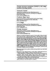
Figure 1: Schematic representation of the B(k) value used to calculate the basin hopping probability of residue k: P(k) = exp(B(k)/RT). The x axis symbolizes a generalized structure coordinate, and the y axis corresponds to the internal free energy surface. -B(k) is a coarse-grained measure of the height of the barrier in the free energy surface that separates the initial and final conformations associated to the basin hopping of residue k. Because the FM algorithm does not try to reproduce dynamicmechanical trajectories, the free energy of the dynamical transition state is not equal in general to F = F0 - B.

630 Colubri et al.

ensures that there is no over estimation of the long-range interactions and no significant bias from the native folds. The selection of torsional coordinates within a basin is a critical element of the algorithm. Its goal is to construct a ϕ-ψ conformation by minimizing the nonbonded energy function using the restrictions of the current set of Ramachandran basins. Ideally, intra-basin sampling should be performed over all residues in every simulation step. There are two obstacles for this approach. It requires extensive amounts of computer time and the current FM energy function is not good enough to generate accurate structures by means of an exhaustive minimization. The latter issue might be regarded as expected, taking into account the coarseness of the model. An optimal packing of spherical side-chains can be quite different from real protein-like structures. In any case, this problem is partially handled by doing exhaustive intra-basin search only on those hopping residues involved in secondary and tertiary structures. This identification of structure is accomplished by using a topological secondary structure detector which is invoked at every step. This detector makes use of the basin information only, and thus it is able to recognize imperfect β-sheet or α-helix structures that lack the regular patterns of backbone hydrogen bonds. This secondary structure assignment is feed into the intrabasin sampler, which then tries to optimize the alignment and connectivity of the secondary elements by minimizing their hydrogen bond energy. The secondary structure assignment is also used to force the coil residues (defined to be those residues not engaged in any regular secondary structure or loop regions) to have hopping probability equal to 1, ensuring that they keep moving until they find a secondary motif that can be optimized. During the intrabasin search, the ϕ-ψ coordinates are selected from the database distribution mentioned above. Using Database Derived Structural Propensities The FM can incorporate structural information from the PDB. This hybrid mode of operation uses database-derived information to include correlations between sequence and secondary structure which are strong enough to bias the basin hopping process. First, it should be noted that any secondary structure prediction or library of fragments can translated to a topological representation in terms of Ramachandran basins. For example, a typical prediction from a secondary structure server can be the string “HHHH EEEEE HHH” where H and E stand for α-helix and β-strand, respectively. Using the naming convention given in the previous section, the former string can be translated as “2222 11111 222”. Thus, the first stage in using any external data-source consists in converting the provided secondary structure information into basin strings that are understood by the FM. Every database-derived method that correlates sequence with secondary structure also has a confidence parameter to measure the reliability of the prediction. This parameter is normalized into a real value V ranging from 0 to 1 used by the FM to decide whether to apply the prediction or not. The hybrid mode in the FM was implemented by replacing step III described before with the following: III´ Determine hopping residues as usual. For each window of length L in the sequence that has a secondary structure prediction assigned to it, calculate the number of non-hopping residues, W, that mismatch the prediction (i.e., their current basin is different from the basin assigned by the prediction). If N/L ≤ V, set the basins to the predicted values for the entire window. If there are overlapping predictions that are accepted simultaneously, use the one with the highest V. If the condition is not meet, and for residues without a secondary structure assignment, select new basins with the default area-based method.

Methodology


Software The FM is a graphical program that can run on Linux or Windows operating systems. The simulations can also be carried out with a command-line version of the FM, called Folding Processor (FP). A 15-node cluster of Linux PCs was used for the computations. As the FP cannot yet run in parallel, a copy of the FP was executed independently on each node. The areas of the Ramachandran basins and the ϕ-ψ intrabasin distributions for each amino acid were calculated with the program RamaEdit (RE), which takes as input a batch of PDB files and then outputs all the Ramachandran maps, allowing also a graphical visualization of the data. The PHD server (21) was used to obtain secondary structure predictions. The requests and subsequent predictions were automatically handled by the program TopSeek (TS), which communicates with the PHD server using its e-mail interface. Simulations Each trajectory simulated with the FP consisted in 100,000 steps. For target T0170 (FF domain of human HYPA/FBP11 protein, 69 residues) 80 simulations were generated. Each simulation for this target took an average of 4 hours on a Pentium III 500Mhz PC. For the other targets, time restrictions limited the calculations to no more than 30 simulations. No all-atom refinement of the final structures was performed, except for a couple of targets in which the side-chains were added and then the steric-clashes were removed by annealing the modified Tinker force-field developed by Freed and Shen (22). The backbone atoms remained fixed during these annealing runs. The simulations were stored in a central server for an automated selection process carried out with the FM. This automated process started by discarding final structures with too high radius of gyration, low contact order (23) or too few number of backbone hydrogen bonds. The remaining structures were sorted according to their energy values. Intermediate conformations were also analyzed to find acceptable structures that were lost by the end of the simulation. Unfortunately, this selection algorithm was in still in development stage at the time and lacked clustering capabilities. Only one or two models were submitted per target. Evaluation of the Results The assessment of the submitted CASP models carried out in the Livermore Prediction Center included a number of different measures that evaluate the global quality of the predicted structures (24). One of these measures is the Global Distance Test Total Score (gdt-ts), which represents an average of the maximum number of residues that can be superimposed between the target and the corresponding model under four different distance thresholds in a standard sequence-dependent manner. The thresholds used are 1, 2, 4 and 8 Å. The formula is the following: Sgdt-ts = (Sgdt-ts(1) + Sgdt-ts(2) + Sgdt-ts(4) + Sgdt-ts(8))/4

[5]

where Sgdt-ts(n) = percentage of residues that can be superimposed under the distance cutoff = n Å. Besides the CASP5 evaluation, an internal comparison between all the generated models and the native structures was performed as well. The aim was to identify in a completely automated manner the best-fit fragments of both submitted and

632 Colubri et al.

non-submitted models, and to look for good models that were not selected. For each model structure, all the fragments between residues n0 and n1 were superposed onto the corresponding region in the native structure and the rmsd for the fragment was calculated. The following score was defined: Srmsd(n0, n1) = crmsd f(rmsd(n0, n1)) + clength g(n)

[6]

where crmsd and clength are coefficients between 0 and 1 such that crmsd + clength = 1, n = n1 – n0 + 1, and the functions f and g are given by: f(r) = r/8 Å if r < 8 Å; ∞ if r ≥ 8 Å

[6a]

g(n) = (N - n)/N if n ≥ 20; ∞ if n < 20 (N = chain length)

[6b]

The best-fit fragment was obtained by minimization of [6] over all possible fragments. The coefficients crmsd and clength allow one to find large fragments close to the native conformation but tolerating some distortions. By minimizing the function f(rmsd(n0, n1)) alone, small fragments with very low rmsd are obtained. By using crmsd = 0.3 and clength = 0.7 however, regions of 60 or more residues with less than 7 Å rmsd are identified. On the other hand, if the overall fold is close to the native structure, any selection of crmsd and clength yield the entire chain. Results and Discussion CASP5 Models Figure 2: Time dependent plots of the best trajectory generated for target T0170. a: Contact order, b: Energy, c: Radius of gyration, d: Rmsd with native structure. All these plots clearly show a sudden collapse in the extent of conformational search at t = 3 × 10-4. At t = 6 × 10-4 and t = 8 × 10-4 to minor conformational rearrangements take place, and after that the simulation reaches the lowest rmsd.

The best FM models were obtained for the α-helical targets T0129 (H.influenzae HI0817 protein) and T0170 (FF domain of human HYPA/FBP11 protein). Both belong to the “New Folds” category, which means their structures did not correspond to any known topology stored in the PDB.


Figure 3: Different snapshots of the best trajectory for target T0170. The native structure is superimposed using with virtual bonds (light gray) and the simulated structure is represented with ribbons (dark grey). a: 0s, b: 1 × 10-4s, c: 4 × 10-4s, d: 5 × 10-4s, e: 6 × 10-4s, f: 7 × 10-4s, g: 9 × 10-4s, h: 1 × 10-3s. It can be appreciated in snapshot h that the N-terminal coil region is not stable and keeps fluctuating, which is the reason for the final increase in the rmsd (see Fig. 2d).

Target T0170 (69 residues) is a 3-helical bundle capped by a 310 helix, which has mild similarity to the C-terminal domain of Phosphatase 2C. The best FM structure has an overall backbone rmsd of 6.22 Å (Fig. 5). The main differences between the model and the native structures are the orientation of the C-terminal helix and the absence of the 310 helix (residues 45-49). Different time-dependent plots and snapshots of the folding trajectory that lead to this structure are shown in Figures 2 and 3. The chain undergoes an intensive conformational search up to t = 4 × 10-4s without forming any persistent interaction. Snapshots of the structures at 0, 1 × 10-4 and 4 × 10-4s, superimposed onto the native structure in virtual bond representation, are given in Figures 3a-c. The t = 1 × 10-4s conformation has a non-native beta-hairpin between residues 19 and 30. A sudden collapse in the structural fluctuations occurs shortly after t = 1 × 10-4s. Interestingly, two of the three native helices have already appeared at that time, but not the N-terminal one. Snapshot 4d (5 × 10-4s) shows that during the collapse, the first helix was formed and the native-like topology was reached, even though the rmsd is slightly below 8 Å. There are two minor rearrangements at t = 6 × 10-4s and t = 8 × 10-4s. Finally, the lowest rmsd is reached at around 9 × 10-4s (Fig. 3g), but comparison with the final structure in Figure 3h (1

Figure 4: Time evolution of the radius of gyration in the trajectory computed for target T0145. Even though there is an early quenching in the structural fluctuations at t = 5 × 10-5, followed by a stable plateau in the radius of gyration, at t = 5 × 10-4 the protein unfolds and remains unstructured during the remaining part of the simulation. This is compatible with the experimental fact that this protein is natively disordered.

634 Colubri et al.

Figure 5: Superimposition of the crystal (red) and best simulated (blue) structures of target T0170. The backbone rmsd is 6.22 Å.

× 10-3s) shows that the reason for the increase in rmsd is basically the fluctuations in the N-terminal coil region. Notice that these small movements drove the rmsd almost to 8 Å, even though the topology remained virtually unchanged. The true structure of target T0129 (182 residues) has two domains (1-90, 91-182). The first domain folds as a distorted up-and-down bundle, while the second domain assembles as a 3-helix left-handed bundle. The best FM generated model matches the experimental structure for the region 12-81 with an rmsd of 6.55 Å (Fig. 6). The separation in two domains was consistently reproduced in all the trajectories, even though the correct structure of the second domain could not be obtained. For other targets with α-helical regions, the models were able to match the experimental structures to within 5 Å rmsd for many fragments varying in length from 30 to 50 residues. For example, fragments for targets T0130 (residues 100-135) and T0135 (residues 25-65) had rmsd of 6 Å and 5.1 Å, respectively (Fig. 7). All these models were generated with the hybrid ab initio/database mode of operation disabled. Unfortunately, the selection algorithm built in the FM was unable to find the best models generated for targets T0170 and T0129. The rmsd of the submitted best fragments is 6.9 Å and 7.23 Å, respectively. Nonetheless, the post-analysis showed that the best models were among the lowest energy structures, even though they were not the energy minimum. The ranking method only included up to the best two models (whereas a total of five were accepted in CASP), so the best models were not submitted. Figure 6: Superimposition of the crystal (red) and best simulated (blue) fragment (12-81) of target T0129. The backbone rmsd is 6.55 Å.

Figure 7: Superimposition of the crystal (red) and best simulated (blue) fragments for other targets than T0129 and T170. a: Fragment (100, 135) of target T0130. The backbone rmsd is 6.0 Å. b: Fragment (25, 65) of target T0135. The backbone rmsd is 5.1 Å.

A summary of the results obtained for all the submitted and best generated models is shown in Table I. The difficulty of each target is strongly correlated with its classification as Comparative Modeling target (CM, “easy”), Fold Recognition target (FR, “medium”) or New Fold target (NF, “difficult”). For the submitted models, the gdt-ts score for the entire structure and rmsd of the best-fit fragment are given. For the best generated model, the rmsd of the corresponding best-fit fragment is shown. As a reference, the gdt-ts score averaged over the best models submitted

for all groups is also given. From the inspection of this table, it is apparent that the FM had an average performance for all the α-helix targets, in terms of the gdt-ts score. The weak performance for the α/β and α+β targets is accentuated by the fact that these were also CM targets with close homologous structures, specially suited for the traditional knowledge-based prediction methods. Natively Unfolded CASP5 Target T0145 Target T0145 (C-terminus of D.melanogaster Gliotactin protein, 216 residues) was removed from CASP5 because it turned out to be a natively unfolded protein. Only one simulation was computed for this target but a close inspection of the trajectory is quite interesting. The evolution of the radius of gyration (Fig. 4) shows that there is no quenching of the structural fluctuations, usually associated with the formation of a stable conformation. There is a drop in the radius of gyration at about 1 x 10-4s, followed by a stable plateau, but it is evident that the protein unfolds at 5 x 10-4s and remains unstructured from that time onwards. Table I Summary of the submitted and best generated models. For each target, the fold category (α, α/β, α+β), the difficulty (CM = Comparative Modelling target = “easy”, FR = Fold Recognition target = “medium” and NF = New Fold target = “difficult”) and the total length of the chain are given in the three first columns. The “Average gdt-ts” column shows the gdt-ts score for each target averaged over the best models submitted by all groups. The gdt-ts for the entire submitted FM model and the rmsd and residues of the best-fit fragment found in the submitted structure are displayed next. Finally, the rmsd and residues of the best-fit fragment extracted from all the generated models is shown. Target

Fold

Difficulty

Length

Average gdt-ts

T0129 - 1 T0129 - 2 T0130 T0137 T0150 T0157 T0170 T0176

α α α/β α+β α/β α/β α α+β

NF NF CM CM CM FR NF CM

89 94 100 133 100 138 69 98

24.66 27.35 32.01 83.83 69.41 39.5 34.64 41.17

gdt-ts 26.12 28.19 20.5 12.22 18.75 17.29 32.61 19.25

Submitted rmsd residues 7.23 32-88 6.68 78-132 7.9 30-80 4.8 1-32 6.85 1-35 2.4 116-136 6.9 15-69 6.6 19-56

Best generated rmsd residues 6.55 12 - 81 3.26 92 - 122 6.5 50 - 108 4.46 19 - 40 5.87 1 - 44 5.47 91 - 123 6.22 1 - 69 6.6 19 - 56

Even though only one trajectory was computed, its behavior is unique. In every other simulation of proteins larger than 100 residues that has been done with the FM, there is always a final quenching in the structural fluctuations. The fact that this protein is natively unstructured is consistent with the unusual behavior observed in the simulated results. This dynamical ab initio result for target T0145 is particularly interesting in view of the predictions of intrinsic disorder on CASP5 targets submitted by Keith Dunker’s group (31). Their approach is completely knowledge based, as they use neural network algorithms trained on long disordered proteins. On one hand, they predicted target T0145 to be entirely disordered and, on the other hand, their prediction for target T0170 was that the entire chain is ordered. These opposite knowledge-based inferences are consistent with the dynamical parameters shown above for both targets. This agreement enforces the idea that a method able to generate not only folded models but also folding pathways, at least in a coarse grained level, might be useful to extract additional structural information, in this case, disorder, that is usually unavailable for the more traditional prediction approaches. Recent Improvements in the Prediction of β-sheet Structures One major problem in the FM algorithm used during the CASP5 computations was its inability to fold complex β-sheet topologies. Before going into the reasons for this weak performance, and the improvements that have been added into the program to solve this issue, it must be point out that, in general, the ab initio genera-


636 Colubri et al.

tion of β-sheet structures is difficult. In other words, all the methods that predict protein structure without using templates obtained by homology tend to perform poorly in structures rich in β-sheets, wherever they correspond to α/β , only β or α+β topologies. In contrast, very good results have been reported in the ab initio prediction of mainly α-helical targets (28). For all the new fold targets in CASP5 that are not fully helical structures, the average Sgdt-ts of the 10 best models from all groups is not greater than 30%, except for the domain 3 of target T0186, which is a small structure (35 residues long) containing 3 β-strands. A detailed summary of the results can be found in (29) and also at the CASP5 website (see Online Resources). These facts help to put in context the results obtained with the FM, and also show that successful ab initio generation of β-sheet structures requires in general improved computational methods. Extensive work has been under progress during the last months to implement a renewed folding algorithm based in the same physical principles of the FM, namely: coarse graining of ϕ-ψ space, kinetically-controlled Monte Carlo transitions and context-dependent energy function. This new algorithm is aimed to extend the range of applicability of the original FM, from small helical structures to complex β-sheet topologies. A full description of this improved algorithm would require an entire article on its own, hence only its main elements will be described here, together with some preliminary results. The improvements can be classified in two broad areas: intra-basin structure optimization and accuracy of the energy function. The original, pattern-based minimization protocol described in Sampling Algorithm was replaced by an unbiased Simulated Annealing algorithm, combined with a gradient-based local minimizer, enabled at the end of each annealing run. The terms of the energy function that were enhanced so far include the steric clashes term, which now is a true LennardJones function, with parameters for the main-chain atoms taken from OPLS AA 2001 (30), and side-chain atoms replaced by a single site together with a radius adjusted to enclose the dimensions of the real side-chain. The explicit main-chain hydrogen-bond energy was also improved, by adding dependency on one more angular parameter and using a better coefficient parametrization obtained by fitting to high-quality PDB data. Test simulations where carried out on proteins with significant amount of native β-sheet structure: protein G (PDB code: 3GB1), de novo designed β-doublet protein (PDB code: 1BTD), and domain 3 of CASP5 target T0183. These simulations are limited in the sense that knowledge of the native structure was used by restricting the energy minimization inside the native Ramachandran basins. The rationale is that at this point the dynamical part of the algorithm is still not under revision, but the more elementary stage of assigning optimal ϕ-ψ coordinates. A preliminary test that should be passed is the ability of finding the native structure in terms of ϕ-ψ coordinates given the native Ramachandran basins. Still, the amount of conformational space that can be explored even after restricting the search inside the native basins is large enough to make these preliminary results very promising. In short, structures below 2.5 Å rmsd were obtained for T0183 and 1BTD (2.33 Å and 1.36 Å, respectively), and the best simulated structure for protein G has an rmsd of 4.20 Å. All these results, and also the new programs used to generate them, both in binary and source-code form, are available at group web page (see Online Resources). Discussion The results obtained so far suggest that is feasible to generate native-like structures by simulating coarse-grained ab initio folding kinetics. In the light of the assessment of the CASP5 models, it is also evident that many improvements both in the sampling algorithm and the parameters of the energy function are needed.

At that point, complex β-topologies cannot be handled, and therefore the FM was limited to α-helix topologies and simple β-sheet structures, such as protein G or ubiquitin. Table I shows the FM was quite unsuccessful in the α/β targets, particularly for target T0137 which has a β-barrel structure. One should appreciate that this target had very high homology to a known structure, hence knowledge-based methods did extremely well. A better intrabasin sampling methodology is required: (a) to accurately locate the turn and hairpin regions, and (b) to generate the correct hydrogen bond pattern that characterizes β-sheet structures. On the other hand, it is encouraging that even with some modules of the FM still under debugging, good results were obtained for some targets. For the “New Fold” targets, the FM generated 2 models within 6 Å rmsd for fragments of about 60-70 residues. It has been demonstrated (25) that the probability of obtaining a model within 6 Å rmsd by a chance is negligible, hence, that a prediction within a 6 Å rmsd should be considered as successful. The case of the unfolded target T0145 indicates that the FM kinetic algorithm might complement the traditional approaches for protein structure prediction which ignore the folding process in the determination of the native fold. The problems with the current energy function are apparent when the generated models were ranked according to their energy values. The assumption that the native structure is the global minimum of the potential was not used. Instead, it was assumed that the native fold is the lowest energy structure among all the kinetically accessible conformations. The following problems were observed: (a) usually the best models were not the energy minima, even though they had low energy values, (b) in certain cases, some incorrect structures appeared to have an energy value substantially lower than most of the generated models, including the best ones. As it was pointed out in the previous section, important improvements in the sampling algorithm and energy function are already being implemented, and the problem of parameterizing energy functions for protein folding is being studied in detail by other groups (26, 27). The preliminary results obtained with the new algorithms are extremely exciting and show that is possible to greatly improve the ab initio simulation of β-sheet structures. All these elements suggest that the approach presented in this article eventually will be much more useful for protein structure prediction. A new article will be prepared as the modules of the more recent simulation programs are finished and debugged. Acknowledgments The author thanks professors A. Fernández, T. R. Sosnick and R. S. Berry for numerous helpful discussions and critical reading of the manuscript, and professor L. R. Scott for providing the computational resources at the Computer Science department. This work was supported by a PMMB postdoctoral fellowship. Online Resources Some of the tools described in this article (RamaEdit, TopSeek and the visualization program used to generate the images of the 3D structures, YAPView), as well the new β-sheet results and the source-code of the latest simulation programs, can be downloaded from: http://sosnick.uchicago.edu/aifoldlab.html CASP5 website: http://predictioncenter.llnl.gov/casp5/Casp5.html PHD server: http://cubic.bioc.columbia.edu/predictprotein/


638 Colubri et al.

References 1. 2. 3. 4. 5. 6. 7. 8. 9. 10. 11. 12. 13. 14. 15. 16. 17. 18. 19. 20. 21. 22. 23. 24. 25. 26. 27. 28.

29.

30. 31.

C. Soto. Nature Neuroscience 4, 49-60 (2003). P. Romero, Z. Obradovic, X. Li, E. Gardner, C. J. Brown, K. Dunker. Proteins 42, 38-48 (2001). A. Fernández, A. Colubri, R. S. Berry. PNAS 97, 14062-14066 (2000) K. Kuwata, R. Shastry, H. Cheng, M. Hoshino, C. A. Batt, Y. Goto, H. Roder. Nature Str. Biol. 2, 151-155 (2001) Y. Duan, P. A. Kollman. Science 282, 740-744 (1998) A. Fernández, T. R. Sosnick, A. Colubri. J. Mol. Biol. 321, 659-675 (2002) H. Hu, M. Elstner, J. Hermans. Proteins 50, 451-463 (2003) M. H. Zaman, M. Y. Shen, R. S. Berry, K. F. Freed, T. R. Sosnick. J. Mol. Biol. Submitted. C. D. Snow, H. Nguyen, V. S. Pande, M. Gruebele. Nature 402, 102-106 (2002) D. Fischer, D. Rice, J. U. Bowie, D. Eisenberg. FASEB Journal 10, 126-136 (1996) M. S. Johnson, J. P. Verington, T. L. Blundell. J. Mol. Biol. 231, 735-752 (1993) R. Bonneau, J. Tsai, I. Ruczinski, D. Chivian, C. Rohl, C. E. Strauss, D. Baker. Proteins 45 Sup. 5, 119-26 (2001) A. R. Fersht, A. Matouschek, L. Serrano. J. Mol. Biol. 224, 771-782 (1992) A. Fernández, A. Colubri, R. S. Berry. Physica A 307, 235-259 (2002) A. Fernández, A. Colubri, R. S. Berry. J. Chem. Phys. 114, 5871-5887 (2001) A. Fernández, A. Colubri. Proteins 48, 293-310 (2002) A. Colubri, A. Fernández. J. Biomol. Str. & Dyn. 19, 739-764 (2002) A. Fernández. J. Chem. Phys. 115, 7293-7297 (2001) M. B. Swindells, M. W. MacArthur, J. M. Thornton. Nature Str. Biol. 2, 596-603 (1995) D. Walther, F. E. Cohen. Acta Cryst. D 55, 506-517 (1999) B. Rost, C. Sander. J. Mol. Biol. 232, 584-599 (1993) K. F. Freed, M. Y. Shen. Proteins 49, 439-445 (2002) R. Bonneau, I. Ruczinski, J. Tsai, D. Baker. Protein Science 11, 1937-44 (2002) A. Zemla, C. Venclovas, J. Moult, K. Fidelis. Proteins 37 Sup. 3, 22-29 (1999) B. A. Reva, A. V. Finkelstein, J. Skolnick. Fold. Des. 3, 141-147 (1998) J. Lee, D. R. Ripoll, C. Czaplewski, J. Pillardy, W. J. Wedemeyer, H. A. Scheraga. J. Phys. Chem. B 105, 7291-7298 (2001) T. Lazaridis, M. Karplus. J. Mol. Biol. 228, 447-487 (1998) P. Bradley, D. Chivian, J. Meiler, K. M. S. Misura, C. A. Rohl, W. R. Schief, W. J. Wedemeyer, O. Schueler-Furman, P. Murphy, J. Schonbrun, C. E. M. Strauss, D. Baker. Proteins 53 Sup. 6, 457-468 (2003) Proceedings of the Fifth Meeting on the Critical Assessment of Techniques for Protein Structure Prediction. Asilomar Conference Center, Pacific Grove, California. December 1-5, 2002 G. Kaminski, R. A. Friesner, J. Tirado-Rives, W. L. Jorgensen. J. Phys. Chem. B 105, 64746487 (2001) Z. Obradovic, K. Peng, S. Vucetic, P. Radivojac, C. J. Brown, A. K. Dunker. Proteins 53 Sup. 6, 566-572 (2003).

Date Received: May 19, 2003

Communicated by the Editor Ramaswamy H Sarma